 A. Picallo-Perez1*
 J. M. Sala-Lizarraga1C. Escudero-Revilla1
 J. M. Hidalgo-Betanzos1,2I. Ruiz de Vergara2
- 1Research Group ENEDI, Department of Thermal Engineering, University of the Basque Country (UPV/EHU), Bilbao, Spain
- 2Thermal Area of the Laboratory of Quality Control of Buildings of the Basque Government, Vitoria-Gasteiz, Spain
In this work thermoeconomics is applied to a central thermal system covering three buildings that consists of a cogeneration engine, an aerothermal heat pump and a natural gas condensing boiler. Cogeneration systems integrated with renewable energy technologies are very attractive solutions in the building sector. Nevertheless, the use of cogeneration systems together with active envelope solutions, such as the one encountered in this work, are scarce and the efforts to enhance the synergies between both systems are even scarcer. A heat pump is connected to a so-called solar wall to provide hot air and a renewable photovoltaic system supplies the electricity consumed by the heat pump. Thermoeconomics is applied to evaluate the cost of flows based on its energy-quality. Hence, this innovative and complex system can be analysed and diagnosed by this methodology. As a result, thermoeconomics is presented as an effective tool for the detailed study of the energy cost distribution and the key to enhancing energy efficiency.
1 Introduction
Due to the high-energy consumption and GHG emissions of the building sector, buildings are responsible for almost 40% of the global energy consumption (Li et al., 2021) and many efforts are being made to decrease the energy demand and increase the efficiency of thermal systems, without affecting the Indoor Environment Quality (IEQ) (Korsavi et al., 2020). Demand needs to decrease in order to achieve the environmental objectives set by the European Commission (Verhaeghe, 2020). Innovative actions, both in the thermal envelope and through the implementation of renewable technologies, make it possible to reduce energy consumption while also enhancing the interior comfort of buildings to improve the quality of life. Moreover, the current context is characterized by exceptional conditions in which the economic crisis, accelerated by the current COVID-19 health crisis, converges with the need to increase the IEQ of buildings.
Traditionally, buildings have produced the required thermal demand by means of combustion equipment, such as boilers. Nowadays, technologies that are more sophisticated are being pursued to adapt more efficiently to the thermal levels of demand; such as sustainable solutions that comprise heat pumps, solar thermal systems or even hydrogen based cogeneration systems (Cheekatamarla et al., 2021). After all, buildings require heating and cooling, at a temperature a few degrees above or below the ambient temperature, domestic hot water (DHW) at around 60°C, or electricity, which is a high-quality energy. The use of waste heat, or of some renewable sources, makes it possible to cover low-quality demands by adapting more efficiently to thermal levels. Combustion or electric equipment can be used to cover high-quality demands, such as household appliances or lighting. The result of adapting the technologies to specific uses can help to create more energy efficient buildings and decrease the environmental issues.
Due to their energy and environmental advantages, polygeneration systems combined with renewable energy technologies (also known as hybrid polygeneration systems) are now being examined in many works of research. A review to outline the latest developments on integrated polygeneration and renewable systems, for desalination, is done in Khoshgoftar Manesh and Onishi. (2021); a polygeneration hybrid solar and biomass system is investigated in Sahoo et al. (2018); solar-driven polygeneration systems are summarized and discussed in Ref. Kasaeian et al. (2020). The optimal design and the performance analysis of solar hybrid polygeneration system is analysed in Yang and Zhai. (2019) by considering different building types and climate conditions, and in Yang and Zhai. (2018) considering different operation strategies. In fact, the combination of these two technologies, polygeneration and renewable energies, provides several advantages: 1) primary energy conversion efficiency is higher compared to traditional systems, and 2) renewable energy-based technologies have less impact on the environment.
However, hybrid polygeneration systems have seldom been used in building systems because there is a necessity to investigate the integration of the said technologies as well as the optimal energy management. The influence of legal constraints on the integration of renewable energy technologies in polygeneration systems for buildings was analysed in Pina et al. (2021). In the case of cogeneration, also known as Combined Heat and Power (CHP), this has a much lower economic return on buildings than on industry. This is because:
• The demand is very variable, as it depends on climatic factors and on the behaviour of the users, which is difficult to predict;
• As the power of the facilities in buildings is lower than in industry, economies of scale come into play.
However, technologies for small-power cogeneration and micro-cogeneration or polygeneration systems can provide the energy services demanded in buildings (electricity, DHW, heating and cooling), all with high-energy efficiencies, and with the consequent economic benefit and lower environmental impact. The technical and economic viability of micro-cogeneration systems in buildings is discussed in Atănăsoae. (2020) while Cheekatamarla et al. (2021) search sustainable solutions in buildings by analysing cogeneration systems. Furthermore, new analysis strategies have arisen in the last few decades enabling us to better understand energy use and its degradation, as is the case of thermoeconomics (TE).
1.1 Thermoeconomics in Building Thermal Systems
Thermoeconomics (TE), based on the first and second laws of thermodynamics, aims to promote energy savings and sets the guidelines for a better energy use; a fact that also decreases the environmental impact, making the service sector a sustainable sector for its application. TE is a relatively young science, developed for the industrial world, which is rarely applied in the building sector. Different thermoeconomic methodologies are explained and compared in Picallo-Perez et al. (2021a). Consequently TE aims to detect the points of highest irreversibilities and losses (and therefore costs) in order to obtain a rational picture of the cost formation process. This information is very useful when implementing improvement and control optimization actions with the aim of reducing costs and promoting energy savings, which cannot be obtained with classical analyses based on energy conservation.
Therefore, TE relates Physics with Economics through the concept of exergy cost, since exergy is an appropriate thermodynamic property, as it takes into account the quantity of energy and its quality, understanding by quality its capacity to do something useful (de Renobales, 1995). Thermoeconomics makes it possible to solve problems that cannot be solved with traditional energy analyses based on the first law, such as:
• Determining the costs of the products of a facility based on physical criteria, see an example in Valero et al. (2006).
• Detecting the places where losses actually occur, evaluating their costs and proposing cost-effective improvements.
• Diagnosing facilities, see the tool developed in Picallo-Perez et al. (2021b).
• Optimizing decision variables in the design of equipment and facilities, Piacentino and Cardona. (2007).
The applications of TE in the industrial field date back to the end of the last century. However, applications in non-industrial areas started to be explored in the 2010s, as for example in Picallo-Perez et al. (2017a) and Picallo-Perez et al. (2017b); a detailed literature review appears in Abusoglu and Kanoglu.( 2009) and Keshavarzian et al. (2018). As far as the building sector is concerned, these works are scarcer. The book of Sala and Picallo. (2020) was published in 2019 and it comprehensively analyses buildings; both the envelope and facilities, from an exergy point of view, applying thermoeconomics for design, optimization and maintenance purposes1.
Even if scarce, some works can be found in the literature concerning TE application in hybrid polygeneration systems. In Yang et al. (2018), for example, a TE analysis is done for calculating the exergetic cost of a combined cooling, heating and power system of a hypothetic hotel, highlighting that exergetic cost is seldom assessed in this type of systems. In Mouaky and Rachek. (2020) a solar and biomass hybrid polygeneration system is analysed under the thermodynamic and TE point of view using a model developed by Ebsilon Professional software. A polygeneration system supplied by solar, geothermal and biomass resources is optimized and deeply analysed in Calise et al. (2021). However, the TE analysis done is based only in some economic parameters and not in exergy costs. Conversely, exergy costs are accounted in Martínez-Gracia et al. (2021) where also a complementary method is offered to assess and better understand the efficiency of a cogeneration solar configuration. Therefore, even if some works exist, the methodology to apply TE in building polygeneration systems (based on exergy costs) should be enhanced. After all, productive structure definition can be sometimes tedious or difficult. This work, besides applying TE based on exergy costs approach, proposes a simplified methodology to define the productive structure of the system and defines new indexes based on exergy terms to analyse CHP systems.
1.2 Objectives and Overall Organization
In this work, the central thermal polygeneration system of a set of three buildings is analysed. It consists of a cogeneration engine, a natural gas condensing boiler and an aerothermal heat pump provided with renewable PV electricity and working in connection to a solar wall. These buildings are social housing blocks, where heating and DHW cost minimization is one of the main goals.
In Section 2, after analysing the advantages of including cogeneration through the calculation of its respective indices, the basis of a general thermoeconomic model is set out. In Section 3 the above developments are applied to the set of three buildings of our case; thermoeconomics is applied to check and detect the most unfavourable thermal processes and control strategies in terms of energy costs. In Section 4, the numerical results obtained are shown and analysed. At the end of this Section, a discussion of the results obtained and some conclusions are set out and the savings coming from renewable energy use are quantified.
2 Materials and Methods
This section contains brief mathematical formulae to follow the case study and the numerical results finally obtained.
2.1 Cogeneration Energy and Exergy Indexes
Cogeneration sequentially produces electricity (E) and useful heat (H) from the same fuel (F), having an energy efficiency defined as:
In order to incorporate it in building systems, the promoter must decide whether to install it or to proceed in a conventional manner, by buying electricity from the grid (produced with
The Percentage of energy saving (PES) is
In the case of installations of less than 1 MWe, which is the most common case in buildings, the PES needs to be positive to be considered as a high efficiency system (Official Journal of the European Union, 2004).
The equivalent electrical efficiency (
This index allows the electrical efficiency of a CHP plant to be compared with the electrical efficiency of a plant that only produces electricity.
In parallel with these indices, similar indices can be defined in terms of exergy. For that, the exergy efficiency of a cogeneration plant is defined as the relationship between the electricity (E) plus the thermal exergy produced (
This efficiency considers the real losses or irreversibilities in the cogeneration process. Its value is lower than the energy efficiency, since it considers the quality of the energy and not only the quantity. Indeed, even if electricity is all exergy, the thermal energy produced is low-quality energy, so its exergy content is much lower than its energy, whereas the fuel used has a quality factor near one.
The Exergy Saving (ExS) is defined in an analogous way:
where
Similarly, the Equivalent Electrical Exergy Efficiency (
2.2 Thermoeconomic Model
As the name suggests, thermoeconomics combines economic models with physical energy models to, among other things, calculate the costs (exergetic and economic) of the flows along a system.1 The term cost refers to the amount of resources required to obtain the specific ith flow, (
• Proposition 1: The exergy cost is conserved, so
• Proposition 2: If there is no extra evaluation, the external incoming exergy unit cost of resources is equal to one
• Proposition 3: All costs generated in the process are assigned to the final products. Therefore, losses have null costs.
• Proposition 4: It is divided into two parts: (4.1) if the jth flow is an outgoing flow of a subsystem and belongs to the incoming ith flow of that subsystem, both flows have the same unit cost,
TE also uses the productive model of the system. The productive model refers to the interactions between components in terms of Fuels (F) and Products (P): F considers the amount of resources needed in the process, and P reflects the purpose of the process. Therefore, the cost can be given in terms of the costs of fuel and the product of an ith component (
Accordingly, all the propositions can be introduced in a common matrix formula that contemplates the whole system; so the fuels and products of all the components are represented by its vectors (
Likewise, the vectors of the unit exergy costs of fuels and products (
These unit exergetic costs give the information of the cost distribution along the system.
Accordingly, on the one hand, the unit cost of fuel of an ith component
On the other hand, the difference between the unit cost of the product and fuel of an ith component
The total exergy costs of the fuels and products are simply achieved by multiplying the unit costs by their exergy.
2.1.1 Influence on the Cost of Renewable Energies
As already said, the exergy costs reflect the degradation of energy along a system, pointing out the places with higher irreversibilities by means of higher costs. These costs refer to the amount of resources (in kWhex) needed to provide a certain flow, therefore, it only considers the fuel consumption without taking into account the cost related to the acquisition, operation and maintenance costs. However, expressing the fuel consumption costs in economic units (in €) can be more attractive for a cost analysis. Indeed, this is the way to emphasize the advantage of using renewable energies.
Hence, we define the unit exergoeconomic costs of each external resource as the cost per unit of exergy (
On the other side, when total costs are taken into account, zp vector needs to be considered whose elements contain the costs of acquisition, operation and maintenance per unit of products2.
2.1.2 Flow Chart of the Methodology
Therefore, the methodology to be followed is summarized in Figure 1. Accordingly, this work is devoted to calculate the following values:
• Cogeneration Energy indexes
• Cogeneration Exergy indexes
• Exergy costs of components
• Exergoeconomic costs of system components
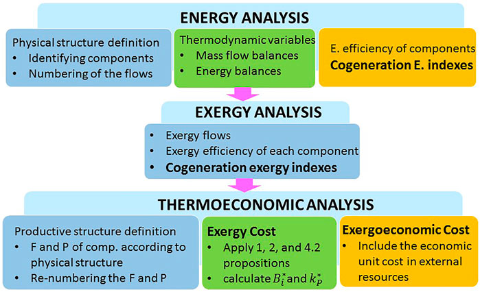
FIGURE 1. Flow chart of the methodology.
3 Case Study
3.1 Description of the Buildings
The set of buildings are in Portugalete (the Basque Country, in northern Spain), on a plot of land with a 10% of slope. There are three adjacent five-floor buildings, with two dwellings per floor. There are also two underfloor parking spaces, Figure 2.
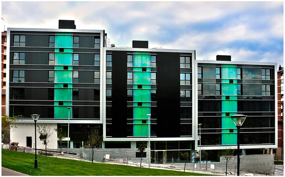
FIGURE 2. Photograph of the three buildings.
These buildings are part of the Basque Government’s social housing, where homes are provided to low-income people for 5 years with a low rent; because of that these buildings are design to have a very-low energy demand for heating.
The main problem is that most of the users could be unable to pay the community charges, so the buildings are designed to reduce energy consumption to a minimum. In order to avoid such a state of affairs, these buildings have some particularities, incorporating passive systems, renewable energies and cogeneration.
Related to the architecture of the buildings, the façades facing the North, West and East are conventional, with the following thermal transmittances:
• 0.26 W/m2K for opaque elements (composed of a sandwich panel, polyurethane, rock wool, cellular concrete and plasterboard).
• 2.2 W/m2K for windows (low emissivity glass 6/12/4).
• 0.3 W/m2K for the roof (extruded polystyrene).
The South façades of two of these buildings, conversely, have two different types of active façade solutions3:
• One is a Trombe wall connected to the ventilation system through a heat recovery system.
• The other is a solar wall connected to the heating system, providing hot air to a heat pump placed on the roof.
Furthermore, there are 88 PV panels (with 22.4 kW of installed power) placed on the roof to feed the heat pump and the lifts.
3.2 Thermal Facility
The thermal installation consists of radiant floor heating and DHW distribution for 32 dwellings in three blocks. Heat is generated in three main elements: a cogeneration engine, an aerothermal heat pump and a natural gas condensing boiler.
• The 12.5 kW thermal power and 5.5 kWe electric power cogeneration engine serves a so-called high-temperature branch, and for energy efficiency reasons, it is in operation for as long as possible.
• The 12.9 kW rated power heat pump serves a so-called low temperature branch and has the second priority after the micro-cogeneration equipment, especially when there is no heating demand.4
• The 102 kW nominal power condensing boiler supports the previous engines and works with a lower priority, when the micro-cogeneration equipment and the heat pump are not able to cover the heating and DHW demands of the buildings.
There is also auxiliary equipment to transfer thermal energy and to provide the necessary inertia for the heating and the DHW of each dwelling, such as heat exchangers, 2000 L tanks and valves. Figure 3 groups the main equipment and shows the scheme of the installation.
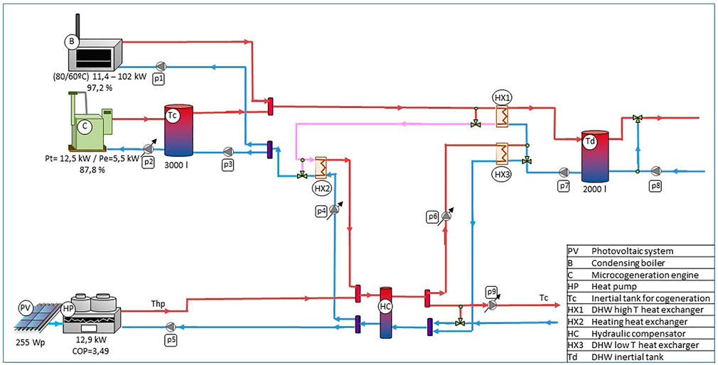
FIGURE 3. Main equipment summary and scheme of the installation.
3.1.1 Thermal Facility Control
As said, one of the main limitation to the CHP diffusion in residential buildings is due to the high variability of the demand, which depends on the climatic factors and on the users behaviours. For such a reason the adopted control logic plays a crucial role. The control is divided into two main sets: the DHW circuit control and the heating circuit control; the system control logic flowchart is in Figure 4.
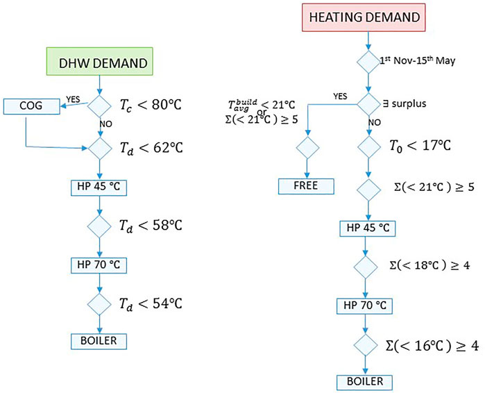
FIGURE 4. System control logic flowchart.
In the case of the DHW demand, the priority order of the stages is as follows:
• First, the cogeneration engine turns on to keep the DHW tank at 80°C.
• Then, the heat pump starts in low temperature mode, at 45°C.
• Subsequently, if the DHW demand cannot be covered, the heat pump changes to high temperature mode, at 70°C.
• Finally, if necessary, the boiler is turned on.
Heating demand is turned on according to a yearly schedule (from November 1st to May 15th), as well as to the outside temperature. The heating operates if the outside temperature is below 17°C and there is a minimum number of dwellings (at least 5) demanding heating through their individual thermostat, until 21°C is reached.
The heat pump provides mainly heating, as the terminal elements correspond to a radiant floor. If the heating is running and the heat pump cannot handle the demand, the heat pump starts working at the high temperature level by proportionally regulating the valve of the third heat exchanger (HX3) so that the micro CHP and/or the boiler can support it.
If, above all, there is sufficient surplus in the electrical power (coming from the PV cells and CHP engines), the heat pump will be activated. That will happen if:
• The average ambient temperature of the building is below 21°C.
• A minimum number of dwellings (5) have their ambient temperature below 21°C.
If one of these two cases occurs, the radiant floor heating will be started “free of charge” to all dwellings below 21°C to heat the building in general terms. In the event that the building’s average temperature rises above the setpoint, or the surplus for the “free” mode is terminated, free-heating will be stopped.
3.3 Thermoeconomic Model
All the equipment and its control has been modelled in Trnsys Studio (Trnsys, 2000) interface by including the corresponding nominal characteristics to each Type/component. These are the corresponding Types for the energy generation:
• Boiler: Type 70
• CPH: Type 154
• Heat pump: Type 941
• PV panels: Type 562e
The corresponding demands are included through an external document read by a Data-reader Type 9a. Such demands are obtained directly from the building’s monitoring system, where the DHW Li et al, 2021 demand and the heating demand (kWh) are extracted every minute. The environmental temperature is also monitored, so real temperatures are used for the system control. The radiation meteorological data was taken from the Meteonorm database (Remund, 2008). The simulation was done for the heating period with a time step of 15 min.
The physical model of the system envisages the 54 flows and components used for the thermoeconomic analysis, Figure 5.
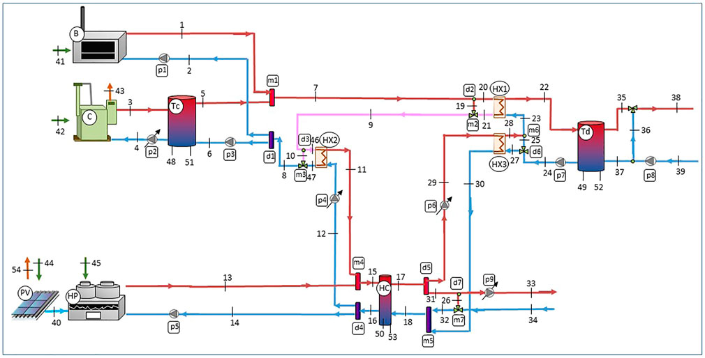
FIGURE 5. Physical model of the system with numbered flows and components.
The productive model, on the other hand, reflects the interactions between components in terms of Fuels and Products. It is worth highlighting the fact that the approach followed was the one of a productive super-structure explained in Picallo-Perez et al. (2019). In this way, the dynamism of the system was accounted for by means of productive specific-structures that adapt, at each time-step, to the modulating operating conditions; that is, only the active components and flows are considered for the specific productive structure at that time, which is created by erasing the non-active components and the non-active flows from the productive super-structure.
Likewise, the productive structure of the inertial components were defined according to the method developed in Picallo-Perez et al. (2020); i.e., the Tc, HC, Td. Accordingly, two virtual flows are included for each component, referring to the charging and discharging periods: (
The productive super-structure is depicted in Figure 6 according to the flow numbering of Figure 5. Fuels are defined as the entering arrows and products as the outgoing arrows. Real components are identified with 10 squares, junctions with 19 circumferences and bifurcations with 19 diamonds. So there are 48 components, some are real and others virtual.
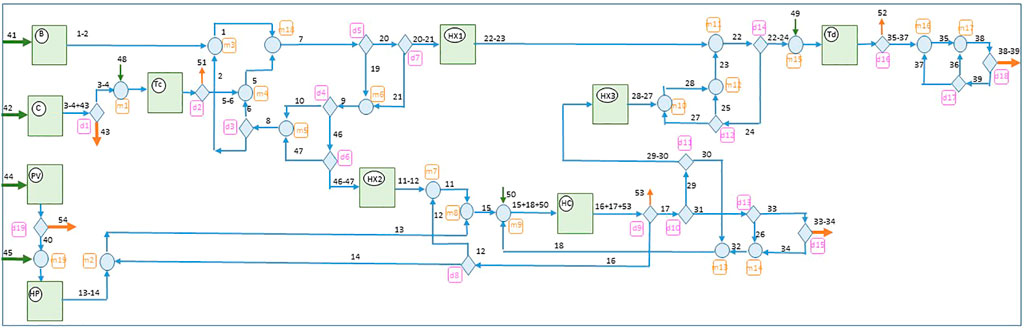
FIGURE 6. Productive Super-structure of the thermal system according to the flows numbering of Figure 5.
3.3.1 A Simplified Method for Applying Thermoeconomic Propositions
Applying TE propositions in the productive super-structure of Figure 6 seems to be tedious and non-intuitive due to the great amount of components. However, if each arrow is related to only one number/flow, the method becomes direct and easy to apply. This section shows a direct way to apply TE propositions methodologically.
To do so, each component, either real or virtual, needs to be defined with only one entering flow-number and one outgoing flow-number. The said flow-number considers the global “cumulative flow”, i.e., it is the sum (or subtraction) of the physical flows specified in the productive super-structure of Figure 6. Accordingly, the productive super-structure is re-named in Figure 7. As a result, there are now 48 components and 75 flows.
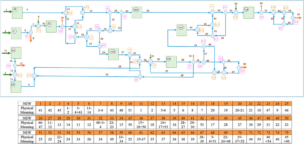
FIGURE 7. : New Numbering and definitions of flows in the Productive super-structure to facilitate the application of proposition.
As the aim of thermoeconomics is to account for the exergy cost distribution along the system, i.e., to calculate the costs of 75 flows, there are 75 unknown values. So we need a system of 75 equations to calculate each exergy cost. Nevertheless, defining propositions in this re-named super-structure is much easier and direct; indeed, only three propositions are needed:
• Proposition 1: All the fuel costs are equal to all the product costs in each component; therefore, as there are 48 components, we have 48 equations as:
• Proposition 2: All the external resources have a unit exergy cost equal to one. As there are 7 entering resources, they follow 7 equations:
• Proposition 4.2: One equation at least can be defined for each bifurcation. As there are 19 diamonds and one has 3 products, there are 20 equations.
Consequently, we obtain a system of 48 + 7+20 = 75 equations to apply the corresponding matrix formulae. The F and P of all the components, as well as the propositions, are shown in Table 1, except for the proposition
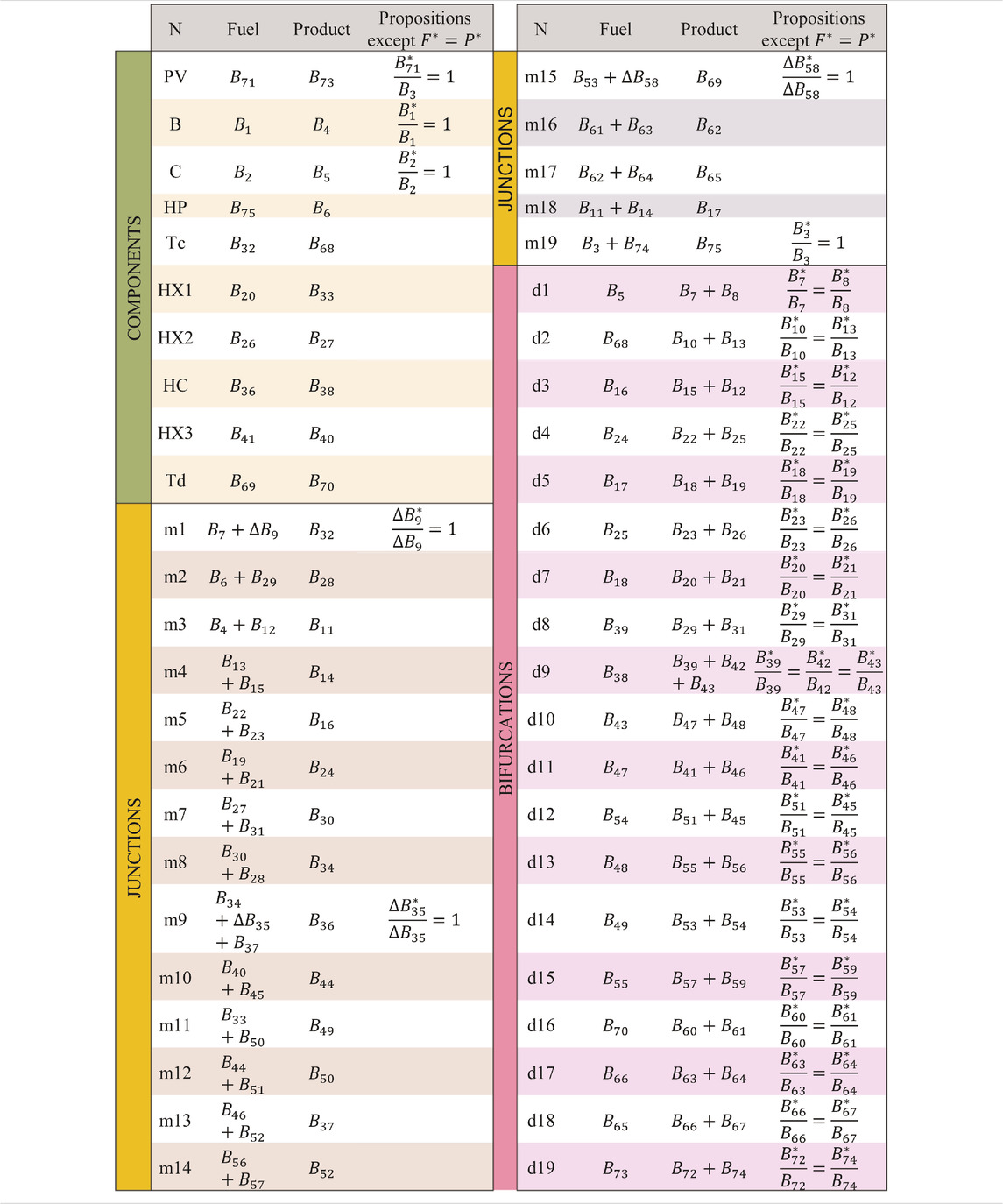
TABLE 1. Main definition for thermoeconomic matrix formulae.
4 Numerical Results
This section briefly contains the main results related to the thermoeconomic application to the cogeneration system.
4.1 Energy Performance
The facility was modelled in Trnsys and simulated during the heating period, with a 15 min time-step and the control explained above. As the simulation model and the energy analysis are beyond the scope of this work, only the results referring to the generator engines and the demands and production are shown.
Figure 8 depicts the dynamic behaviour fuel consumption of the engines and the external climate conditions during the third week of March. As can be seen:
• Cogeneration (C) is on all the time thanks to the inertial tank (Tc) associated with it. The heat pump (HP) and the boiler (B) enter subsequently, when the temperature of the DHW tank is below the defined setpoint (this tank (Td) gives inertia to the system so that the activating moments of HP and B occur after a temperature drop).
• The solar radiation is variable due to its dependence on the hour of the day and the climatic conditions.
• The average energy and exergy efficiency of the generator components in the heating period are in Table 2. Even if the HP has a COP higher than 1, its exergy efficiency is very low because it transforms electricity into low temperature heat. Something similar happens with B and C, which produce heat from combustion; however, as C also produces electricity, its exergy efficiency is higher. The energy and exergy efficiencies of the PVs are similar, as the exergy of the solar radiation is similar to the energy.
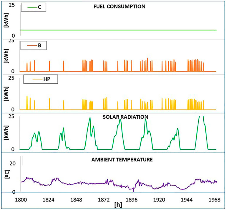
FIGURE 8. Fuel consumption along a week in March.
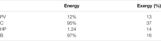
TABLE 2. Energy and exergy efficiency of generator engines.
Figure 9 shows the heating and DHW demands, as well as the electricity generation of CHP and the electricity surplus of the PV cells. As can be seen:
• DHW demand is almost “periodic” along the week, while the heating demand is very variable, depending on the user profiles and ambient conditions.
• Electricity production in C is constant because it depends on the cogeneration engine, while the electricity surplus in the PV panels depends on the solar radiation (this electricity is the subtraction between the PV production and the HP consumption, when positive).
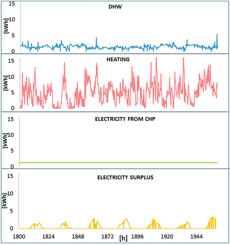
FIGURE 9. Demand and electricity production along a week in March.
4.2 Cogeneration Energy and Exergy Indices
The accumulated values along the heating season were used to calculate the cogeneration indices, Table 3.
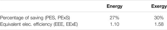
TABLE 3. Cogeneration indices in energy and exergy terms.
The Percentage of Energy Saving (PES) and Percentage of Exergy Saving (PExS) were calculated with the following efficiencies, taken from Spanish Government. (2016):
According to the results obtained, the following is observed.
• Even in energy or exergy terms, cogeneration is preferable to separate production (since the PES and PExS indices are positive). Moreover, the percentage in savings is more marked in exergy terms. This is because generating heat separately requires more exergy consumption due to the low exergy efficiency of the boiler.
• The same happens with the EEE and EExE indices, which both reflect the suitability of cogeneration.
4.3 Thermoeconomic Analysis
The TE analysis distributes the unit exergy cost throughout the system according to the fuel (F) and product (P) definitions of each component. As the results for real components are the interesting ones, Table 4A gathers the values of the F, P, irreversibility (I) and the unit cost of fuels (
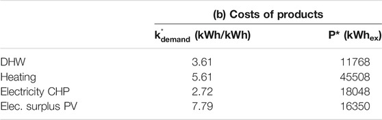
TABLE 4A. Thermoeconomic results (a) of real components (b) of products.
The results can be summarized as follows:
• The
• The heat pump (HP), however, consumes part of the electricity coming from PV and part from the net (when there is not enough PV generation); therefore, its
• C generates the highest irreversibilities of the system. This is because I is an extensive property and gets bigger as more fuel is consumed. To be precise, C is activated as much time as possible in order to profit from the electricity cogenerated.
• However, the unit exergy consumption increment (i.e., the
• The HP is less efficient than B since its
• Even if this system cannot be considered sequential at all, as the components are placed downstream, their
The most interesting values are the exergy costs of the outgoing products
Accordingly, in unit exergy terms, heating is more expensive than DHW. In relation to electricity generation, the electricity from cogeneration requires fewer resources than the electricity coming from renewable solar radiation. Therefore, a priori, the CHP system seems to be a better alternative than PV cells, due to their lower exergy efficiency.
4.3.1 Influence on Cost of Renewable Energies
As said above, the exergoeconomic analysis expresses the costs in monetary units. The cost per unit of exergy for each external resource is, in our case:
•
•
• and,
Table 5 summarizes the results of the exergoeconomic analysis in two cases: 1) when all the electricity comes from the grid without considering the PV renewable production, and, 2) including the PV production. These results are only related to the external resource consumption, without considering the acquisition, operation and maintenance costs of each component. Therefore:
• As
• Only the components associated to the HP branch have different costs:
HX3: decreasing from
Td: decreasing from
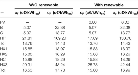
TABLE 5. Exergoeconomic results without and with renewable electricity.
The unit exergoeconomic costs and the total cost of the final products (DHW, heating and electricity) are shown in Table 6. As said, these costs do not consider the acquisition, operation and maintenance costs of the components, but show the benefits of combining renewable sources with polygeneration systems; a result that was misinterpreted in the previous exergetic analysis.
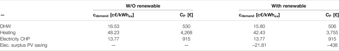
TABLE 6. Exergoeconomic unit and total costs for products.
The electricity consumption in this table is divided into two parts:
• Electricity obtained from the CHP.
• Electricity obtained from the PV surplus, which instead of selling to the grid covers some community consumptions (lifts and illumination).
Therefore, the PV panels’ surplus substitutes the grid consumption, so it can be though that
In consequence, there are two main savings due to the renewable energy incorporation:
• The savings due to the costs reduction in DHW and heating equal to 537 €/year.
DHW: unit cost decreasing from
Heating: unit cost decreasing from
• The savings obtained due to the electricity surplus consumed in lifts and illumination which substitutes the purchase from the grid at
So, the net saving due to PV panels is equal to 975 €/year.
5 Conclusion
This work analyses a central thermal system of three buildings consisting of a CHP cogeneration engine, an aerothermal heat pump (supplied by PV electricity) and a natural gas condensing boiler.
• PES is positive (27%).
• Exergy values reflect better the advantage of producing electricity in a combined way (EExE = 1.58) than in energy terms (EEE = 1.1).
Consequently, exergy is a very useful property to locate the real losses and the profitability of transforming energy from one type to another. In this way, such combustion equipment as boilers or CHP systems, are heavily penalized under the exergy point of view, because they transform a high-valuable energy flow of fuel to a low-quality heat flow, resulting in:
• Exergy efficiency of the cogeneration engines is
• Exergy efficiency of the boiler is
• Exergy efficiency of HP is
• Exergy efficiency of renewable technologies, such as photovoltaic panels, is
These are the results according to the thermoeconomic analysis:
• The DHW unit exergy cost is 3.61 (kWh/kWh).
• The heating unit exergy cost is 5.61 (kWh/kWh).
• In addition, cogenerating electricity is cheaper [2.72 (kWh/kWh)] than generating it from PV panels [7.79 (kWh/kWh)] because of the irreversibilities encountered in the conversion of solar radiation and electricity.
However, the exergoeconomic costs highlight the benefits of using renewable energy; these costs are only related to the fuel consumption costs without considering the acquisition, operation and maintenance costs. As the cost of solar radiation is null,
• The yearly saving, due to exergoeconomic unit cost reduction in DHW and heating, thanks to PV renewable panels, is 537€/year.
• And the savings obtained due to the electricity surplus in PV panels is equal to 438 €/year.
6 Discussion
The potential for introducing CHP systems in the building sector is very high, but practically unexploited. In relation to industry, the main disadvantage of introducing cogeneration in buildings is that the thermal demand is very variable and the power of the equipment needed is smaller. Nevertheless, the dynamism of thermal demand can be avoided somewhat by using thermal inertial systems to cover the decoupling between production and demand. In addition, in order to ensure the constant functioning of the CHP systems, they are usually undersized and auxiliary generation systems, such as heat pump and boilers, are included to help in peak demand periods.
On the other hand, the costs occasioned by the irreversibilities along the systems can be accounted for by thermoeconomics (TE). TE makes a rational distribution of costs, i.e., it accounts for the amount of resources required to achieve a specific objective, on an exergy base. Along this work, an easy-to-apply method has been explained to apply TE propositions in a system with a high number of components. This method is dynamic and can be applied successively, no matter how many components or flows there are.
Nevertheless, to evaluate the total cost, we must take into account the acquisition cost and the operation and maintenance costs. In the same way, when evaluating the income from the sale of cogenerated and PV electricity, the complement for efficiency, the complement for reactive energy, the costs of deviations, etc., as well as the maintenance costs for the whole components of the system, must be taken into account. Likewise, the insurance and financing costs must also be considered.
Furthermore, renewable technology can be related to the environmental impact generated along its useful life (from cradle to grave). Accordingly, the exergoenviromental analysis considers the environmental impact associated with the generation of the flows. It is an approach analogous to exergetic and exergoeconomic analyses and uses Life Cycle Analysis (LCA) to calculate the unit exergoenvironmental costs of the fuels and products (
Data Availability Statement
The datasets presented in this article are not readily available because they are ENEDI research group data. Requests to access the datasets should be directed to YW5hLnBpY2FsbG9AZWh1LmV1cw==.
Author Contributions
AP-P: Writing-Original draft preparation, Data curation, Conceptualization, Formal analysis, Methodology, Software, Validation/JS-L: Writing- Reviewing and Editing, Conceptualization, Methodology, Formal analysis, Visualization, Investigation, Supervision/CE-R: Investigation, Reviewing and Editing./JH-B: Software, Validation/IR: Original draft preparation, Reviewing and Editing.
Funding
This work has been partially funded by the Land Planning, Housing and Transports Department of the Basque Government.
Conflict of Interest
The authors declare that the research was conducted in the absence of any commercial or financial relationships that could be construed as a potential conflict of interest.
Publisher’s Note
All claims expressed in this article are solely those of the authors and do not necessarily represent those of their affiliated organizations, or those of the publisher, the editors and the reviewers. Any product that may be evaluated in this article, or claim that may be made by its manufacturer, is not guaranteed or endorsed by the publisher.
Acknowledgments
The authors acknowledge the support provided by the Thermal Area of the Laboratory of Quality Control of Buildings of the Basque Government
Footnotes
1This section contains a very brief summary of thermoeconomics based on structural theory [for more information read Picallo et al. (2016)].
2This costs accouting is outside the scope of this work.
3The thermoeconomic analysis of these two solutions are beyond the scope of this work, but will be analysed in detail in an upcoming survey.
4As mentioned above, block 2 has a solar wall system that collects heat from the façade and channels it to the aerothermal heat pump in order to use as much energy as possible by means of a fan with a frequency converter.
5Referring to the nomenclature of Figure 5.
References
Abusoglu, A., and Kanoglu, M. (2009). Exergoeconomic Analysis and Optimization of Combined Heat and Power Production: A Review. Renew. Sustain. Energ. Rev. 13 (9), 2295–2308. doi:10.1016/j.rser.2009.05.004
Atănăsoae, P. (2020). Technical and Economic Assessment of Micro-cogeneration Systems for Residential Applications. Sustainability 12 (3), 1074. doi:10.3390/su12031074
Calise, F., Cappiello, F. L., Dentice d'Accadia, M., and Vicidomini, M. (2021). Thermo-economic Optimization of a Novel Hybrid Renewable Trigeneration Plant. Renew. Energ. 175, 532–549. doi:10.1016/j.renene.2021.04.069
Cheekatamarla, P., Sharma, V., and Shen, B. (2021). Sustainable Energy Solutions for Thermal Load in Buildings—Role of Heat Pumps, Solar Thermal, and Hydrogen-Based Cogeneration Systems. J. Eng. Sustain. Buildings Cities 2 (3), 034501. doi:10.1115/1.4051881
de Renobales, L. M. S. (1995). Optimización exergoeconómica de sistemas térmicos. Doctoral dissertation. Universidad de Zaragoza.
IDAE “Institute for Energy Diversification and Saving. Government of Spain,” in Technical Guide for the Measurement and Determination of Useful Heat, Electricity and Primary Energy Savings of High-Efficiency Cogeneration.
Kasaeian, A., Bellos, E., Shamaeizadeh, A., and Tzivanidis, C. (2020). Solar-driven Polygeneration Systems: Recent Progress and Outlook. Appl. Energ. 264, 114764. doi:10.1016/j.apenergy.2020.114764
Keshavarzian, S., Rocco, M. V., and Colombo, E. (2018). Thermoeconomic Diagnosis and Malfunction Decomposition: Methodology Improvement of the Thermoeconomic Input-Output Analysis (TIOA). Energ. Convers. Manag. 157, 644–655. doi:10.1016/j.enconman.2017.12.021
Khoshgoftar Manesh, M. H., and Onishi, V. C. (2021). Energy, Exergy, and Thermo-Economic Analysis of Renewable Energy-Driven Polygeneration Systems for Sustainable Desalination. Processes 9 (2), 210. doi:10.3390/pr9020210
Korsavi, S. S., Montazami, A., and Mumovic, D. (2020). The Impact of Indoor Environment Quality (IEQ) on School Children's Overall comfort in the UK; a Regression Approach. Building Environ. 185, 107309. doi:10.1016/j.buildenv.2020.107309
Li, L., Sun, W., Hu, W., and Sun, Y. (2021). Impact of Natural and Social Environmental Factors on Building Energy Consumption: Based on Bibliometrics. J. Building Eng. 37, 102136. doi:10.1016/j.jobe.2020.102136
Lozano, M. A., and Valero, A. (1993). Theory of the Exergetic Cost. Energy 18 (9), 939–960. doi:10.1016/0360-5442(93)90006-y
Martínez-Gracia, A., Usón, S., Pintanel, M., Uche, J., Bayod-Rújula, Á. A., and Del Amo, A. (2021). Exergy Assessment and Thermo-Economic Analysis of Hybrid Solar Systems with Seasonal Storage and Heat Pump Coupling in the Social Housing Sector in Zaragoza. Energies 14 (5), 1279. doi:10.3390/en14051279
Mouaky, A., and Rachek, A. (2020). Thermodynamic and Thermo-Economic Assessment of a Hybrid Solar/biomass Polygeneration System under the Semi-arid Climate Conditions. Renew. Energ. 156, 14–30. doi:10.1016/j.renene.2020.04.019
Official Journal of the European Union, (2004). Directive 2004/8 EC of the European Parliament and of the Council. Spain.
Piacentino, A., and Cardona, F. (2007). On Thermoeconomics of Energy Systems at Variable Load Conditions: Integrated Optimization of Plant Design and Operation. Energ. Convers. Manag. 48 (8), 2341–2355. doi:10.1016/j.enconman.2007.03.002
Picallo, A., Escudero, C., Flores, I., and Sala, J. M. (2016). Symbolic Thermoeconomics in Building Energy Supply Systems. Energy and Buildings 127, 561–570. doi:10.1016/j.enbuild.2016.06.001
Picallo-Perez, A., Catrini, P., Piacentino, A., and Sala, J.-M. (2019). A Novel Thermoeconomic Analysis under Dynamic Operating Conditions for Space Heating and Cooling Systems. Energy 180, 819–837. doi:10.1016/j.energy.2019.05.098
Picallo-Perez, A., Lazzaretto, A., and Sala, J. M. (2020). Overview and Implementation of Dynamic Thermoeconomic & Diagnosis Analyses in HVAC&R Systems. J. Building Eng. 32, 101429. doi:10.1016/j.jobe.2020.101429
Picallo-Perez, A., Sala, J. M., Portillo, L. D., and Vidal, R. (2021a). Delving into Thermoeconomics: A Brief Theoretical Comparison of Thermoeconomic Approaches for Simple Cooling Systems. Front. Sustainability 2, 16. doi:10.3389/frsus.2021.656818
Picallo-Perez, A., Sala, J. M., and Portillo-Valdes, L. (2021b). Development of a Tool Based on Thermoeconomics for Control and Diagnosis Building thermal Facilities. Energy, 122304.
Picallo-Perez, A., Sala-Lizarraga, J. M., and Escudero-Revilla, C. (2017). A Comparative Analysis of Two Thermoeconomic Diagnosis Methodologies in a Building Heating and DHW Facility. Energy and Buildings 146, 160–171. doi:10.1016/j.enbuild.2017.04.035
Picallo-Perez, A., Sala-Lizarraga, J. M., Iribar-Solabarrieta, E., Odriozola-Maritorena, M., and Portillo-Valdés, L. (2017). Application of the Malfunction Thermoeconomic Diagnosis to a Dynamic Heating and DHW Facility for Fault Detection. Energy and Buildings 135, 385–397. doi:10.1016/j.enbuild.2016.11.043
Pina, E. A., Lozano, M. A., and Serra, L. M. (2021). Assessing the Influence of Legal Constraints on the Integration of Renewable Energy Technologies in Polygeneration Systems for Buildings. Renew. Sustain. Energ. Rev. 149, 111382. doi:10.1016/j.rser.2021.111382
Sahoo, U., Kumar, R., Singh, S. K., and Tripathi, A. K. (2018). Energy, Exergy, Economic Analysis and Optimization of Polygeneration Hybrid Solar-Biomass System. Appl. Therm. Eng. 145, 685–692. doi:10.1016/j.applthermaleng.2018.09.093
Sala, J. M., and Picallo, A. (2020). Exergy Analysis and Thermoeconomics of Buildings. Design and Analysis for Sustainable Energy Systems. Elsevier. 978-0-12-817611-5.
Spanish Government (2016). Recognized Document of the Regulation of Thermal Installations in Buildings (RITE). CO2 Emission Factors and Primary Energy Conversion Coefficients of Different Final Energy Sources Consumed in the Building Sector in Spain.
Trnsys, A. (2000). Transient System Simulation Program. Wisconsin, Madison: University of Wisconsin.
Valero, A., Serra, L., and Uche, J. (2006). Fundamentals of Exergy Cost Accounting and Thermoeconomics. Part I: Theory. New York
Verhaeghe, G. (2020). Climate Policies and the Progress towards the 2030 Climate & Energy Goals in Northern and Western Europe. Sweden.
Yang, G., and Zhai, X. (2018). Optimization and Performance Analysis of Solar Hybrid CCHP Systems under Different Operation Strategies. Appl. Therm. Eng. 133, 327–340. doi:10.1016/j.applthermaleng.2018.01.046
Yang, G., and Zhai, X. Q. (2019). Optimal Design and Performance Analysis of Solar Hybrid CCHP System Considering Influence of Building Type and Climate Condition. Energy 174, 647–663. doi:10.1016/j.energy.2019.03.001
Yang, K., Zhu, N., Ding, Y., Chang, C., and Yuan, T. (2018). Thermoeconomic Analysis of an Integrated Combined Cooling Heating and Power System with Biomass Gasification. Energ. Convers. Manag. 171, 671–682. doi:10.1016/j.enconman.2018.05.089
Glossary
B Condensing boiler Exergy
B Condensing boiler Exergy
b Unit exergoenvironmental costs
B* Exergy costs
C Microcogeneration engine
c Unit exergoeconomic cost
ce Unit exergoeconomic cost of external resources
CHP Combined heat and power
COP Coefficient of performance
DHW Domestic hot water
E Electricity
EEE Equivalent electrical efficiency
EExE Equivalent electric exergy efficiency
ES Primary energy savings
ExS Primary exergy savings
F Fuel
F* Vector of Fuel exergy costs
F′ Fuel consumption in a conventional system
Feq Equivalent electrical fuel consumption
GHG Greenhouse gases
H Useful heat
HC Hydraulic compensator
HP Heat pump
HX1 DHW high T heat exchanger
HX2 Heating heat exchanger
HX3 DHW low T heat excharger
I Irreversibility
IEQ Indoor Environment Quality
k* Unit exergy costs Vector of unit exergy costs
k* Unit exergy costs Vector of unit exergy costs
k*e Unit exergy costs of external resources
LCA Life cycle analysis
ɳ Efficiency
P Product
P* Product exergy cost Vector of Product exergy costs
P* Product exergy cost Vector of Product exergy costs
PES Percentage of energy saving
PExS Percentage of exergy saving
PV Photovoltaic system
Tc Inertial tank for cogeneration
Td DHW inertial tank
TE Thermoeconomics
Keywords: cogeneration, energy efficiency, exergy efficiency, thermoeconomics, cost distribution
Citation: Picallo-Perez A, Sala-Lizarraga JM, Escudero-Revilla C, Hidalgo-Betanzos JM and Ruiz de Vergara I (2022) Thermoeconomic Analysis in Advanced Cogeneration Systems in Buildings. Front. Energy Res. 9:802971. doi: 10.3389/fenrg.2021.802971
Received: 27 October 2021; Accepted: 23 December 2021;
Published: 19 January 2022.
Edited by:
Elisa Marrasso, University of Sannio, ItalyReviewed by:
Diana D’Agostino, University of Naples Federico II, ItalyCesare Forzano, University of Naples Federico II, Italy
Copyright © 2022 Picallo-Perez, Sala-Lizarraga, Escudero-Revilla, Hidalgo-Betanzos and Ruiz de Vergara. This is an open-access article distributed under the terms of the Creative Commons Attribution License (CC BY). The use, distribution or reproduction in other forums is permitted, provided the original author(s) and the copyright owner(s) are credited and that the original publication in this journal is cited, in accordance with accepted academic practice. No use, distribution or reproduction is permitted which does not comply with these terms.
*Correspondence: A. Picallo-Perez, YW5hLnBpY2FsbG9AZWh1LmV1cw==