 Jiaqi Wang
 Jiulin Tang
 Kun Guo
- 1School of Economics and Management, University of Chinese Academy of Sciences, Beijing, China
- 2Research Center on Fictitious Economy & Data Science, Chinese Academy of Science, Beijing, China
Green bonds, which are designed to finance for environment-friendly or sustainable projects, have attracted more and more investors’ attention. However, the study in this field is still relatively limited, especially in forecasting the market’s future trends. In this paper, a hybrid model combining CEEMDAN and LSTM is introduced to predict green bond market in China (represented by CUFE-CNI High Grade Green Bond Index). In order to evaluate the performance of our model, we also use EMD to decompose the green bond index. Our empirical result suggests that, compared with EMD-LSTM and LSTM models, CEEMDAN-LSTM is the most accurate model in green bond index forecasting. Meanwhile, we find that indices from the crude oil market and green stock market are both effective predictors, which also provides ground on the correlations between the green bond market and other financial markets.
Introduction
In order to achieve the goal of peak carbon dioxide emission and carbon neutrality, China is now attempting to transit to low-carbon economy, leading to the urgent financing demand of many green projects. Therefore, the development of various green finance instruments has enjoyed a rapidly growing attention. Compared with traditional financial alternatives, these green instruments are specially designed to support the environment-friendly or sustainable programs. Among them, green bonds, also called climate bonds at times, are viewed as promising green securities to meet the immense capital needs for low-economy projects (Kochetygova and Jauhari, 2014). Different from other bonds, green bonds have some unique features: firstly, the purpose of issuing green bonds is to support environmental companies or programs; secondly, there is a strict procedure of evaluating and choosing green projects; thirdly, the funds raised by green bonds can only be used in the environmental programs and the use of funds will be tracked transparently; finally, annual reports about funds are disclosed every year, which enables the investors to supervise the use of funds (World Bank Group, 2015).
The first green bond emerged in 2007, when the European Investment Bank announced the raising of money for environment-protecting programs by issuing bonds. Shortly after that, in 2008, the first worldwide green bond was issued by the World Bank. Based on statistics from the Climate Bonds Initiative (CBI, 2021), from 2013 to 2020, the international green bond market has developed dramatically, with the amount of green bonds issued each year growing 26 times from approximately 11 billion dollars to over 290 billion dollars. Until the first half of 2021, the cumulative amount of bonds issued has reached 1.3 trillion and the growth rate is still growing. At the same time, the geographic features of green bonds issuance have also changed remarkably. The emerging market began to participate in the green bond market in 2014, which only occupied 2% of the global market at first. However, at the end of 2020, the proportion reached 16%, demonstrating the rapid growth of the emerging market. In China, green bonds appeared in April 2015, and the People’s Bank of China together with the Ministry of Finance promulgated Guidance on building a green financial system in August 2016, which marks China as the first country in the world to provide explicit government support in the establishment of green financial systems (Chen and Zhao, 2021).
Although the green bonds did not become prevalent in China until the recent years, they have experienced fast development. According to CBI (2020), China merely issued 1.3 billion dollars in green bonds in 2015, which occupied no more than 3% of the global green bond issued. However, the amount of issued green bonds was roaring by nearly 20 times in the next year, exceeding 20 billion dollars, and accounted for 25% of global green bonds issued. Since then, the figure has been growing year by year, except for 2020 due to COVID-19. In addition, it is estimated that the green bond market in China is bigger than statistics suggests because the evaluation and information disclosing standards of green bonds in China are not consistent with international standards, which may decrease the attractiveness of Chinese green bonds in the global markets (Zhang, 2020). Statistics indicates that almost half of the green bonds issued by China in 2020 failed to meet the standards of CBI. Fortunately, China is now attempting to revise its classification system to make it in closer alignment with global taxonomy by publishing the Green Bonds Endorsed Projects Catalogue (2021 edition). It is foreseeable that China is sure to be one of the most profound green bond markets in the future once the standards are more harmonized.
While the green bond market is booming these days, the researches in this field are relatively inadequate. Particularly, there are few studies relevant to the prediction of green bond markets. As green bond indices are beneficial in improving the market efficiency and transparency, investors are eager to anticipate the future trend of the green bond market by predicting green bond indices (Kochetygova and Jauhari, 2014). Therefore, the purpose of this study is to forecast the green bond index through various machine learning models.
However, compared with stock prices, it is much more complex to predict the bond prices because of the dearth of trading information (Ganguli and Dunnmon, 2017). Owing to the asymmetric information needed and offered, the price of bonds cannot reflect the fair value accurately at times. In this paper, we attempt to forecast the green bond index based on two frameworks. The first one is to predict the bond prices and returns depending on indicators from the bond market, stock market, and commodity market (Lin et al., 2018; Choi and Kim, 2018; Chordia et al., 2014; Nazlioglu et al., 2020; Gormus et al., 2018). As the work related to bond returns prediction is limited, some studies have already chosen several widely used stock price predictors to forecast bond returns on the basis of co-movement between the stock and bond markets (Connolly et al., 2005). For instance, motivated by stock price forecasting, Devpura et al. (2021) choose 12 predictor variables to predict bond returns. Fong and Wu (2020) utilize the typical technical rules in the stock market to testify the predictability of 48 sovereign bond markets, and the result suggests that technical indicators are suitable predictors especially when machine learning method is used. The second topic that is closely affiliated to our work is to apply the machine learning method in the prediction of financial markets (Henrique et al., 2019; Gu et al., 2020; Jiang, 2021). Relevant literature has shown that the nonlinear algorithms perform better in forecasting bond returns (Bauer and Rudebusch, 2017; Huang et al., 2020; Giacoletti et al., 2021). As a result, the machine learning models are proven to achieve highest accuracy in the financial time series prediction (Ghoddusi et al., 2019; Bianchi et al., 2021; Sadorsky, 2021).
Based on previous literature, in this work we utilize machine learning methods to forecast the closing price of the green bond index. The index predicted in the empirical study is the CUFE-CNI High Grade Green Bond Index, which appears to be one of the most representative green bond indices in China. In terms of choosing predictor variables, we are inspired by the literature of bond returns and stock indices prediction. Historical prices and other trading indicators are widely acknowledged predictors to forecast financial markets (Jiang, 2021). Owing to the limited transaction information about green bonds, we select several historical trading indicators, including the closing price, the opening price, the trading volume, the turnover of trading volumes, and the daily return rate. Moreover, many studies have proven that there are significant relations between the green bond market and other financial markets (e.g., stock market, crude oil market, carbon emission market), implying that indices from other markets can be effective predictors (Reboredo, 2018; Reboredo and Ugolini, 2020; Dutta et al., 2021). The co-movements, however, do not necessarily lead to the predictability of green bond market unless the leading roles of other markets are confirmed. Thus, the Grey relational analysis is applied to examine whether our predictor variables are leading indicators of the closing price of the green bond index. In addition, as the machine learning method is largely used in predicting financial series, we use Long Short-Term Memory Networks (LSTM), an effective model in stock indices prediction for its advantages of combining long-term and short-term information, to forecast the green bond index (Cao et al., 2019; Sanboon et al., 2019; Sethia and Raut, 2019). Since the green bond index is unstable and nonlinear, the Empirical Mode Decomposition (EMD) and Complete Ensemble Empirical Mode Decomposition with Adaptive Noise (CEEMDAN) are introduced to decompose the green bond index into several intrinsic mode functions (IMFs) and a residue. After decomposing, the original index is separated into several stable series, and thus, the prediction accuracy could be enhanced.
Given the results of our empirical study, it is suggested that CEEMDAN-LSTM model is the most effective tool in analyzing the future trends of the green bond market. We also apply four loss functions in this study to measure the out-of-sample prediction errors of CEEMDAN-LSTM, EMD-LSTM, and LSTM. The results of loss functions also indicate CEEMDAN-LSTM model is optimal. Meanwhile, our paper demonstrates that indices from the crude oil market and green stock market are both suitable predictor variables for the green bond market, as the prediction accuracy is significantly improved after the two indices are involved in our model.
The contribution of our work is twofold. On the one hand, our paper is the first to predict the future trend of the green bond market. As indices are normally used to assess the overall performance of assets, investors in the green bond market will greatly benefit from the prediction of the green bond index (Partridge and Medda, 2018). On the other hand, by examining the predictability of the stock index and crude oil index to the green bond index, we reinforce the finding that there are co-movements between the green bond market and other financial markets.
The rest of the paper is organized as follows: Literature Review highlights the previous work about the green bond market and predicting methods; Data and Methodology introduces the data and methods we have employed in this paper, including EMD, CEEMDAN, Grey relational analysis, LSTM, and some loss functions; Empirical Results presents the process of training and the out-of-sample prediction results; and Conclusion summarizes the whole study and puts forward the conclusion.
Literature review
In this section, we first summarize literature about two topics: green bond market and financial market prediction models, which are both closely related to our work. After presenting the existing literature, we also illustrate how our work is related to and different from these studies.
Green bond market
Recently, there has been a wide concern about some environment-friendly financial products. Broadly speaking, these green financial instruments play important roles in both environmental protection and financing. Copenhagen Accord introduced in 2009 points that financial innovation is a powerful way to defeat against global warming. Many economies are also in agreement that it is urgent to transform the economic development mode by attracting investors to green their portfolios, and one of the most effective ways is to provide more appealing green financial instruments (Piñeiro-Chousa et al., 2021). On the contrary, a few works also raise the different voices. For example, Bracking (2015) argues whether the virtual green financial assets could boost the development of real asset markets, after studying the case of the Clean Development Mechanism in South Africa. Christophers (2019) also questions the correlations between green financial derivative market and energy commodity market.
At the same time, green financial tools, serving as a kind of financial innovation product, can exert positive influence in two aspects: the companies’ perspective and the investors’ perspective. Going green has been one of the managing aims in many companies. Some studies have shown that companies are able to get extra green premium by providing socially responsible products or investing in green projects (Besley and Ghatak, 2007; Orlitzky et al., 2011). Friede et al. (2015) find a positive relationship between environmental, social, and governance (ESG) investing and corporate financial performance by studying 2,200 empirical cases. Tang and Zhang (2019) believe the institutional ownership will increase after a company announces the issuance of green stocks. Other studies also show that companies who pay much more attention on sustainability and environment protection normally behave better in financial performance (Khan et al., 2016; Trinks et al., 2018). Zerbid (2019), on the other hand, finds there is a small negative premium on green bonds. From investors' perspective, the issuance of green bonds is likely to promote the disclosure of corporate ESG information (Piñeiro-Chousa et al., 2021). Flammer (2021) suggests that companies’ long-term value and environmental performance can be enhanced after issuing green bonds, which will benefit long-term green investors.
However, while environmental stocks have been on heated discussion, the study in green bonds is relatively limited. One reason is that compared with other kinds of financial tools, the green bond market still occupies a relatively small share (less than 1%) of the whole bond market (CBI, 2018), and since it is a newly-emerged financial product, the data related in this field are also inadequate. Due to the insufficient materials, there are still some research gaps in this field.
Previous works on green bonds mainly focus on the green premium of green bonds, as well as the dynamic relationship between the green bond market, and other types of financial markets (Hachenberg and Schiereck, 2018). Febi et al. (2018) use the LOT liquidity model raised by Lesmond et al. (1999) to explain the yield spread of green bonds and suggest that the liquid risk of green bonds is so minor that it can be negligible. Sheng et al. (2021) examine the green bonds issuance in China and propose that there is a negative premium in green bonds issuing, which is more significant in state-owned enterprises. Liaw (2020) reports an opposite conclusion after surveying and believes that compared with traditional bonds, the yield of green bonds is lower.
As for the relations between the green bond market and other markets, most studies are concentrated on their spillover effects. Reboredo and Ugolini (2020) find the green bond market is closely connected with the fixed-income and currency markets, while the correlations between the green bond market and the stock and energy markets are weak. Dutta and Noor (2021) examine the correlations between the climate bond market and other markets during COVID-19, and the empirical result suggests that there are bidirectional spillover effects between the climate bond market and the stock, gold, and oil markets. Hammoudeh et al. (2020) apply a novel time-varying Granger causality test in the study and find the significant relationships between green bond index and the US 10-year Treasury bond index and the carbon dioxide emissions index. Meanwhile, some scholars also raise other factors that will affect the price of green bonds. Pham et al. (2020) find that the attention of investors can influence the returns and volatility of green bonds. They use Google Search Volume Index (GSVI) to represent investor attention and several green bond indices to represent the performance of green bond market. The vector auto-regression (VAR) model is employed to explore the correlation between these two variables. The result has shown that the relationship between investor attention and green bond index varies over time, but in the short term, the relation is stronger. Similarly, Piñeiro-Chousa et al. (2021) analyze how the social network will influence the green bond market and argue that investor sentiment plays an important role in green bond market fluctuation.
Although the contemporaneous correlations and causality between green bond market and other financial markets are on heated discussion, few studies illustrate the lagged relationships among these markets. Our work contributes to the lagged correlations between the green bond market and other financial markets (crude oil and stock markets) by testify the ability of crude oil and stock prices (represented by the Crude Oil Price Index and the CNI EP Index) to predict the green bond price (represented by the CUFE-CNI High Grade Green Bond Index). The empirical result demonstrates that in China, the crude oil index and stock index are both effective predictor variables in forecasting the green bond market, implying the transmission of lagged prices between the green bond market and the other two markets.
Prediction models
The predictability of financial markets has been a classic research topic in financial fields. For this problem, Fama (1965) gives a discouraging answer by proposing an efficient market hypothesis. As markets are efficient, prices vary following random paths, suggesting no analysis can be utilized to predict the markets accurately. However, there are some opposite voices. Many empirical studies have shown that future trends of various financial markets can be predicted, which may ascribe to some psychological factors and the immature markets (Henrique et al., 2019). Traditional prediction of financial instrument prices is based on technical analysis and fundamental analysis (Jiang, 2021). A series of classic time series prediction techniques, like moving average and auto-regressive, are also employed to forecast financial markets (Kumar and Thenmozhi, 2014). Thanks to the fast development of artificial intelligence, more and more advanced methods such as machine learning are used in the field of predictions. Given the nonlinear, unstable, noisy, dynamic nature of financial time series, it is reasonable to apply machine learning into financial market prediction (Hsu et al., 2016; Bezerra and Albuquerque, 2017; Zhang et al., 2017; Shah et al., 2019).
Among various machine learning approaches, the neutral network algorithm appears to be the most accurate method in financial market prediction (Li and Ma, 2010). Kim et al. (2021) have employed several approaches to forecast the corporate bond yield spreads, including linear regression, nonlinear regression, support vector machine (SVM), random forest, and neutral network. Among them, neutral network is reported to outperform any other technique. Similarly, after comparing the prediction result, Gao and Chai (2018) find the recurrent neural network (RNN) works most accurately when it comes to the prediction of stock indices. Based on different types of neutral networks, some studies have already created new hybrid forecasting models. Sun et al. (2019) have put forward a new model combining the auto-regressive and moving average model (ARMA), generalized auto-regressive conditional heteroskedasticity (GARCH), and neutral network to detect the shock hitting the US stock market by using the high-frequency data of the US stock market. This model proves to forecast the high-frequency market accurately in their study. Huynh et al. (2017) propose a new method based on bidirectional gated recurrent unit (BGRU) in order to investigate the potential relation between investor sentiment and stock price. Consequence shows that the prediction accuracy can be enhanced to nearly 60% when BGRU is used in forecasting S&P 500 index and it stills perform well in corporate stock prediction.
More and more researchers pay attention to the powerful predicting ability of LSTM in financial markets forecasting. Compared with other machine learning techniques, LSTM is considered to be the advanced RNN, capable of combining short-time memory and long-time memory (Zhang et al., 2018; Kamal et al., 2020). Because of its advantages, it is frequently used to predict financial data. Akita et al. (2016) employ the LSTM method to forecast 10 listed companies’ stock prices, based on textual information collected from newspapers articles. The experiment demonstrates that the effectiveness of LSTM is higher than multi-layer perceptron (MLP) and support vector regression (SVR) and RNN. Gite et al. (2021) collect the information from a famous Indian financial news website and create a sentiment indicator to predict stock price with LSTM. They find that financial news has a great influence on the volatility of stock prices, and the predicting accuracy of LSTM can go up to 96.2%. Lin et al. (2021) use several models to testify whether S&P500 and CSI300 can be forecasted. The result shows that all the models are capable of predicting these stock indices, while the forecasting error rate of CEEMDAN-LSTM model is the lowest.
Nevertheless, since financial product prices are results of a series of combined factors, it is still difficult to estimate the future movements at times. Zhou et al. (2018) point that some factors influence the prices in the short term, while others exert a longer impact. Thus, the financial data would be predicted more accurately once it is decomposed into several parts according to the frequency. In the related literature, EMD and CEEMDAN are commonly utilized to deal with the unstable, volatile financial time series before the sequence is applied into prediction (Xian et al., 2020). Some studies have confirmed the noise reducing ability of EMD and CEEMDAN in market prediction. For example, Vlasenko et al. (2020) has proposed a hybrid model based on EMD and multi-dimensional Gaussian neuro-fuzzy analysis. The prediction result suggests that after the financial time series is decomposed, the prediction accuracy can be enhanced significantly. Cao et al. (2019) also find that the combined model CEEMDAN-LSTM outperforms single LSTM, MLP, and SVM. Lin et al. (2021) draw the similar conclusion, suggesting CEEMDAN is an effective tool in stock indices prediction. Moreover, this paper also compares the performance of EMD-LSTM and CEEMDAN-LSTM. The latter novel method achieves higher accuracy, probably owing to the mode mixing effect of EMD.
All in all, forecasting financial time series is attached with a substantial consequence and significant challenge. Compared to traditional forecasting techniques, the machine learning approach performs better in dealing with unstable and nonlinear financial data. Among various machine learning methods, LSTM is reported to be the most suitable tool to predict financial markets. Since stable financial series with lower volatility will be predicted more accurately, the decomposing approaches EMD and CEEMDAN are often utilized to reduce noise in the forecasting processes. Particularly, as CEEMDAN avoids the problem of mode mixing, it is regarded as a useful tool to predict the prices of various assets (Colominas et al., 2014).
After summarizing the literature about financial data prediction, we are surprised to find there are limited works about bond indices prediction, partly because of the insufficient trading data in the bond market. In particular, no work has predicted the green bond market. According to Ganguli and Dunnmon (2017), though the bond prices are more challenging to forecast for a lack of trading information, the machine learning technique can be used to settle down this problem to some extent. Therefore, our work attempts to fill the study gap by applying hybrid model CEEMDAN-LSTM to predict the green bond index. The result is consistent with the previous work, demonstrating the powerful forecasting ability of LSTM in the prediction of the green bond market.
As green bonds are becoming prevalent these days, transactions in the green bond markets are becoming more frequent as well. As a result, the volatility of the green bond market can change dramatically in short terms, resulting in unexpected market risks. At the same time, serving as a type of promising environmental financial products, green bonds not only help investors to diversify their portfolios, but also play vital roles in mitigating the negative impact of economy development. In that case, they are sure to become important financial tools in the future. Therefore, it is of great significance to study the returns and volatility of the green bond market. The green bond index, consisting of several representative green bonds, is an effective instrument for us to analyze the market. Nonetheless, there is no previous work about the forecasting of green bond indices. Considering the long time-span and the high volatility characteristics of financial time series, we choose the widely used method, LSTM, to predict the green bond index. Also, instability has been one of the major difficulties in dealing with financial data. In this paper, we attempt to use EMD and CEEMDAN to stabilize the green bond index, which improve the prediction accuracy greatly.
Data and methodology
Data
With the fast development of green bonds in China, several green bond indices have emerged to explain the financial performance of green bonds, including the ChinaBond China Green Bond Index, the CUFE-CNI High Grade Green Bond Index, the FTSE Chinese (Onshore CNY) Green Bond Index, and so on. In this paper, we use CUFE-CNI High Grade Green Bond Index, one of the most representative green bond indices in China, as the benchmark of the green bond market. The CUFE-CNI High Grade Green Bond Index, which consists of labeled and non-labeled green bonds in the China onshore bond market, was launched by the International Institute of Green Finance (IIGF) in the Central University of Finance and Economics (CUFE) and Shenzhen Security Information Co., Ltd. (SSI) in March 2017. Compared with other types of green bond indices, the CUFE-CNI High Grade Green Bond Index mainly focuses on high quality green bonds, including bonds issued by government-related organization or AAA-rated corporations. As the index is designed to present the financial performance of green bonds whose proceeds are used exclusively for environmental projects, the weights are determined by the green asset amount of constituent bonds.
As for predictors, some trading indicators such as opening price and turnover rate are widely used to predict the financial indices. Many studies use the historical price to predict the trend of the stock market (Assis et al., 2018; Chen et al., 2019). Al-Thelaya et al. (2019) augment the predictors into some technical indicators. Dingli and Fournier (2017) also select some technical indicators including momentum, volume, and volatility rate. Given the previous literature, in this paper, we also choose some trading indicators as our predictor variables, including the closing price, the opening price, the trading volume, the turnover of trading volumes, and daily return rate. Daily return rate (DRR) describes the increment percentage of today’s closing price (Pt) relative to yesterday’s closing price (Pt−1), and it is calculated as follows:
At the same time, some macroeconomic indicators can also be used to predict the green bond market. Dingli and Fournier (2017) argue that since the financial markets are closely connected, the movement of other markets can result in the changes of the stock market. As a result, they utilize the price of commodities and the currency exchange rate to forecast the stock price. Similarly, Zhong and Enke (2017) employ the factors from bond market and currency exchange market into the forecasting model. Considering the possible spillover effects between the green bond market and other financial markets (Reboredo, 2018), we also take the price changes of other markets into consideration.
In this paper, two price indices from the commodity market and stock market are used to forecast the CUFE-CNI High Grade Green Bond Index as well. The crude oil market is represented by the Crude Oil Price Index, while the environment-friendly stock market is represented by the CNI EP Index. The Crude Oil Price Index is designed to reflect the daily price of crude oil based on the closing prices of WTI and Brent crude oil future contracts. The CNI EP Index is the one of the benchmarks presenting the environment-friendly stocks in China, which comprises 40 representative company stocks related to the environmental protection, accounting for the overall performance of the listed environmental companies in the China A-share market.
For the three indices, we collect daily data from January 4, 2013, to December 31, 2020, to reflect the prices of the green bond market, the crude oil market, and the environment-friendly stock market in China. In order to testify whether the crude oil price and the stock price can be employed to predict the green bond index effectively, we later use the Grey relational analysis to examine the correlations between the lagged two indices and the green bond index. The data of the CUFE-CNI High Grade Green Bond Index and the Crude Oil Price Index are available on the China Stock Market & Accounting Research Database (CSMAR), while the data of the CNI EP Index is obtained from the Wind database.
The data set is separated into two parts: the training set and the test set. Since the data are time series, we use 80% data sorted by chronological order to train the model and the remaining 20% are used for out-of-sample prediction. Figure 1 presents the closing price of the CUFE-CNI High Grade Green Bond Index from 2013 to 2020. It is clearly shown that it has maintained an upward tendency since 2013. By the end of 2020, the closing price had increased by more than 50% compared with that index in 2013, reaching 156.37. It is obvious that the green bond market has been booming during the past few years, which also indicates investors’ growing preferences of green bonds. Meanwhile, we can see there are some small fluctuations in short terms, reflecting the volatility of the market. Therefore, it is essential to stabilize the series by decomposing it into several parts before prediction.

FIGURE 1. The closing price of the CUFE-CNI High Grade Green Bond Index from 2013 to 2020.
Table 1 gives the statistical description of the CUFE-CNI High Grade Green Bond Index, Crude Oil Price Index, and CNI EP Index. The total number of observations is 1944. Compared with the Crude Oil Price Index and CNI EP Index, the price of the CUFE-CNI High Grade Green Bond Index changed in a considerable small range from 2013 to 2020, indicating it had less volatility. Therefore, the green bond index could be a useful fixed income instrument to diversify the risk of investment portfolios. The Crude Oil Price Index and CNI EP Index, on the other hand, changed dramatically in the 7 years, suggesting the extremely high market risks. Table 1 also shows that the skewness of the CUFE-CNI High Grade Green Bond Index is −0.0839, suggesting the index is skewed to the left. The kurtosis of the CUFE-CNI High Grade Green Bond Index also indicates that this index does not accord with normal distribution, so it is reasonable to standardize it before predicting. Meanwhile, the distribution of the CUFE-CNI High Grade Green Bond Index is more closed to the normal distribution than the other two indices, which means it can be predicted more accurately by means of machine learning.
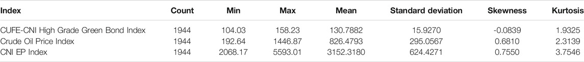
TABLE 1. The statistical description of three indexes
Methodology
In this paper, three machine learning models are used for forecasting the green bond index, which are CEEMDAN-LSTM, EMD-LSTM, and LSTM. When choosing our predictor variables, our paper takes the possible lagged correlations between the green bond market and other financial markets into consideration based on previous literature. In order to testify whether the crude oil index and the stock index are suitable predictors, following (Hou et al., 2018), we employ the Grey relational analysis to examine the correlations between the predictors and the next day’s closing price. Meanwhile, as the green bond index is unstable, the CEEMDAN and EMD are utilized to decompose the index into several sequences according to their frequency. Finally, after they are normalized, these time sequences are used to predict the future green bond trend with LSTM.
EMD
EMD is an adaptive signal time-frequency processing method (Huang et al., 1998). It decomposes the time series into a number of IMFs, according to the time scale feature of data. EMD is widely used in predicting stock price (Wang and Wang, 2017, Rezaei et al., 2021), sovereign bond yield (Wang et al., 2017), and crude oil price (Yu et al., 2008; Zhang et al., 2009).
The specific decomposition process of EMD is as follows. First, for an original data sequence
where
CEEMDAN
Although EMD does well in decomposing time series and has the adaptability to process data with complex structure, this method was criticized for its mode mixing effect. In order to solve this problem, Ensemble Empirical Mode Decomposition (EEMD) was proposed when the normally distributed white noise is added to the original sequence, largely eliminating mode mixing in EMD (Wu and Huang, 2009); but at the same time, this method has a new problem, that is, white noise cannot be completely cancelled after lumped average, resulting in reconstruction errors. Therefore, CEEMDAN was put forward by Torres et al. (2011), which adds adaptive noise to each component decomposed by EEMD, settling down the mode mixing and reconstruction errors simultaneously. Similarly, the CEEMDAN method has many applications in the studying stock market (Jothimani and Yadav, 2019), commodity market (Li et al., 2019; Zhou et al., 2019), and sovereign credit default swap market (Li et al., 2021).
Different from EMD, the Gaussian white noise sequence with standard normal distribution
The decomposing process is then performed to obtain the first
After obtaining the residue, the second component is expressed as follows:
where
And for the remaining process
LSTM
As is mentioned above, LSTM is a developed type of RNNs. Compared with other neutral networks, RNN allows information to persist for a long time, making it possible to use historical information. But RNN has the problem of long-term dependencies, which means the gradient vanishing would occur when the time sequence is long (Bengio et al., 1994). LSTM, which is capable of learning long-term series, was proposed to settle down the problem, (Hochreiter and Schmidhuber, 1997). It adds memory units to each neural unit of hidden layer, so that the memory information of time series can be controlled. Because of its unique structure, it is more suitable for processing and predicting time series problems. Thus, it is widely applied in analyzing financial markets (Kim and Won, 2018; Livieris et al., 2020; Vidal and Kristjanpoller, 2020). The calculation process can be separated into the following steps.
First, put data into forget gate and determine what should be discarded. At time
At the same time, calculate the value of the input gate to determine the new inputs that need to be retained. We use the input gate to update the value and a tanh layer to create a vector of new candidate values.
Then the memory cell
Finally, get the final outputs through the forget gate. We use the output gate to determine what kind of state values will be output. Then we use a tanh activation function to calculate the candidate value of current state value
The cell structure of LSTM is shown in Figure 2.
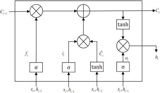
FIGURE 2. The structure of the LSTM cell.
Grey relational analysis
The Grey relational analysis method is used to measure the correlations among factors according to the degree of similarity. It has no requirements on sample size and statistical rules, so it is a common method when studying the relationship between variables (Feng et al., 2009). For example, Malinda and Chen (2021) use the Grey relational analysis method in predicting consumer exchange-traded funds (ETFs) and find four main factors influencing consumer ETFs from eight different variables, which are EUR/USD exchange rate, Commodity Research Bureau Index, New York Stock Exchange Composite Index, and put/call ratio. In addition, Chen et al. (2014) utilize Grey relational analysis and artificial neural network to predict the return of real estate investment trust and find that Grey relational analysis is of great significance in correcting predication errors.
The calculation process of this method is as follows. First, determine the reference sequence that reflects the characteristics of the system behavior and the comparison sequences that affect the system behavior. Then, make the reference sequence and comparison sequence dimensionless and calculate the Grey relational coefficient between reference sequence
The Grey relational coefficient
where
After that, we calculate the correlation level
Integrated forecasting model
Most previous literature have confirmed that the combined CEEMDAN-LSTM model have excellent performance in financial series prediction (Hu, 2021; Wang et al., 2021; Weng et al., 2021). In this paper, we also apply Grey relational analysis, CEEMDAN, and LSTM into the prediction of the green bond Index. The flow chart of our integrated forecasting model is presented in Figure 3. First, based on the previous literature, we have chosen five trading indicators of the green bond index as the predictors (closing price, opening price, volume, turnover of trading volumes, and daily return rate). Considering the dynamic correlations between the green bond market and other financial markets, we innovatively introduce the crude oil index and green stock index as predictors as well. After that, the Grey relational analysis is used to testify whether the predictors we choose are capable of predicting the green bond index. In this part, we use the closing price as the reference sequence and the lagged predictors as the comparison sequences to examine the correlations between them. If the correlations are significant, it means that the closing price is closely related to the first lag of predictors, suggesting our predictors can be used to predict the bond index ahead of time.
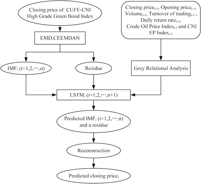
FIGURE 3. The flowchart of our integrated forecasting model.
At the same time, in order to stabilize the green bond index, we use CEEMDAN and EMD to decompose the index, respectively. This index is decomposed into several IMFs with different signal frequency and a residue that stands for the trend. These sequences are then used as the inputs of LSTM model. After the predicted sequences are output from LSTM, the forecasted green bond index can be obtained by summing up the predicted IMF sequences and the predicted residue sequence, as follows:
where
Before testing the prediction ability of our LSTM model, we have to train the model first. In this study, we divide our dataset into two parts: 80% of the data serve as the training data and the remaining 20% are used for out-of-sample prediction. In order to select the optimal model, we have built up three models in this paper: CEEMDAN-LSTM, EMD-LSTM, and LSTM model. These three models differ in the data processing of the green bond index. In CEEMDAN-LSTM and EMD-LSTM models, the predicted sequences are the IMFs and residue decomposed by CEEMDAN or EMD, respectively, while in the LSTM model, the original green bond index is used as the predicted sequence directly.
Evaluation criteria
Prediction accuracy means the similarity between the predicted value and the actual value. The closer the predicted value is to the actual value, the higher the prediction accuracy is. Following (Huang et al., 2005; Cao et al., 2019), we adopt four loss functions (MSE, RMSE, MAE, and MAPE) to evaluate the accuracy of different prediction models.
We use
1) Mean square error (MSE) represents the mean of squares of the distances between each predicted value and the actual value. The greater the MSE is, the greater the errors are.
2) RMSE stands for root mean square error. The relationship between MSE and RMSE is similar to the difference between variance and standard deviation.
3) Mean absolute error (MAE) is similar to RMSE and represents the mean of absolute value of the distances between each predicted value and the actual value.
4) Mean absolute percentage error (MAPE) compares the difference between the predicted value and the actual value to the actual value to see how much it is accounted for.
Empirical results
The result of Grey relational analysis
In order to evaluate whether the predictors we utilize are reasonable, we apply the method of Grey relational analysis to testify the relationships between one-day-lagged predictors and the closing price of the green bond index. Table 2 shows the result of Grey relational analysis, presenting that the Grey relational grades of these seven indicators are all above 0.75. It proves that the lagged variables are closely related to the closing price. Among the predictors, the lagged closing price and the lagged opening price are highly correlated with the closing price. It means that there exists first-order auto correlation in the closing price series. Therefore, we are able to predict the future trends of the green bond index based on historical data. Besides, the relationships between the closing price and other trading indicators are also demonstrated. It is worth noticing that the lagged crude oil index and lagged stock index are both closely related to the green bond index, indicating that the price changes in the crude oil market and green stock market will exert influence on the next day’s green bond market. Therefore, it is reasonable to dig out relationships between green bond markets and other financial markets. In a word, the predictors we select are highly related to the next day’s closing price of green bond index, which means they would lead the green bond market to a certain extent and can be used in the prediction of CUFE-CNI High Grade Green Bond Index.

TABLE 2. The results of Grey relational analysis on predictors
EMD and CEEMDAN methods
The EMD and CEEMDAN methods are widely applied in decomposing time series. Since (Huang et al., 2005) first introduced EMD to predict the stock price, many studies have utilized it to decompose the financial time series into several sequences for predicting various financial markets. CEEMDAN is later raised based on EMD to mitigate mode mixing and reduce noise. Compared with the original sequence, the decomposed sequences are more stable and smoother, which can be predicted more accurately. In our study, we use CEEMDAN and EMD, respectively, to decompose the CUFE-CNI High Grade Green Bond Index into five IMFs and a residue. These components are later used to predict the index through LSTM.
As is shown in Figures 4, 5, IMFs with higher frequency are placed at the higher places. In fact, the high-frequency sequences are often viewed as the noise in the green bond market, while the low-frequency sequences represent the fluctuations. Also, the residue representing the basic trend of the green bond index is arranged at the bottom of two figures. Table 3 gives a brief statistical description of the IMFs decomposed by CEEMDAN. It can be seen that all IMFs pass the Augmented Dickey-Fuller test under the statistical significance of 1%, suggesting they are all stationary series.
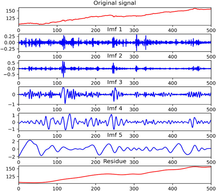
FIGURE 4. The IMFs decomposed by CEEMDAN.
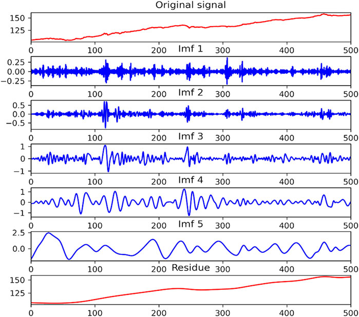
FIGURE 5. The IMFs decomposed by EMD.
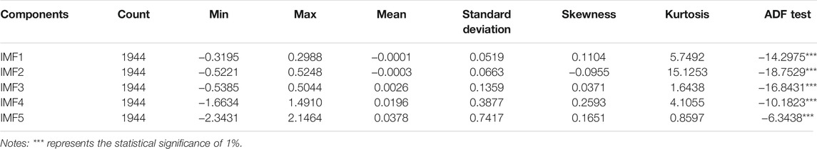
TABLE 3. The statistical description of IMFs
Training process and the results
After decomposing, the IMFs are supposed to be normalized before training. In this study, we use the following normalization equation:
where
To get the optimal predicted green bond index, we have trained the model many times, and the parameters are set as follows. In the process of CEEMDAN decomposing, the number of white noise trials is 50. As for the hyper-parameters in LSTM, after many experiments, we finally choose the number of epochs, which is the total times of training, as 175; and the figure of batch size, which refers to the samples captured in one training session is 64. In the first of hidden layer, the number of neurons is 50 and there is 1 neuron in the output layer to predict the closing price.
Figures 6–8 present the predicted curves of the CUFE-CNI High Grade Green Bond Index, through CEEMDAN-LSTM, EMD-LSTM, and LSTM models, respectively. It is transparent that, compared with original series, IMFs obtained through the CEEMDAN and EMD methods could be used to predict the future trend better. From Figure 8, we can see that the predicted curve of LSTM is of high volatility, suggesting there are more noise signals that weaken the accuracy of predicted value. Meanwhile, CEEMDAN-LSTM and EMD-LSTM all perform relatively well in forecasting, which means the prediction accuracy can be significantly enhanced when the original series is decomposed according to the signal frequency.
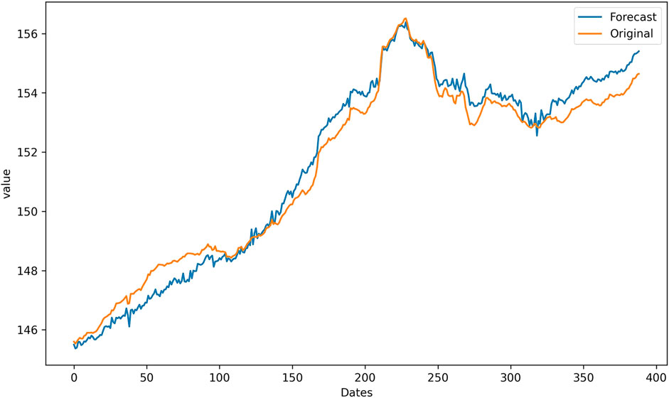
FIGURE 6. The forecasting results based on CEEMDAN-LSTM.
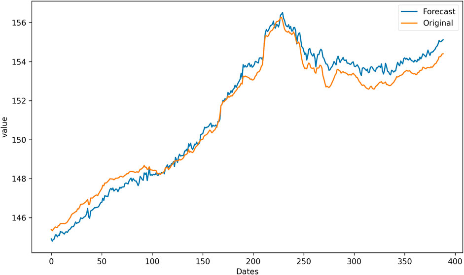
FIGURE 7. The forecasting results based on EMD-LSTM.
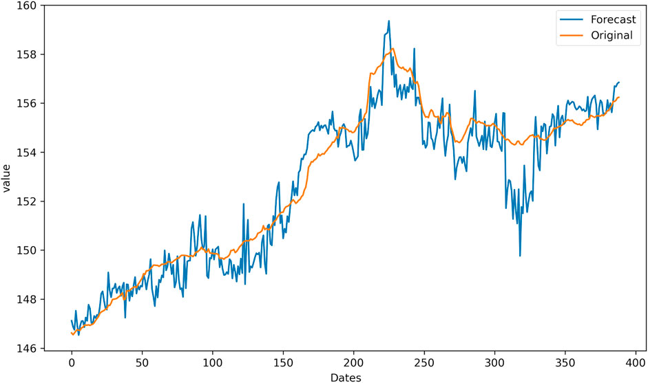
FIGURE 8. The forecasting results based on LSTM.
However, since CEEMDAN-LSTM and EMD-LSTM all have good performance in predicting, we apply four loss functions to compare these two models’ predicting abilities, and the result is suggested in Table 4. The four forecasting criteria we have chosen are MSE, RMSE, MAE, and MAPE. By contrasting forecasting errors of the CEEMDAN-LSTM and EMD-LSTM models, we can easily draw the conclusion that CEEMDAN-LSTM is the optimal method. No matter what kind of loss functions are used to evaluate the prediction performance, the CEEMDAN-LSTM model has the highest forecasting accuracy rate. In addition, the RMSE of the CEEMDAN-LSTM model suggests that on average, the difference between the predicted value and the actual value of the CUFE-CNI High Grade Green Bond Index is 0.267635. Therefore, our CEEMDAN-LSTM model can predict the closing price of the CUFE-CNI High Grade Green Bond Index to a large extent. Figure 9 shows the predicted closing price of the CUFE-CNI High Grade Green Bond Index based on the CEEMDAN-LSTM model. By contrasting the predicted value and the actual closing price presented in Figure 1, we find our model fit the CUFE-CNI High Grade Green Bond Index well. Therefore, the CEEMDAN-LSTM model performs well in forecasting the green bond index.
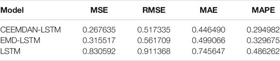
TABLE 4. The results of prediction using LSTM, EMD-LSTM, and CEEMDAN-LSTM
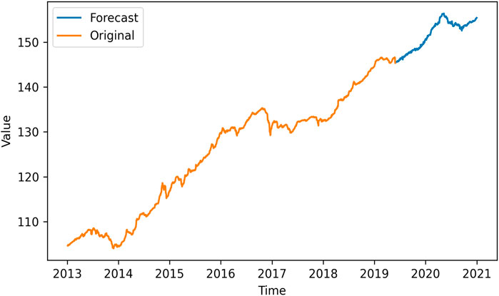
FIGURE 9. The predicted CUFE-CNI High Grade Green Bond Index based on CEEMDAN-LSTM.
Further discussion
The relationships between the green bond market and other financial markets have been heatedly discussed by lots of studies. Some papers suggest the correlation is weak (Reboredo and Ugolini, 2020), while others hold the opposite opinion (Dutta and Noor, 2021). Our work also partly answers the question by testing the predicting ability of other markets’ indices. When choosing predictors, we also take the price indices of the crude oil market and green stock market into account. Table 5 compares the forecasting results when the Crude Oil Price Index and CNI EP index are employed or not. It is shown that when Crude Oil Price Index and CNI EP Index are used as predictors, the forecasting performance of CEEMDAN-LSTM can be greatly improved.
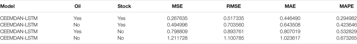
TABLE 5. The results of prediction when the Crude oil Price Index and CNI EP Index are used or not
In Table 6, we give a further analysis on the prediction performance that improved when the Crude Oil Price Index and the CNI EP Index served as the indicators. We can find that if the two indices are not included, the values of the loss functions MSE, RMSE, MAE, and MAPE of the CEEMDAN-LSTM model are 1.211728, 1.100785, 1.023617, and 0.673265 correspondingly. A new indicator
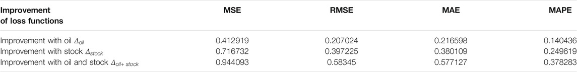
TABLE 6. The improvements when different indexes are added in the model
Conclusion
As ESG is attached with greater importance, many financial products designed to help environment-friendly projects are emerging. Green bond, serving as an innovative fixed-income asset, has been appealing to a majority of investors. However, this kind of financial instrument does not exist until 2007, which leads to the limited studies about it. Up to now, the prediction of the green bond market is still a research gap.
Previous literature has illustrated that machine methods (especially LSTM) perform better in terms of financial market prediction, and the prediction accuracy would be enhanced when the data are decomposed by CEEMDAN. Motivated by these studies, our paper proposes a hybrid CEEMDAN-LSTM model to forecast the green bond index (represented by the CUFE-CNI High Grade Green Bond Index). As for the predictor variables, we mainly utilize several technical predictors, including the closing price, the opening price, the trading volume, the turnover of trading volumes, and daily return rate. Considering the potential correlations between green bond market and other financial markets, we also try to use indices from the crude oil market and environmental stock market to forecast the green bond index. To examine the performance of our mixed CEEMDAN-LSTM model, we also apply the EMD-LSTM model and the LSTM model to predict the index.
Our empirical results suggest that compared with the other two models, our CEEMDAN-LSTM model is optimal with considerably high prediction accuracy, which demonstrates the powerful prediction ability of machine learning methods. Besides, our study also shows that the crude oil market and the environmental stock market could exert influence on the green bond market, implying the correlations among these three markets. The indices of these two markets can be used in green bond market forecasting.
Given our findings, several policy implications are put forward as follows:
(a) The rapid development of green bonds will definitely fuel the sustainable economy, which is especially significant for a developing country like China to seize the opportunity and promote the green investment.
(b) Our study has shown that the green bond index could be predicted considerably accurately through historical information. However, the trading information of the bond market is relatively inadequate compared with the stock market, resulting in the difficulty to forecast the future trend. Therefore, it is of great importance to set up the comprehensive information disclosure mechanism in the green bond market, which would also enable investors to green their portfolios effectively.
(c) As demonstrated in our work and previous literature, the green bond market could receive sizeable influence from other markets (e.g., crude oil market, stock market), suggesting the potential risk contagion among financial markets. Thus, more suitable government regulations are supposed to be implemented in order to monitor the financial contagion.
Data Availability Statement
The original contributions presented in the study are included in the article/Supplementary Material; further inquiries can be directed to the corresponding author.
Author Contributions
JW: Conceptualization, Data Curation, Methodology, Software, Formal analysis, Investigation, Writing-original draft, Visualization. JT: Conceptualization, Investigation, Writing-original draft, Visualization. KG: Conceptualization, Methodology, Investigation, Writing-review and editing, Supervision.
Funding
This research was funded by the University of Chinese Academy of Sciences and the Fundamental Research Funds for the Central Universities.
Conflict of Interest
The authors declare that the research was conducted in the absence of any commercial or financial relationships that could be construed as a potential conflict of interest.
Publisher’s Note
All claims expressed in this article are solely those of the authors and do not necessarily represent those of their affiliated organizations, or those of the publisher, the editors, and the reviewers. Any product that may be evaluated in this article, or claim that may be made by its manufacturer, is not guaranteed or endorsed by the publisher.
Supplementary Material
The Supplementary Material for this article can be found online at: https://www.frontiersin.org/articles/10.3389/fenrg.2021.793413/full#supplementary-material
References
Akita, R., Yoshihara, A., Matsubara, T., and Uehara, K. (2016). “Deep Learning for Stock Prediction Using Numerical and Textual Information,” in International Conference on Computer and Information Science (ICIS) (Okayama, Japan: IEEE), 1–6. doi:10.1109/ICIS.2016.7550882
Al-Thelaya, K. A., El-Alfy, E.-S. M., and Mohammed, S. (2019). “Forecasting of bahrain Stock Market with Deep Learning: Methodology and Case Study,” in 2019 8th International Conference on Modeling Simulation and Applied Optimization (ICMSAO), 1–5. doi:10.1109/ICMSAO.2019.8880382
Assis, C. A. S., Pereira, A. C. M., Carrano, E. G., Ramos, R., and Dias, W. (2018). “Restricted Boltzmann Machines for the Prediction of Trends in Financial Time Series,” in 2018 International Joint Conference on Neural Networks (IJCNN), 1–8. doi:10.1109/IJCNN.2018.8489163
Bauer, M. D., and Rudebusch, G. D. (2017). Resolving the Spanning Puzzle in Macro-Finance Term Structure Models*. Rev. Finance 21 (2), 511–553. doi:10.1093/rof/rfw044
Bengio, Y., Simard, P., and Frasconi, P. (1994). Learning Long-Term Dependencies with Gradient Descent Is Difficult. IEEE Trans. Neural Netw. 5 (2), 157–166. doi:10.1109/72.279181
Besley, T., and Ghatak, M. (2007). Retailing Public Goods: The Economics of Corporate Social Responsibility. J. Public Econ. 91 (9), 1645–1663. doi:10.1016/j.jpubeco.2007.07.006
Bezerra, P. C. S., and Albuquerque, P. H. M. (2017). Volatility forecasting via SVR–GARCH with mixture of Gaussian kernels. Comput. Manag. Sci. 14 (2), 179–196. doi:10.1007/s10287-016-0267-0
Bianchi, D., Büchner, M., and Tamoni, A. (2021). Bond Risk Premiums with Machine Learning. Rev. Financial Stud. 34 (2), 1046–1089. doi:10.1093/rfs/hhaa062
Bracking, S. (2015). Performativity in the Green Economy: How Far Does Climate Finance Create a Fictive Economy? Third World Q. 36 (12), 2337–2357. doi:10.1080/01436597.2015.1086263
Cao, J., Li, Z., and Li, J. (2019). Financial Time Series Forecasting Model Based on CEEMDAN and LSTM. Physica A: Stat. Mech. its Appl. 519, 127–139. doi:10.1016/j.physa.2018.11.061
Chen, J.-H., Chang, T.-T., Ho, C.-R., and Diaz, J. F. (2014). Grey Relational Analysis and Neural Network Forecasting of REIT Returns. Quantitative Finance 14 (11), 2033–2044. doi:10.1080/14697688.2013.816765
Chen, L., Chi, Y., Guan, Y., and Fan, J. (2019). “A Hybrid Attention-Based EMD-LSTM Model for Financial Time Series Prediction,” in 2019 2nd International Conference on Artificial Intelligence and Big Data (ICAIBD), 113–118. doi:10.1109/ICAIBD.2019.8837038
Chen, Y., and Zhao, Z. J. (2021). The Rise of green Bonds for Sustainable Finance: Global Standards and Issues with the Expanding Chinese Market. Curr. Opin. Environ. Sustainability 52, 54–57. doi:10.1016/j.cosust.2021.06.013
Choi, J., and Kim, Y. (2018). Anomalies and Market (Dis)integration. J. Monetary Econ. 100, 16–34. doi:10.1016/j.jmoneco.2018.06.003
Chordia, T., Goyal, A., Nozowa, Y., Subrahmanyam, A., and Tong, Q. (2014). Is the Cross-Section of Expected Bond Returns Influenced by Equity Return Predictors? Res. Collection Lee Kong Chian Sch. Business. Available at: https://ink.library.smu.edu.sg/lkcsb_research/4521.
Christophers, B. (2019). Environmental Beta or How Institutional Investors Think about Climate Change and Fossil Fuel Risk. Ann. Am. Assoc. Geogr. 109 (3), 754–774. doi:10.1080/24694452.2018.1489213
Climate Bonds Initiative (2018). Bonds and Climate Change: State of the Market. Available at: http://www.climatebonds.net/resources/reports/green-bonds-state-market-2018 (Accessed October 10, 2021).
Climate Bonds Initiative (2020). China State of the Market 2020 Report. Available at: http://www.climatebonds.net/resources/reports/china-state-market-2020-report (Accessed November 25, 2021).
Climate Bonds Initiative (2021). Sustainable Debt Highlights H1 2021. Available at: http://www.climatebonds.net/resources/reports/sustainable-debt-highlights-h1-2021 (Accessed November 25, 2021).
Colominas, M. A., Schlotthauer, G., and Torres, M. E. (2014). Improved Complete Ensemble EMD: A Suitable Tool for Biomedical Signal Processing. Biomed. Signal Process. Control. 14, 19–29. doi:10.1016/j.bspc.2014.06.009
Connolly, R., Stivers, C., and Sun, L. (2005). Stock Market Uncertainty and the Stock-Bond Return Relation. J. Financ. Quant. Anal. 40 (1), 161–194. doi:10.1017/S0022109000001782
Devpura, N., Narayan, P. K., and Sharma, S. S. (2021). Bond Return Predictability: Evidence from 25 OECD Countries. J. Int. Financial Markets, Institutions Money 75, 101301. doi:10.1016/j.intfin.2021.101301
Dingli, A., Fournier, K. S., and Fournier, K. S. (2017). Financial Time Series Forecasting - A Deep Learning Approach. Int. J. Machine Learn. Comput. 7 (5), 118–122. doi:10.18178/ijmlc.2017.7.5.632
Dutta, A., Bouri, E., and Noor, M. H. (2021). Climate Bond, Stock, Gold, and Oil Markets: Dynamic Correlations and Hedging Analyses during the COVID-19 Outbreak. Resour. Pol. 74, 102265. doi:10.1016/j.resourpol.2021.102265
Febi, W., Schäfer, D., Stephan, A., and Sun, C. (2018). The Impact of Liquidity Risk on the Yield Spread of green Bonds. Finance Res. Lett. 27, 53–59. doi:10.1016/j.frl.2018.02.025
Feng, D., Qingmei, T., and Xiaohui, L. (2009). “The Relationship between Chinese Energy Consumption and GDP: An Econometric Analysis Based on the Grey Relational Analysis(GRA),” in 2009 IEEE International Conference on Grey Systems and Intelligent Services (GSIS 2009) (Nanjing, China: IEEE), 153–157. doi:10.1109/GSIS.2009.5408333
Flammer, C. (2021). Corporate green Bonds. J. Financial Econ. 142, 499–516. doi:10.1016/j.jfineco.2021.01.010
Fong, T. P. W., and Wu, S. T. (2020). Predictability in Sovereign Bond Returns Using Technical Trading Rules: Do Developed and Emerging Markets Differ? North Am. J. Econ. Finance 51, 101105. doi:10.1016/j.najef.2019.101105
Friede, G., Busch, T., and Bassen, A. (2015). ESG and Financial Performance: Aggregated Evidence from More Than 2000 Empirical Studies. J. Sustain. Finance Investment 5 (4), 210–233. doi:10.1080/20430795.2015.1118917
Ganguli, S., and Dunnmon, J. (2017). Machine Learning for Better Models for Predicting Bond Prices. arXiv preprint arXiv:1705.01142. Available at: https://arxiv.abs/1705.01142.
Gao, T., and Chai, Y. (2018). Improving Stock Closing price Prediction Using Recurrent Neural Network and Technical Indicators. Neural Comput. 30 (10), 2833–2854. doi:10.1162/neco_a_01124
Ghoddusi, H., Creamer, G. G., and Rafizadeh, N. (2019). Machine Learning in Energy Economics and Finance: A Review. Energ. Econ. 81, 709–727. doi:10.1016/j.eneco.2019.05.006
Giacoletti, M., Laursen, K. T., and Singleton, K. J. (2021). Learning from Disagreement in the U.S. Treasury Bond Market. J. Finance 76 (1), 395–441. doi:10.1111/jofi.12971
Gite, S., Khatavkar, H., Kotecha, K., Srivastava, S., Maheshwari, P., and Pandey, N. (2021). Explainable Stock Prices Prediction from Financial News Articles Using Sentiment Analysis. PeerJ Comput. Sci. 7, e340. doi:10.7717/peerj-cs.340
Gormus, A., Nazlioglu, S., and Soytas, U. (2018). High-yield Bond and Energy Markets. Energ. Econ. 69, 101–110. doi:10.1016/j.eneco.2017.10.037
Gu, S., Kelly, B., and Xiu, D. (2020). Empirical Asset Pricing via Machine Learning. Rev. Financial Stud. 33 (5), 2223–2273. doi:10.1093/rfs/hhaa009
Hachenberg, B., and Schiereck, D. (2018). Are green Bonds Priced Differently from Conventional Bonds? J. Asset Manag. 19 (6), 371–383. doi:10.1057/s41260-018-0088-5
Hammoudeh, S., Ajmi, A. N., and Mokni, K. (2020). Relationship between green Bonds and Financial and Environmental Variables: A Novel Time-Varying Causality. Energ. Econ. 92, 104941. doi:10.1016/j.eneco.2020.104941
Henrique, B. M., Sobreiro, V. A., and Kimura, H. (2019). Literature Review: Machine Learning Techniques Applied to Financial Market Prediction. Expert Syst. Appl. 124, 226–251. doi:10.1016/j.eswa.2019.01.012
Hochreiter, S., and Schmidhuber, J. (1997). Long Short-Term Memory. Neural Comput. 9 (8), 1735–1780. doi:10.1162/neco.1997.9.8.1735
Hou, X., Zhu, S., Xia, L., and Wu, G. (2018). “Stock price Prediction Based on Grey Relational Analysis and Support Vector Regression,” in 2018 Chinese Control and Decision Conference (CCDC) (Shenyang, China: IEEE), 2509–2513. doi:10.1109/CCDC.2018.8407547
Hsu, M.-W., Lessmann, S., Sung, M.-C., Ma, T., and Johnson, J. E. V. (2016). Bridging the divide in Financial Market Forecasting: Machine Learners vs. Financial Economists. Expert Syst. Appl. 61, 215–234. doi:10.1016/j.eswa.2016.05.033
Hu, Z. (2021). Crude Oil price Prediction Using CEEMDAN and LSTM-Attention with News Sentiment index. Oil Gas Sci. Technol. - Rev. IFP Energies Nouvelles 76, 28. doi:10.2516/ogst/2021010
Huang, D., Jiang, F., Tong, G., Tong, G., and Zhou, G. (2020). “Real Time Macro Factors in Bond Risk Premium, SSRN Journal,” in Asian Finance Association (AsianFA) 2018 Conference. doi:10.2139/ssrn.3107612
Huang, N. E., Shen, Z., Long, S. R., Wu, M. C., Shih, H. H., Zheng, Q., et al. (19981971). The Empirical Mode Decomposition and the Hilbert Spectrum for Nonlinear and Non-stationary Time Series Analysis. Proc. R. Soc. Lond. A. 454, 903–995. doi:10.1098/rspa.1998.0193
Huang, W., Nakamori, Y., and Wang, S.-Y. (2005). Forecasting Stock Market Movement Direction with Support Vector Machine. Comput. Operations Res. 32 (10), 2513–2522. doi:10.1016/j.cor.2004.03.016
Huynh, H. D., Dang, L. M., and Duong, D. (2017). “A New Model for Stock Price Movements Prediction Using Deep Neural Network,” in Proceedings of the Eighth International Symposium on Information and Communication Technology, 57–62. doi:10.1145/3155133.3155202
Jiang, W. (2021). Applications of Deep Learning in Stock Market Prediction: Recent Progress. Expert Syst. Appl. 184, 115537. doi:10.1016/j.eswa.2021.115537
Jothimani, D., and Yadav, S. S. (2019). Stock Trading Decisions Using Ensemble-Based Forecasting Models: a Study of the Indian Stock Market. J. Bank Financ. Technol. 3, 113–129. doi:10.1007/s42786-019-00009-7
Kamal, I. M., Bae, H., Sunghyun, S., and Yun, H. (2020). DERN: Deep Ensemble Learning Model for Short- and Long-Term Prediction of Baltic Dry Index. Appl. Sci. 10 (4), 1504. doi:10.3390/app10041504
Khan, M., Serafeim, G., and Yoon, A. (2016). Corporate Sustainability: First Evidence on Materiality. Account. Rev. 91 (6), 1697–1724. doi:10.2308/accr-51383
Kim, H. Y., and Won, C. H. (2018). Forecasting the Volatility of Stock price index: A Hybrid Model Integrating LSTM with Multiple GARCH-type Models. Expert Syst. Appl. 103, 25–37. doi:10.1016/j.eswa.2018.03.002
Kim, J.-M., Kim, D. H., and Jung, H. (2021). Applications of Machine Learning for Corporate Bond Yield Spread Forecasting. North Am. J. Econ. Finance 58, 101540. doi:10.1016/j.najef.2021.101540
Kochetygova, J., and Jauhari, A. (2014). Climate Change, green Bonds and index Investing: the New Frontier. Retrieved, 20, 2017. Available at: https://www.spglobal.com/spdji/en/documents/research/research-climate-change-green-bonds-and-index-investing-the-new-frontier.pdf.
Kumar, M., and Thenmozhi, M. (2014). Forecasting Stock index Returns Using ARIMA-SVM, ARIMA-ANN, and ARIMA-Random forest Hybrid Models. Int. J. Banking Account. Finance 5 (3), 284–308. doi:10.1504/IJBAAF.2014.064307
Lesmond, D. A., Ogden, J. P., and Trzcinka, C. A. (1999). A New Estimate of Transaction Costs. Rev. Financ. Stud. 12 (5), 1113–1141. doi:10.1093/rfs/12.5.1113
Li, J., Hao, J., Sun, X., and Feng, Q. (2021). Forecasting China’s sovereign CDS with a decomposition reconstruction strategy. Appl. Soft. Comput. 105, 107291. doi:10.1016/j.asoc.2021.107291
Li, T., Zhou, Y., Li, X., Wu, J., and He, T. (2019). Forecasting Daily Crude Oil Prices Using Improved CEEMDAN and ridge Regression-Based Predictors. Energies 12 (19), 3603. doi:10.3390/en12193603
Li, Y., and Ma, W. (2010). “Applications of Artificial Neural Networks in Financial Economics: a Survey,” in 2010 International symposium on computational intelligence and design (Hangzhou, China: IEEE), 211–214. doi:10.1109/ISCID.2010.70
Liaw, K. T. (2020). Survey of Green Bond Pricing and Investment Performance. J. Risk Financial Manage. 13 (9), 193. doi:10.3390/jrfm13090193
Lin, H., Wu, C., and Zhou, G. (2018). Forecasting Corporate Bond Returns with a Large Set of Predictors: An Iterated Combination Approach. Manage. Sci. 64 (9), 4218–4238. doi:10.1287/mnsc.2017.2734
Lin, Y., Yan, Y., Xu, J., Liao, Y., and Ma, F. (2021). Forecasting Stock index price Using the CEEMDAN-LSTM Model. North Am. J. Econ. Finance 57, 101421. doi:10.1016/j.najef.2021.101421
Livieris, I. E., Pintelas, E., and Pintelas, P. (2020). A CNN-LSTM Model for Gold price Time-Series Forecasting. Neural Comput. Applic 32 (23), 17351–17360. doi:10.1007/s00521-020-04867-x
Malinda, M., and Chen, J.-H. (2021). The Forecasting of Consumer Exchange-Traded Funds (ETFs) via Grey Relational Analysis (GRA) and Artificial Neural Network (ANN). Empir Econ. 2021, 1–45. doi:10.1007/s00181-021-02039-x
Nazlioglu, S., Gupta, R., and Bouri, E. (2020). Movements in International Bond Markets: The Role of Oil Prices. Int. Rev. Econ. Finance 68, 47–58. doi:10.1016/j.iref.2020.03.004
Orlitzky, M., Siegel, D. S., and Waldman, D. A. (2011). Strategic Corporate Social Responsibility and Environmental Sustainability. Business Soc. 50 (1), 6–27. doi:10.1177/0007650310394323
Partridge, C., and Medda, F. (2018). The Creation and Benchmarking of a green Municipal Bond index. SSRN J. Available at SSRN 3248423. doi:10.2139/ssrn.3248423
Pham, L., and Luu Duc Huynh, T. (2020). How Does Investor Attention Influence the green Bond Market? Finance Res. Lett. 35, 101533. doi:10.1016/j.frl.2020.101533
Piñeiro-Chousa, J., López-Cabarcos, M. Á., Caby, J., and Šević, A. (2021). The Influence of Investor Sentiment on the green Bond Market. Technol. Forecast. Soc. Change 162, 120351. doi:10.1016/j.techfore.2020.120351
Reboredo, J. C. (2018). Green Bond and Financial Markets: Co-movement, Diversification and price Spillover Effects. Energ. Econ. 74, 38–50. doi:10.1016/j.eneco.2018.05.030
Reboredo, J. C., and Ugolini, A. (2020). Price Connectedness between green Bond and Financial Markets. Econ. Model. 88, 25–38. doi:10.1016/j.econmod.2019.09.004
Rezaei, H., Faaljou, H., and Mansourfar, G. (2021). Stock price Prediction Using Deep Learning and Frequency Decomposition. Expert Syst. Appl. 169, 114332. doi:10.1016/j.eswa.2020.114332
Sadorsky, P. (2021). A Random Forests Approach to Predicting Clean Energy Stock Prices. J. Risk Financial Manag. 14 (2), 48. doi:10.3390/jrfm14020048
Sanboon, T., Keatruangkamala, K., and Jaiyen, S. (2019). Singapore: IEEE, 757–760. doi:10.1109/CCOMS.2019.8821776 A Deep Learning Model for Predicting Buy and Sell Recommendations in Stock Exchange of Thailand Using Long Short-Term Memory2019 IEEE 4th International Conference on Computer and Communication Systems (ICCCS)
Sethia, A., and Raut, P. (2019). “Application of LSTM, GRU and ICA for Stock price Prediction,” in Information and Communication Technology for Intelligent Systems (Singapore: Springer), 479–487. doi:10.1007/978-981-13-1747-7_46
Shah, D., Isah, H., and Zulkernine, F. (2019). Stock Market Analysis: A Review and Taxonomy of Prediction Techniques. Int. J. Financial Stud. 7 (2), 26. doi:10.3390/ijfs7020026
Sheng, Q., Zheng, X., and Zhong, N. (2021). Financing for Sustainability: Empirical Analysis of green Bond Premium and Issuer Heterogeneity. Nat. Hazards 107, 2641–2651. doi:10.1007/s11069-021-04540-z
Sun, J., Xiao, K., Liu, C., Zhou, W., and Xiong, H. (2019). Exploiting Intra-day Patterns for Market Shock Prediction: A Machine Learning Approach. Expert Syst. Appl. 127, 272–281. doi:10.1016/j.eswa.2019.03.006
Tang, D. Y., and Zhang, Y. (2020). Do shareholders Benefit from green Bonds? J. Corporate Finance 61, 101427. doi:10.1016/j.jcorpfin.2018.12.001
Torres, M. E., Colominas, M. A., Schlotthauer, G., and Flandrin, P. (2011). “A Complete Ensemble Empirical Mode Decomposition with Adaptive Noise,” in 2011 IEEE International Conference on Acoustics, Speech and Signal Processing (ICASSP). doi:10.1109/ICASSP.2011.5947265
Trinks, A., Scholtens, B., Mulder, M., and Dam, L. (2018). Fossil Fuel Divestment and Portfolio Performance. Ecol. Econ. 146, 740–748. doi:10.1016/j.ecolecon.2017.11.036
Vidal, A., and Kristjanpoller, W. (2020). Gold Volatility Prediction Using a CNN-LSTM Approach. Expert Syst. Appl. 157, 113481. doi:10.1016/j.eswa.2020.113481
Vlasenko, A., Rashkevych, Y., Vlasenko, N., Peleshko, D., and Vynokurova, O. (2020). “A Hybrid EMD - Neuro-Fuzzy Model for Financial Time Series Analysis,” in 2020 IEEE Third International Conference on Data Stream Mining & Processing (DSMP) (Lviv, Ukraine: IEEE), 112–115. doi:10.1109/DSMP47368.2020.9204179
Wang, J., Sun, X., Cheng, Q., and Cui, Q. (2021). An Innovative Random forest-based Nonlinear Ensemble Paradigm of Improved Feature Extraction and Deep Learning for Carbon price Forecasting. Sci. Total Environ. 762, 143099. doi:10.1016/j.scitotenv.2020.143099
Wang, J., Sun, X., and Li, J. (2017). How Does Economic Policy Uncertainty Interact with Sovereign Bond Yield? Evidence from the US. Proced. Comput. Sci. 122, 154–158. doi:10.1016/j.procs.2017.11.354
Weng, Y., Wang, Z., and Zhou, L. (2021). LSTM Framework Design and Volatility Research on Intelligent Forecasting Model for Solving the Parallel Dislocation Problem. J. Phys. Conf. Ser. 1982 (1), 012028. doi:10.1088/1742-6596/1982/1/012028
World Bank Group (2015). What Are green Bonds? (English). Available at: https://documents.worldbank.org/en/publication/documents-reports/documentdetail/400251468187810398/what-are-green-bonds (Accessed November 24, 2021).
Wu, Z., and Huang, N. E. (2009). Ensemble Empirical Mode Decomposition: a Noise-Assisted Data Analysis Method. Adv. Adapt. Data Anal. 01 (01), 1–41. doi:10.1142/s1793536909000047
Xian, L., He, K., Wang, C., and Lai, K. K. (2020). Factor Analysis of Financial Time Series Using EEMD-ICA Based Approach. Sustainable Futures 2, 100003. doi:10.1016/j.sftr.2019.100003
Yu, L., Wang, S., and Lai, K. K. (2008). Forecasting Crude Oil price with an EMD-Based Neural Network Ensemble Learning Paradigm. Energ. Econ. 30 (5), 2623–2635. doi:10.1016/j.eneco.2008.05.003
Zerbid, O. D. (2019). The Effect of Pro-environmental Preferences on Bond Prices: Evidence from green Bonds. J. Bank. Financ. 98, 39–60. doi:10.1057/s41260-018-0088-5
Zhang, H. (2020). Regulating green Bond in China: Definition Divergence and Implications for Policy Making. J. Sustain. Finance Investment 10 (2), 141–156. doi:10.1080/20430795.2019.1706310
Zhang, N., Lin, A., and Shang, P. (2017). Multidimensionalk-nearest Neighbor Model Based on EEMD for Financial Time Series Forecasting. Physica A: Stat. Mech. its Appl. 477 (1), 161–173. doi:10.1016/j.physa.2017.02.072
Zhang, X., Yu, L., Wang, S., and Lai, K. K. (2009). Estimating the Impact of Extreme Events on Crude Oil price: An EMD-Based Event Analysis Method. Energ. Econ. 31 (5), 768–778. doi:10.1016/j.eneco.2009.04.003
Zhang, Y., Xiong, R., He, H., and Pecht, M. G. (2018). Long Short-Term Memory Recurrent Neural Network for Remaining Useful Life Prediction of Lithium-Ion Batteries. IEEE Trans. Veh. Technol. 67 (7), 5695–5705. doi:10.1109/TVT.2018.2805189
Zhong, X., and Enke, D. (2017). Forecasting Daily Stock Market Return Using Dimensionality Reduction. Expert Syst. Appl. 67, 126–139. doi:10.1016/j.eswa.2016.09.027
Zhou, Y., Li, T., Shi, J., and Qian, Z. (2019). A CEEMDAN and XGBOOST-Based Approach to Forecast Crude Oil Prices. Complexity 2019, 1–15. doi:10.1155/2019/4392785
Keywords: green bonds, CEEMDAN, LSTM, green finance, machine learning
Citation: Wang J, Tang J and Guo K (2022) Green Bond Index Prediction Based on CEEMDAN-LSTM. Front. Energy Res. 9:793413. doi: 10.3389/fenrg.2021.793413
Received: 12 October 2021; Accepted: 28 December 2021;
Published: 10 February 2022.
Edited by:
Xun Zhang, Academy of Mathematics and Systems Science (CAS), ChinaReviewed by:
Vidya C. T., Centre for Economic and Social Studies (CESS), IndiaJian Li Jane Hao, Xi’an Jiaotong-Liverpool University, China
Copyright © 2022 Wang, Tang and Guo. This is an open-access article distributed under the terms of the Creative Commons Attribution License (CC BY). The use, distribution or reproduction in other forums is permitted, provided the original author(s) and the copyright owner(s) are credited and that the original publication in this journal is cited, in accordance with accepted academic practice. No use, distribution or reproduction is permitted which does not comply with these terms.
*Correspondence: Kun Guo, Z3Vva3VuQHVjYXMuYWMuY24=