A Novel Decomposition and Combination Technique for Forecasting Monthly Electricity Consumption

With the share of electricity in total final energy consumption increasing quickly, the world is becoming increasingly dependent on electricity, which makes it more and more important to improve the forecasting accuracy of electricity consumption to ensure the normal operation of economic activities. In this paper, a novel decomposition and combination technique to forecast monthly electricity consumption is proposed. First, we use STL decomposition to obtain the trend, season, and residual components of the time series. Second, we use SARIMA, SVR, ANN, and LSTM to forecast trend, season, and residual component, respectively. Third, we use time correlation principle to improve the forecasting accuracy of season component. Fourth, we integrated the residual component predicted by SARIMA, SVR, ANN, and LSTM into a new sequence to improve the forecasting accuracy of residual component. In order to verify the performance of the proposed forecast model, monthly electricity consumption data in China is introduced as an example for empirical analysis. The results show that after STL decomposition, time correlation modification, and residual modification, the forecasting accuracy of each model has been gradually improved. We believe that the proposed forecast model in this paper can also be used to solve other mid- and long-term forecasting problems with obvious seasonal characteristics.

Introduction

Background

Resource depletion and global climate change are serious problems that human society is facing and will face for a long time. To escape from this dilemma, the global energy mix needs two transformations: clean energy substitution on the energy supply side and electric energy substitution on the energy consumption side. This paper focuses on electricity consumption. According to statistics, global electrification of the final consumption continues to follow an increasing trend, and the share of electricity in total final energy consumption is close to 20% in 2020.

As the world becomes more and more dependent on electricity, planning for electricity production is crucial. In addition, electricity is difficult to store, so it is usually used immediately after it is generated. This further increases the need for power companies to plan their electricity supply in a proactive manner. Reliable forecast of future electricity consumption level is the primary guiding principle of planning. In particular, high forecasting accuracy of medium- and long-term electricity consumption is the key to power system scheduling and planning. In contrast, inaccurate forecast of electricity consumption can backfire. Overestimation will waste scarce energy resources, huge capital investment, and long construction time. Underestimation will lead to more serious negative consequences, such as power shortage. Clearly, if effective early warning is given in advance based on high forecasting accuracy of electricity consumption, some measures can be adopted to avoid negative consequences. However, electricity consumption is uncertain, complex, and nonlinear, which depends on political conditions, economy (Lin and Liu, 2016), human activities, population behavior (Hussain et al., 2016), climate factors (Hernández, 2013), and other external factors affecting the forecasting accuracy of electricity consumption.

Literature Review and Motivation

At present, many techniques are used to forecast electricity consumption, which can be roughly divided into three categories: nonlinear intelligent model, statistical analysis model, and gray forecasting model. Nonlinear models mainly include the artificial neural network (Kandananond, 2011; Kaytez et al., 2015; Liu et al., 2017; Ghadimi et al., 2018; Bedi and Toshniwal, 2019; Hamzaçebi et al., 2019), support vector machine (Pai and Hong, 2005; Kavaklioglu, 2011; Cao and Wu, 2016), and Markov chain (Zhao et al., 2014). In addition to the nonlinear intelligent models mentioned above, statistical analysis models, such as regression analysis method (Mohamed and Bodger, 2005; Wang et al., 2018) and autoregressive integrated moving average (Yuan et al., 2016), have also been widely used in electricity consumption forecasting. The gray forecasting model proposed by Deng enjoys high popularity in many forecasting applications because it can describe the characteristics of uncertain systems even in the face of a small amount of data. Therefore, some literature forecast electricity consumption based on the gray model (Akay and Atak, 2007; Bahrami et al., 2014; Zhao and Guo, 2016; Xu et al., 2017; Ding et al., 2018; Wu et al., 2018).

These methods can generally provide good forecasts. However, the statistical analysis models have the limitation of linear (or near linear) assumption, the gray forecasting models are usually only suitable for time series that approximate exponential growth, and the nonlinear intelligent models often suffer from overfitting or the difficulty of parameter selection. To remedy these shortcomings, some decomposition and combination techniques have been proposed in recent years and achieve better performance: the SARIMA model with residual modification (Wang et al., 2012), wavelet transform combined with machine learning and time series models (Nguyen and Nabney, 2010), weighted hybrid model where trend and seasonal components are predicted by combined method, and SARIMA, respectively (Zhu, 2011), bagging ARIMA and exponential smoothing methods (de Oliveira and Cyrino Oliveira, 2018), convolutional neural networks and fuzzy time series (Sadaei et al., 2019), and structural combination of seasonal exponential smoothing forecasts (Rendon-Sanchez and de Menezes, 2019).

For the above existing researches, there are still some issues that need to be further studied. First, the statistical analysis models assume linearity and have good forecasting accuracy for periodic and regular sequences. The nonlinear intelligent model can forecast nonlinear and irregular time series better, but it has the problem of overfitting. How could the advantages of the two methods be combined to improve the forecasting accuracy? Second, except for the fluctuations of monthly electricity consumption affected by extreme weather changes, and sudden major economic and health events, the monthly electricity consumption also shows strong periodicity and regularity, so the comprehensive utilization of these two characteristics is meaningful to increase forecasting accuracy.

Contributions

To bridge the gap discussed above in the Literature review and motivation section, this paper develops a novel decomposition and combination forecasting technique. The primary research contents of this paper include three parts. First is the research on the monthly electricity consumption forecast based on STL decomposition. Second is the research on a time correlation modification based on annual periodicity and adjacent similarity to improve the forecasting accuracy of the season component. Third, considering the residual component has nonlinear and irregular characteristics, the individual model may only extract a certain feature of the sequence. Therefore, we integrate the residual component predicted by four models into a new sequence to improve the forecasting accuracy of the residual component. The main contributions of this paper are as follows:

1) A novel decomposition and combination forecasting model utilizing STL decomposition, time correlation principle (embodied as annual periodicity and adjacent similarity), and hybrid forecasting principle is proposed.

2) The monthly electricity consumption data of China are applied to evaluate the performance of the proposed model.

The remainder of the paper is organized as follows. The Electricity consumption month-ahead forecasting model section introduces the proposed forecasting model. The Case study section presents the simulation results and discussion, in which the performance of the proposed forecasting model is evaluated. Finally, conclusions are drawn in the Conclusion section.

Electricity Consumption Month-Ahead Forecasting Model

This section first briefly introduces individual models, including the STL algorithm, SARIMA, SVR, ANN, and LSTM model. Then the operation process of the proposed decomposition and combination method is described.

Seasonal–Trend Decomposition Using Loess Decomposition

For seasonal time series, academics generally use STL decomposition proposed by Cleveland et al. (1990) to obtain trend, season, and residual components. STL is a decompose model in the form of addition. In STL, loess is used to divide the time series into trend component, seasonal component, and residual component. Division is addition, that is, adding up the parts to get the original series. Specifically, the steps of STL decomposition are 1) detrending; 2) periodic subsequence smoothing: establish a sequence for each seasonal component and smooth it separately; 3) smoothing periodic substring low-pass filtering: recombine substring to smooth; 4) detrending the seasonal series; 5) detrending the original series using the seasonal components calculated in the previous steps; and 6) smoothing the de-seasonal sequence to obtain the trend component.

Seasonal Autoregressive Integrated Moving Average

SARIMA is one of the most widely used linear models for time series prediction. The general equation of this model is given by Eq. 1.

${\varphi }_p\left(\mathrm{B}\right){\left(1-B\right)}^d{\Phi }_P\left(B^s\right){\left(1-B^s\right)}^D{y}_t={\theta }_q\left(\mathrm{B}\right){\Theta }_Q\left(B^s\right)a_t.(1)$

Here $y_t$ is time series, $a_t$ is white noise, and B is the lag operator. D represents the seasonal differentiation order, and d represents the regular differentiation order.

${\varphi }_p\left(\mathrm{B}\right)=1-{\phi }_{1}B-{\phi }_2{B}^2-\dots -{\phi }_p{B}^p.(2)$

${\theta }_p\left(\mathrm{B}\right)=1-{\theta }_{1}B-{\theta }_2{B}^2-\dots -{\theta }_q{B}^q.(3)$

Eqs. 2, 3 represent the autoregressive and moving average polynomial, respectively. They represent the dependence of future values of time series on past values as well as errors.

${\Phi }_P\left(\mathrm{B}\right)=1-{\mu }_1{B}^S-{\mu }_2{B}^{2S}-\dots -{\mu }_P{B}^{PS}.(4)$

${\Theta }_Q\left(\mathrm{B}\right)=1-{\upsilon }_1{B}^S-{\nu }_2{B}^{2S}-\dots -{\nu }_P{B}^{QS}.(5)$

Similarly, Eqs. 4, 5 represent the seasonal autoregressive and seasonal moving average polynomials, respectively. Addition of these polynomials to the ARIMA equation helps in capturing the seasonal variation in time series. Differentiation is necessary for converting the nonstationary time series to a stationary one. S represents the order of seasonality.

Support Vector Machine

SVM was first proposed by Vapnik (1963) based on the statistical learning theory and principle of structural risk minimization, which possess good performance even for small samples. The basic idea of support vector regression is to map original data to high-dimensional feature space and perform linear regression in the space. It can be formulated into:

$f\left(x\right)=w^T\phi \left(x\right)+b,(6)$

where $\phi \left(x\right)$ is a nonlinear mapping function, $f\left(x\right)$ is the estimation value, and $w^T$ and b are weights. It can be translated into an optimization problem:

$\text{Min} \frac{1}{2}{w}^{T}w+C{\displaystyle \sum _{t=1}^T\left({\xi }_t+{\xi }_t^{\ast }\right)},$

$s.t\{\begin{array}{c}{w}^T\phi \left(x_t\right)+b-y_t\le \epsilon +{\xi }_t,\left(t=\mathrm{1,2},\dots ,T\right)\\ y_t-\left(w^T\phi \left(x_t\right)+b\right)\le \epsilon +{\xi }_t^{\ast },\left(t=\mathrm{1,2},\dots ,T\right)\\ {\xi }_t,{\xi }_t^{\ast }\ge 0\end{array},(7)$

where C is the penalty parameter, and ${\xi }_t$ and ${\xi }_t^{\ast }$ are the nonnegative slack variables. Generally speaking, the parameters of SVR have a great influence on the accuracy of the regression estimation. Thereby, the grid search method is employed to automatically choose the optimal parameters of SVR in this paper.

Artificial Neural Network

ANN is an information processing method based on the biological neural network. Neural networks can theoretically simulate any complex nonlinear relationship through nonlinear units (neurons) and have been widely used in the field of forecast. The structure of artificial neural network consists of input layer, hidden layer, and output layer. The most widely used ANN model is the BP neural network model based on the BP algorithm. The neural network is determined by determining the weight between each layer. Therefore, the neural network is trained to set all the weights before being used for prediction. The initial weights are set randomly, and the output data can be obtained according to certain rules when the training process is going forward. The weights are modified based on the difference between the output data and the expected data during the fallback process. The forward and backward process is repeated until the difference between the output data and the required data is small enough.

Long Short-Term Memory

Traditional artificial neural networks (ANN) attempt to establish direct mapping between input historical data and output forecast data to achieve prediction methods. However, due to the absence of time correlation in data series, the neural network model cannot capture the relationship between data and time, which limits its application in time series prediction methods. Therefore, recursive neural network (RNN) is proposed to overcome this shortcoming. By adding cyclic connections on neurons, RNN can establish sequence-to-sequence mappings between input and output data. Therefore, the output of each time step is affected by the input of the previous time step. Therefore, RNN is used to realize the memory feature (Sutskever et al., 2014; LeCun et al., 2015).

The structure of RNN is shown in Figure 1. Each node represents a single time-step neuron. The connection weight of input neuron is W1, the self-connection weight of each neuron is W2, and the connection weight of output neuron is W3. The input data sequence enters the network in turn according to the time step, and the weight coefficient is recycled.

FIGURE 1

FIGURE 1. The structure of recursive neural network (RNN) (Wang et al., 2020).

The Proposed Forecast Framework

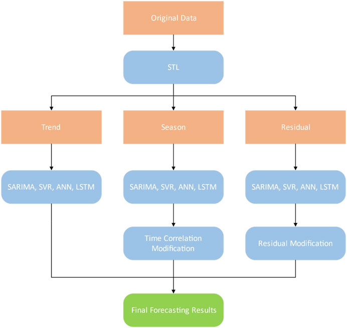
The proposed forecast framework utilizing STL decomposition, time correlation modification (embodied as annual periodicity and adjacent similarity) and residual modification is illustrated in Figure 2.

FIGURE 2

FIGURE 2. The proposed forecast framework.

In Figure 2, The proposed forecast framework consists of four steps:

In the first step, we use the Seasonal–Trend decomposition using Loess (STL decomposition) to obtain the trend, season, and residual components of the time series.

In the second step, we use SARIMA, SVR, ANN, and LSTM to forecast trend, season, and residual component, respectively.

In the third step, we use the time correlation principle to improve the forecasting accuracy of the season component. The season component presents time correlation characteristics, which embodies as annual periodicity and adjacent similarity. Here the annual periodicity means that data from the same month in the next year are similar. The adjacent similarity means that data are close to each other in adjacent months. In the second step, only adjacent similarity is used. We divide the season component into 11² subsequences, each of which represents a certain month. Then the exponential smoothing method is used to forecast each subsequence. The forecasting results are weighted with the season component predicted by each model (SARIMA, SVR, ANN, LSTM) to improve the forecasting accuracy of the season component. The weight is calculated based on the last forecasting error of the model.

In the fourth step, because the residual component has nonlinear and irregular characteristics, the individual model may only extract a certain feature of the sequence, so the forecasting accuracy is low. In fact, it is rare that a single forecasting model is always best in all cases. Each model has its own unique strengths and weaknesses. When multiple forecasting models are available, consider a combined approach, which is a good way to take full advantage of the strengths of each model. Therefore, we integrate the residual component predicted by SARIMA, SVR, ANN, and LSTM into a new sequence, and replace the residual component predicted by the above four methods with the new sequence to improve the forecasting accuracy of the residual component.

Case Study

Data Collection

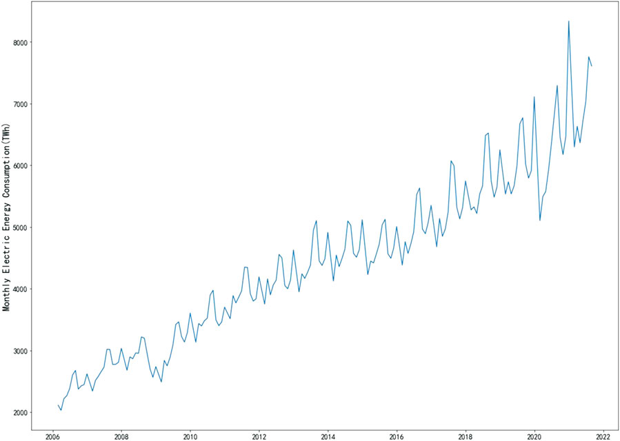
We evaluate the performance of the proposed forecasting method using the monthly electricity consumption data of China. However, these figures cannot be used directly as Chinese New Year always lasts for a few days in January or February. Almost all companies and factories have stopped operating. As a result, electricity consumption in January and February is sometimes abnormal. To avoid this problem, we treat the January and February averages as observations of a new month 1 and 2 each year, i.e., each year has 11 monthly values with a period length of 11. This study collects electricity consumption data from the beginning of 1 and 2 2006 to the end of August 2021 to keep relevant to the current situation of electricity development. These original data are shown in Figure 3.

FIGURE 3

FIGURE 3. The monthly electricity consumption of China from 1 and 2 2006 to August 2021.

Experimental Design

We select the data from 1 and 2 2006 to December 2018 as the training dataset (i.e., the first 143 data points) and the remaining data as the test dataset (i.e., the last 29 data points). The training data set is further divided into the optimization training data set and the verification data set. The optimization training data set contains the first 121 data points, and the verification training data set contains the last 22 data points. Optimization training and validation data sets were used to determine the hyperparameters of SVR, ANN, and LSTM models, while test data sets are used to evaluate forecasting performance.

Three error indices, mean absolute error (MAE), mean absolute percentage error (MAPE), and correlation coefficient (COR), are applied to evaluate the model performance according to forecast results. The official functions of the three error indices are:

$\text{MAE}=\frac{{{\displaystyle \sum }}_{i=1}^n|y_i-{\widehat{y}}_i|}{n}.$

$\text{MAPE}=\frac{100\%}{n}{\displaystyle \sum _{i=1}^n\left|\frac{y_i-{\widehat{y}}_i|}{y_i}\right|}.$

$\text{COR}=\frac{Cov\left(y_i , {\widehat{y}}_i\right)}{{\sigma }_y{\sigma }_{\widehat{y}}},$

where $y$ is the actual value, $\widehat{y}$ is the forecasted value, and $i$ is the index value of the data.

Results

Seasonal–Trend decomposition using Loess Decomposition

Figure 4 shows the STL decomposition results of the monthly electricity consumption. The trend component of the electricity consumption of China is increasing year by year, and the growth trend has accelerated since 2016. This is mainly because in 2016, eight departments in China jointly issued The Guidelines on Promoting the Substitution of Electric Energy, with a view to increasing the proportion of electric energy in the final energy consumption to 27%. Electric energy substitution is an important way to achieve carbon peak and carbon neutrality by replacing coal, oil, gas, and wood with electricity in energy consumption. The season component vibrates more and more. Due to financial crisis, extreme weather events, and epidemic, there are several relatively large negative and positive shocks on the residual component. If the original sequence is directly used, these huge shocks will seriously threaten the forecasting accuracy of the model.

FIGURE 4

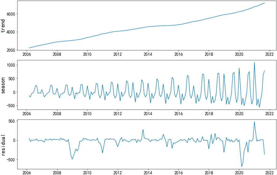
FIGURE 4. The trend, seasonal, and residual for monthly electricity consumption data decomposed by Seasonal–Trend decomposition using Loess (STL).

Table 1 shows the performance evaluation results of four models without STL decomposition and with STL decomposition. The model comparisons demonstrate that STL decomposition is effective in boosting the forecasting accuracy of monthly electricity consumption. Compared with any single model (SARIMA, SVR, ANN, LSTM), the models with STL decomposition leads to reductions in all of the evaluation indices (MAE, MAPE and COR).

TABLE 1

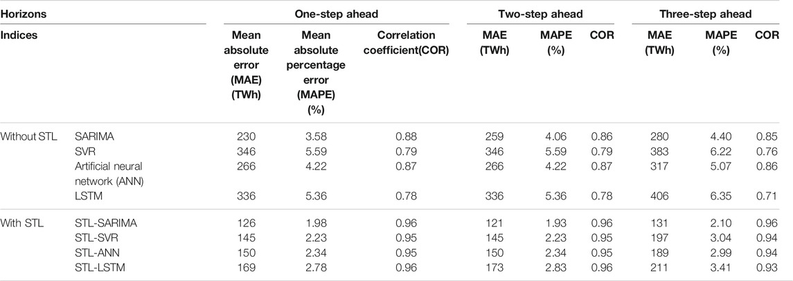
TABLE 1. Performance evaluations of different models with or without Seasonal–Trend decomposition using Loess (STL).

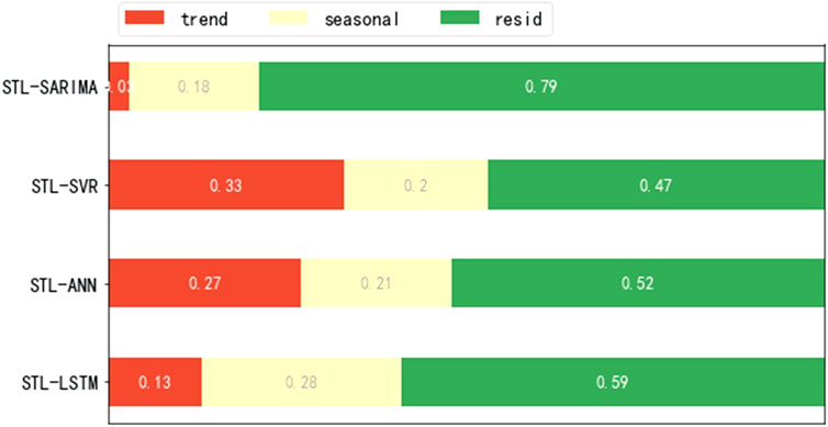
According to Table 1, the divide-and-conquer strategy improves the forecasting accuracy. Next, we analyze the source of errors, that is, the percentage of trend, season, and residual component forecasting errors to the total errors. As shown in Figure 5, for any model, most of the errors come from residual component forecast. SARIMA, in particular, was the least effective. This is because the residual component has nonlinear and irregular characteristics, and SARIMA is not good at forecasting these kinds of sequences. In addition, a single model may only extract a certain feature of the sequence, so the forecasting accuracy is low. For trend component, it can be seen that SARIMA has the highest forecasting accuracy, while for machine learning algorithms, such as SVR, ANN, and LSTM, the accuracy is not high. Therefore, it can be concluded that the traditional statistical method is better for simple sequence like trend component. The forecasting errors of season component also account for a large part.

FIGURE 5

FIGURE 5. Trend, season, random error ratio.

Time Correlation Modification

As shown in Figure 5, the errors caused by season component account for 18%–28%. In this section, we use the periodicity of the seasonal series to improve the forecasting accuracy of the season component. As we can see, the season component presents time correlation characteristics, which embodies as annual periodicity and adjacent similarity. We divide the season component into 11 subsequences, each of which represents a certain month. Then exponential smoothing method is used to forecast each subsequence. The forecasting results are weighted with the season component predicted by each model (SARIMA, SVR, ANN, and LSTM) to improve the forecasting accuracy of the season component. The weight is calculated based on the last forecast error of the model. Rows 3–6 in Table 2 show that the forecasting accuracy has been improved after time correlation modification (TCM).

TABLE 2

TABLE 2. Performance evaluations of different models with time correlation modification and residual modification.

Residual Modification

Figure 5 shows that most of the errors come from a residual component. This is because the residual component has nonlinear and irregular characteristics; a single model may only extract a certain feature of the sequence, so the forecasting accuracy of a single model is low. Therefore, we need to improve the forecasting accuracy of the residual component. We integrate the residual component predicted by SARIMA, SVR, ANN, and LSTM into a new sequence, and replace the residual component predicted by the above four methods with the new sequence to optimize each model. Rows 7–10 in Table 2 show that the forecasting accuracy has been improved after residual modification (RM).

Comparison Between Different Models

Figures 6–8 show that after STL decomposition, time correlation modification, and residual modification, the forecasting accuracy of each model has been gradually improved. Among them, the forecasting accuracy improved the most after STL decomposition. This is mainly because there are many random disturbances in the original sequence, and the model will be affected by these disturbances if it is not decomposed.

FIGURE 6

FIGURE 6. Comparison between different models for 1-month ahead forecasting.

FIGURE 7

FIGURE 7. Comparison between different models for 2-month ahead forecasting.

FIGURE 8

FIGURE 8. Comparison between different models for 3-month ahead forecasting.

Discussion

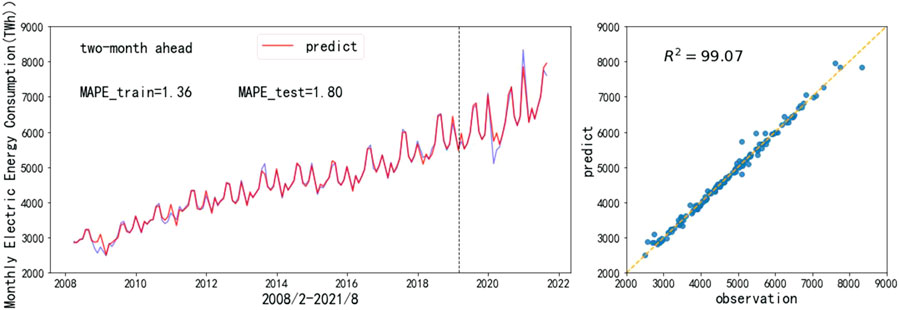
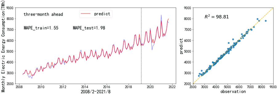
According to Figures 6–8, STL–SARIMA–TCM–RM is the most accurate forecasting model.³. As we can see, on the one hand, compared with machine learning, SARIMA is better at forecasting trend, season, and other sequences with clear patterns. That is why it is so accurate. On the other hand, SARIMA is not good at forecasting an irregular random term. Therefore, residual modification can improve the forecasting accuracy of SARIMA most significantly. Figures 9–11 show the STL–SARIMA–TCM–RM forecasting performance in the data set, as well as a scatter plot of forecasting results and actual values.

FIGURE 9

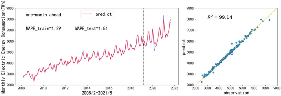
FIGURE 9. STL-SARIMA–time correlation modification (TCM)–residual modification (RM) for 1-month ahead forecasting.

FIGURE 10

FIGURE 10. STL-SARIMA-TCM-RM for 2-month ahead forecasting.

FIGURE 11

FIGURE 11. STL-SARIMA-TCM-RM for 3-month ahead forecasting.

Considering that the test set includes COVID-19, we divide the test set into 2019, 2020, and 2021. Table 3 shows that the 2019 forecast results are significantly better than that for 2020 and 2021.

TABLE 3

TABLE 3. Performance evaluation of STL-SARIMA-TCM-RM in 2019, 2020, and 2021.

Conclusion

This paper provides a novel decomposition and combination method to forecast electricity consumption. This approach first uses STL to decompose the sequence into trend, season, and residual components. Then the three decomposed subsequences are forecasted, and the season component forecasting results are modified according to the annual periodicity, and the forecasting results of the residual component of each model are integrated. The results show that STL-SARIMA-TCM-RM is the most accurate forecasting model.

In addition to electricity forecasting, we believe that the forecasting method proposed in this paper can also be used to solve other mid- and long-term forecasting problems with obvious seasonal characteristics, including tourist flow forecasting, energy consumption forecasting, traffic flow forecasting, and so on. Furthermore, this paper only focuses on univariate time series analysis and does not consider other factors affecting electricity consumption. If these factors can be introduced into the proposed learning method, the predictive performance may be better.

Data Availability Statement

The raw data supporting the conclusion of this article will be made available by the authors, without undue reservation.

Author Contributions

All authors listed have made a substantial, direct, and intellectual contribution to the work and approved it for publication.

Funding

The research was supported by National Natural Science Foundation of China (72003009).

Conflict of Interest

The authors declare that the research was conducted in the absence of any commercial or financial relationships that could be construed as a potential conflict of interest.

Publisher’s Note

All claims expressed in this article are solely those of the authors and do not necessarily represent those of their affiliated organizations, or those of the publisher, the editors and the reviewers. Any product that may be evaluated in this article, or claim that may be made by its manufacturer, is not guaranteed or endorsed by the publisher.

Footnotes

¹Wang et al., 2020.

²In the later empirical research, we treat the January and February averages as observations of a new month 1 and 2 each year.

³The STL-SARIMA-TCM-RM model is also superior to the existing models (Zhao et al., 2014; Cao and Wu, 2016; Jiang et al., 2020; Liu et al., 2020). Their models’ MAPE all above 2, and the STL-SARIMA-TCM-RM model is less than 2.

References

Akay, D., and Atak, M. (2007). Grey Prediction with Rolling Mechanism for Electricity Demand Forecasting of Turkey. Energy 32 (9), 1670–1675. doi:10.1016/j.energy.2006.11.014

CrossRef Full Text | Google Scholar

Bahrami, S., Hooshmand, R.-A., and Parastegari, M. (2014). Short Term Electric Load Forecasting by Wavelet Transform and Grey Model Improved by PSO (Particle Swarm Optimization) Algorithm. Energy 72, 434–442. doi:10.1016/j.energy.2014.05.065

CrossRef Full Text | Google Scholar

Bedi, J., and Toshniwal, D. (2019). Deep Learning Framework to Forecast Electricity Demand. Appl. Energ. 238, 1312–1326. doi:10.1016/j.apenergy.2019.01.113

CrossRef Full Text | Google Scholar

Cao, G., and Wu, L. (2016). Support Vector Regression with Fruit Fly Optimization Algorithm for Seasonal Electricity Consumption Forecasting. Energy 115, 734–745. doi:10.1016/j.energy.2016.09.065

CrossRef Full Text | Google Scholar

Cleveland, R. B., Cleveland, W., McRae, J. E., and Terpenning, I. J. (1990). STL: A Seasonal-Trend Decomposition Procedure Based on Loess (With Discussion). J. Off. Stat 6, 3–73.

Google Scholar

de Oliveira, E. M., and Cyrino Oliveira, F. L. (2018). Forecasting Mid-long Term Electric Energy Consumption through Bagging ARIMA and Exponential Smoothing Methods. Energy 144, 776–788. doi:10.1016/j.energy.2017.12.049

CrossRef Full Text | Google Scholar

Ding, S., Hipel, K. W., and DangDang, Y.-g. (2018). Forecasting China's Electricity Consumption Using a New Grey Prediction Model. Energy 149, 314–328. doi:10.1016/j.energy.2018.01.169

CrossRef Full Text | Google Scholar

Ghadimi, N., Akbarimajd, A., Shayeghi, H., and Abedinia, O. (2018). Two Stage Forecast Engine with Feature Selection Technique and Improved Meta-Heuristic Algorithm for Electricity Load Forecasting. Energy 161, 130–142. doi:10.1016/j.energy.2018.07.088

CrossRef Full Text | Google Scholar

Hamzaçebi, C., Hüseyin Avni., Es., Es, H. A., and Çakmak, R. (2019). Forecasting of Turkey's Monthly Electricity Demand by Seasonal Artificial Neural Network. Neural Comput. Applic 31 (7), 2217–2231. doi:10.1007/s00521-017-3183-5

CrossRef Full Text | Google Scholar

Hernández, D. (2013). Energy Insecurity: A Framework for Understanding Energy, the Built Environment, and Health Among Vulnerable Populations in the Context of Climate Change. Am. J. Public Health 103 (4), e32–e34. doi:10.2105/ajph.2012.301179

CrossRef Full Text | Google Scholar

Hussain, A., Rahman, M., and Memon, J. A. (2016). Forecasting Electricity Consumption in Pakistan: The Way Forward. Energy Policy 90, 73–80. doi:10.1016/j.enpol.2015.11.028

CrossRef Full Text | Google Scholar

Jiang, W., Wu, X., Gong, Y., Yu, W., and Zhong, X. (2020). Holt-Winters Smoothing Enhanced by Fruit Fly Optimization Algorithm to Forecast Monthly Electricity Consumption. Energy 193, 116779. doi:10.1016/j.energy.2019.116779

CrossRef Full Text | Google Scholar

Kandananond, K. (2011). Forecasting Electricity Demand in Thailand with an Artificial Neural Network Approach. Energies 4 (8), 1246–1257. doi:10.3390/en4081246

CrossRef Full Text | Google Scholar

Kavaklioglu, K. (2011). Modeling and Prediction of Turkey's Electricity Consumption Using Support Vector Regression. Appl. Energ. 88 (1), 368–375. doi:10.1016/j.apenergy.2010.07.021

CrossRef Full Text | Google Scholar

Kaytez, F., Taplamacioglu, M. C., Cam, E., and Hardalac, F. (2015). Forecasting Electricity Consumption: A Comparison of Regression Analysis, Neural Networks and Least Squares Support Vector Machines. Int. J. Electr. Power Energ. Syst. 67, 431–438. doi:10.1016/j.ijepes.2014.12.036

CrossRef Full Text | Google Scholar

LeCun, Y., Bengio, Y., and Hinton, G. (2015). Deep Learning. Nature 521 (7553), 436–444. doi:10.1038/nature14539

PubMed Abstract | CrossRef Full Text | Google Scholar

Lin, B., and Liu, C. (2016). Why Is Electricity Consumption Inconsistent with Economic Growth in China. Energy Policy 88, 310–316. doi:10.1016/j.enpol.2015.10.031

CrossRef Full Text | Google Scholar

Liu, Y., Wang, W., and Ghadimi, N. (2017). Electricity Load Forecasting by an Improved Forecast Engine for Building Level Consumers. Energy 139, 18–30. doi:10.1016/j.energy.2017.07.150

CrossRef Full Text | Google Scholar

Liu, Y., Zhao, J., Liu, J., Chen, Y., and Ouyang, H. (2020). Regional Midterm Electricity Demand Forecasting Based on Economic, Weather, Holiday, and Events Factors. IEEJ Trans. Elec Electron. Eng. 15, 225–234. doi:10.1002/tee.23049

CrossRef Full Text | Google Scholar

Mohamed, Z., and Bodger, P. (2005). Forecasting Electricity Consumption in New Zealand Using Economic and Demographic Variables. Energy 30 (10), 1833–1843. doi:10.1016/j.energy.2004.08.012

CrossRef Full Text | Google Scholar

Nguyen, H. T., and Nabney, I. T. (2010). Short-Term Electricity Demand and Gas Price Forecasts Using Wavelet Transforms and Adaptive Models. Energy 35 (9), 3674–3685. doi:10.1016/j.energy.2010.05.013

CrossRef Full Text | Google Scholar

Pai, P.-F., and Hong, W. C. H. (2005). Support Vector Machines with Simulated Annealing Algorithms in Electricity Load Forecasting. Energ. Convers. Manag. 46 (17), 2669–2688. doi:10.1016/j.enconman.2005.02.004

CrossRef Full Text | Google Scholar

Rendon-Sanchez, J. F., and de Menezes, L. M. (2019). Structural Combination of Seasonal Exponential Smoothing Forecasts Applied to Load Forecasting. Eur. J. Oper. Res. 275 (3), 916–924. doi:10.1016/j.ejor.2018.12.013

CrossRef Full Text | Google Scholar

Sadaei, H. J., de Lima e SilvaSilva, P. C., Guimarães, F. G., and Lee, M. H. (2019). Short-Term Load Forecasting by Using a Combined Method of Convolutional Neural Networks and Fuzzy Time Series. Energy 175, 365–377. doi:10.1016/j.energy.2019.03.081

CrossRef Full Text | Google Scholar

Sutskever, I., Vinyals, O., and QuocLe, v. (2014). Sequence to Sequence Learning with Neural Networks. Adv. Neural Inf. Process. Syst. 4 (January), 3104–3112.

Google Scholar

Zhu, L., Huang, X., Shi, H., Cai, X., and Song, Y. (2011). Transport Pathways and Potential Sources of PM10 in Beijing. Atmos. Environ. 45 (3), 594–604. doi:10.1016/j.atmosenv.2010.10.040

CrossRef Full Text | Google Scholar

Vapnik, V. (1963). Pattern Recognition Using Generalized Portrait Method. Autom. Remote Control 24, 774–780.

Google Scholar

Wang, F., Xuan, Z., Zhen, Z., Li, K., Wang, T., and Shi, M. (2020). A Day-Ahead PV Power Forecasting Method Based on LSTM-RNN Model and Time Correlation Modification under Partial Daily Pattern Prediction Framework. Energ. Convers. Manag. 212, 112766. doi:10.1016/j.enconman.2020.112766

CrossRef Full Text | Google Scholar

Wang, Y., Wang, J., Zhao, G., and Dong, Y. (2012). Application of Residual Modification Approach in Seasonal ARIMA for Electricity Demand Forecasting: A Case Study of China. Energy Policy 48, 284–294. doi:10.1016/j.enpol.2012.05.026

CrossRef Full Text | Google Scholar

Wang, Z.-X., Li, Q., Pei, L.-L., and Pei, L. L. (2018). A Seasonal GM(1,1) Model for Forecasting the Electricity Consumption of the Primary Economic Sectors. Energy 154, 522–534. doi:10.1016/j.energy.2018.04.155

CrossRef Full Text | Google Scholar

Wu, L., Gao, X., Xiao, Y., Yang, Y., and Chen, X. (2018). Using a Novel Multi-Variable Grey Model to Forecast the Electricity Consumption of Shandong Province in China. Energy 157, 327–335. doi:10.1016/j.energy.2018.05.147

CrossRef Full Text | Google Scholar

Xu, N., Dang, Y., and Gong, Y. (2017). Novel Grey Prediction Model with Nonlinear Optimized Time Response Method for Forecasting of Electricity Consumption in China. Energy 118, 473–480. doi:10.1016/j.energy.2016.10.003

CrossRef Full Text | Google Scholar

Yuan, C., Liu, S., and Fang, Z. (2016). Comparison of China's Primary Energy Consumption Forecasting by Using ARIMA (The Autoregressive Integrated Moving Average) Model and GM(1,1) Model. Energy 100, 384–390. doi:10.1016/j.energy.2016.02.001

CrossRef Full Text | Google Scholar

Zhao, H., and Guo, S. (2016). An Optimized Grey Model for Annual Power Load Forecasting. Energy 107, 272–286. doi:10.1016/j.energy.2016.04.009

CrossRef Full Text | Google Scholar

Zhao, W., Wang, J., and Lu, H. (2014). Combining Forecasts of Electricity Consumption in China with Time-Varying Weights Updated by a High-Order Markov Chain Model. Omega 45, 80–91. doi:10.1016/j.omega.2014.01.002

CrossRef Full Text | Google Scholar