Power Consumption Predicting and Anomaly Detection Based on Transformer and K-Means

With the advancement of technology and science, the power system is getting more intelligent and flexible, and the way people use electric energy in their daily lives is changing. Monitoring the condition of electrical energy loads, particularly in the early detection of aberrant loads and behaviors, is critical for power grid maintenance and power theft detection. In this paper, we combine the widely used deep learning model Transformer with the clustering approach K-means to estimate power consumption over time and detect anomalies. The Transformer model is used to forecast the following hour’s power usage, and the K-means clustering method is utilized to optimize the prediction results, finally, the anomalies is detected by comparing the predicted value and the test value. On real hourly electric energy consumption data, we test the proposed model, and the results show that our method outperforms the most commonly used LSTM time series model.

1 Introduction

Modern power systems are evolving in a more sustainable path. The load demand for domestic electrical energy is gradually increasing as the number of household appliances and electric cars increases. Statistics show that residences and commercial buildings account for three-fifths of global electricity use (Desai, 2017). The power system has grown in complexity and intelligence, and more modern information transmission technology has been implemented, making grid processing more convenient and secure (Bayindir et al., 2016). Moreover, electric energy consumption in everyday living is also difficult and variable. Electric energy usage, for example, may vary significantly depending on the season, and consumption on working days and working days will fluctuate. At the same time, there will be anomalies in the electrical load, such as forgetting to turn off electrical appliances, failure of electrical appliances and even the theft of electricity, and so on, resulting in a much larger electrical demand than typical. As a result, detecting unusual consumption data is critical.

Abnormal detection can enhance abnormal electric energy consumption to achieve energy savings, remind users to discover malfunctioning electrical appliances or modify bad electricity usage patterns, lower users’ energy consumption expenses, and promote electricity consumption safety awareness. The most crucial factor is that you can locate the source of the power theft (McLaughlin et al., 2009). According to the survey, power theft accounts for about half of the energy lost in some developing countries (Antmann,2009), and anomaly detection technologies can successfully combat this scenario.

Anomaly detection, as the name suggests, is the method of recognizing data that differs from the usual. Anomalies in data are situations that do not follow the specified usual behavior pattern (Chandola et al., 2009). Anomalies are classified into three types: point anomalies, aggregate anomalies, and context anomalies. A point anomaly occurs when one point in the data is excessively high or too low in comparison to other points. The anomalous phenomena of a group of data compared to the full data set is referred to as a collection anomaly, and it only happens in the data set with the correlation between the data. Contextual abnormality refers to the abnormality when the data is combined with the context in the data set (Chandola et al., 2009). In this paper, abnormal power consumption means that if the difference between the power consumption predicted by the model and the real power consumption in a certain hour is greater than the threshold we set through the experiment, the current hour power consumption is considered abnormal, so the main task of this paper is to detect point anomalies.

Because the characteristics of variables are various, traditional models primarily focus on univariate prediction and anomaly detection (Hu et al., 2018). Univariate models are typically utilized in cases where there are too many other features or when vectorization is difficult, such as stock prediction (Hsieh et al., 2011). Various industries, such as speech recognition (Graves et al., 2013) and NLP (Natural Language Processing) (Nadkarni et al., 2011), have adopted deep learning technology and achieved remarkable success as a result of the rapid development of the field of deep learning. Time series analysis (Kuremoto et al., 2014), of course, has also a significant advancement. Traditional statistical methods such as ARIMA (Auto-Regressive Integrated Moving Average) (Yuan et al., 2016) and SARIMA (Seasonal ARIMA) (Ahn et al., 2015) were defeated by the proposed LSTM (Long and Short-Term Memory network) (Hochreiter and Schmidhuber,1997). For energy consumption prediction and anomaly detection, a lot of work on LSTM has been done.

However, with the introduction of Google’s Transformer model (Vaswani et al., 2017), this model was first successfully used to the field of machine translation, and then it spread to other significant fields such as speech recognition (Wang et al., 2020), and so on. Since machine translation technology involves the processing of time series, we seem to be able to use the Transformer model for time series forecasting tasks. Transformer uses self-attention and multi-head self-attention for semantic extraction. When it comes to the long-distance dependence of features in time series, self-attention can naturally solve this problem, because there are connections between all features of time series when integrating features, and the relative position information between the input time series features is preserved through sinusoidal position encoding. It is not like RNN (Recurrent Neural Network) that needs to be gradually passed to the back through hidden layer node sequences, nor is it like CNN (Convolutional Neural Networks) that needs to be captured long distance features by increasing the network depth, Transformer has some advantages in processing time series features.

As a result, in this paper, we propose a new power consumption prediction and anomaly detection model that combines deep learning and clustering methods. The following are the contributions:

1) For time series prediction of power consumption, we merged the current popular Transformer deep learning model with K-means clustering. We reasoned that the historical time data contributes differentially to the expected value due to the regular behavior of household users. The K-means method can be used to locate data clusters that contribute more to the projected value, allowing the Transformer model prediction value to be optimized further.

2) In the experiment, we employed multi-dimensional data. The data dimension also incorporates auxiliary information data such as voltage, current, and the power consumption of various household appliances, in addition to the fundamental power consumption.

3) We compared the proposed method to the LSTM and only Transformer model’s prediction performance. Experiments have revealed that the proposed combination method’s error between predicted and true values is lower than those of LSTM and single Transformer.

4) To demonstrate the proposed method’s superior performance in anomaly detection, we manually added anomalous data into the test data and treated it as a true anomaly.

The following is how we organize this paper. We introduce relevant research on power consumption and anomaly detection in Section 2. The data set used in the experiment, as well as the data set’s preparation approach, are shown in Section 3. We describe our model’s implementation approach and procedure in detail in Section 4. We compare the performance of model prediction and anomaly detection with different models in Section 5. This paper was summarized in the last section.

2 Related Works

Researchers have done a lot of research since power consumption prediction and anomaly detection are so crucial in the power energy system. Box et al. (2015) developed time series forecasting approaches like as Auto-Regressive (AR), ARIMA (Auto-Regressive Integrated Moving Average), and SARIMA (Seasonal ARIMA) in the economic sphere, and they had good results. To predict the value at a specific moment in the time series, the AR model primarily uses the weighting of all values preceding that time. ARIMA primarily employs the point before to the time to add a random vector in order to forecast the value at that time. SARIMA is mostly used for time series data with obvious seasonal differences. Ouyang et al. (2019b) improved the performance of wind power ramp prediction by combining the advantages of AR models and Markov chain. To detect anomalies, Yan et al. (2014) integrated the AR approach with SVM (Support Vector Machine) Ma and Guo (2014). ARIMA was used by Ediger and Akar (2007) to forecast fuel energy use in Turkey. The time series of ARIMA power consumption was utilized by Alberg and Last (2018) to estimate future power consumption, and Krishna et al. (2015) employed ARIMA for half-hour granular power consumption data. SARIMA was applied by Ahn et al. (2015) for long-term and mid-term load forecasting. The unsupervised K-means approach Münz et al. (2007) groups the data to identify anomalies that are outside of the cluster. Simultaneously, the autoencoder model has been a huge success. The data is analyzed using unsupervised methods. The difference between input and output is utilized to detect whether the data is aberrant, from compression and abstraction to recovery and rebuilding. For anomaly detection, Al-Abassi et al. (2020) presented unsupervised stacked autoencoders for smart cyber-physical grids. Deb et al. (2015) developed an artificial neural network for predicting building energy usage in Singapore, and it was shown to be accurate.

The advancement of deep learning has improved the accuracy and performance of large data processing and prediction. Deep learning was used extensively in wind speed prediction (Khodayar et al., 2017), stock prediction (Rather et al., 2015), automated Vehicles (Shen et al., 2020) and other researches, and power grid technology has also incorporated the nerve of deep learning. The network is used to forecast and detect how much energy the user consumes. Ouyang et al. (2019a) proposed the use of Deep Belief Network (DBN) to predict hourly power load. According to Shi et al. (2017), predicting the electricity usage of a single customer in Ireland is the same as using a deep recursive network. For time series, LSTM can forecast and detect anomalies (Malhotra et al., 2016; Siami-Namini et al., 2018). Wang et al. (2019) proposed combining seasonal features with LSTM for power load forecasting and anomaly detection. However, because ARIMA requires time series data to be stationary and it can only capture linear relationships, but not non-linear relationships. For the LSTM model, its output at the current time requires not only the input at the current time, but also the output at the previous time. This makes the LSTM model unable to parallelize operations, resulting in too long training time when processing time series features. On the other hand, the Transformer model has had a lot of success in the field of speech recognition and natural language processing since it was introduced. As a result, we propose in this paper that we utilize the transformer model to estimate electric energy load, then apply the k-means approach to further improve the prediction results, and then compare the prediction results to the test data to look for anomalies.

3 Datasets

For the experiment, we used hour-level electricity load data from a French family for 1,440 days (2006-12-17 to 2010-11-25). We selected 3 h of data for display, as shown in Table 1, except for “global_active_power” represents the total active power consumed by the household, and other data includes “global_reactive_power” representing the total reactive power consumed by the household, “voltage” representing the average voltage per hour, “global_intensity” representing the average current intensity, “sub_metering_1” representing the active electrical energy of the kitchen, “sub_metering_2” representing the active energy of the laundry, “sub_metering_3” representing the active energy of the climate control system, “sub_metering_4” representing other active energy. The hourly power load change diagram for 3 days which are all weekdays is shown in Figure 1. It can be seen that power consumption has increased significantly in the morning, noon and evening, and electricity consumption conforms to the law of electricity consumption in French households during workdays. To make the data more stable, we apply the Min-Max Normalization procedure. This will make the model’s training easier and its convergence faster. We designed the model supervision task to estimate the following hour’s electric energy usage based on multivariate data collected every 23 h, and we implemented it by using a 23-hour sliding window.

TABLE 1

TABLE 1. Sample display of the data set used in this paper.

FIGURE 1

FIGURE 1. Hourly household electric energy consumption change diagram for 3 consecutive days.

4 Methodology

We partitioned the data into 24-hour groups using a sliding window, then trained k-means clustering for the first 23 h of each group of real test data into k clusters, while also used the 23-hour real load data training Transformer model predicts the next hour’s load data, then through the trained K-means to get the appropriate centroid as the final prediction result. Figure 2 depicts the framework of our model.

FIGURE 2

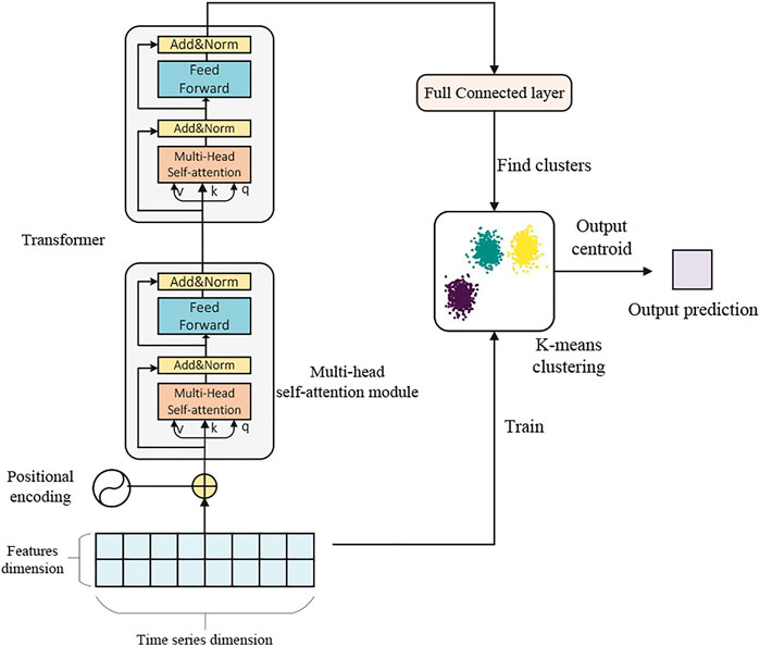
FIGURE 2. The main framework of our model.

4.1 Transformer Model

Initial and foremost, Positional Encoding is the first phase in the Transformer model utilized in this essay. Because Transformer does not have a cyclic structure like LSTM, it presents a new positional encoding strategy to capture the input time series information, as indicated in Eqs 1, 2. The basic idea is to add sine and cosine functions of various frequencies as position codes to the normalized input sequence, allowing the Transformer model’s multi-head attention mechanism to fully capture time series data with more dimensions.

$P{E}_{(pos,2i)}=\sin (pos/10000^{2i/d_{model}})(1)$

$P{E}_{(pos,2i+1)}=\cos (pos/10000^{2i/d_{model}}),i\in [0,\dots ,d_{model}/2)(2)$

where pos is the vector position of each time. For example, in the time series data in this paper, the pos of the first hour of each group is 0, and the pos of the second hour is 1, 2i and 2i + 1 respectively represent the even position and the odd position. d_model represents the length of the feature vector per hour. Next, we use X = [x₁, x₂, …, x_n] to represent the input sequence combined with position encoding, and pass the multi-head self-attention of the Transformer model:

$MultiHead(Q,K,V)=Concat(hea{d}_1,\dots ,hea{d}_i)W^o(3)$

$hea{d}_i=Attention(Q{W}_i^Q,K{W}_i^K,V{W}_i^V)(4)$

In the above formula, $Q=q_1{w}^{q_1},K=k_1{w}^{k_1},V=v_1{w}^{v_1}$, q₁ = k₁ = v₁ = X. In the Transformer model, the Attention module first undergoes a linear transformation of Q (Query), K (Key), and V (Value). Each time Q, K, and V perform the linear transformation, the parameter W is different, and then input to Scaling dot product attention, the formula is as (5), note that it is necessary to do i times here, in fact, it is the so-called multi-head, and each time counts as one head. Then concatenate the attention results of the i times of scaling dot product, and then perform a linear transformation to obtain the value as the result of the multi-head attention. The advantage of this is that it allows the model to learn relevant information in different representation subspaces. The calculation of the Attention module uses Scaled Dot-product:

$Attention(Q,K,V)=softmax\left(\frac{Q{K}^T}{\sqrt{d_k}}\right)V(5)$

where d_k is the last dimension of the shape of Q, K, V, divided by $\sqrt{d_k}$ to prevent d_k from being too large and the softmax function’s gradient becoming too tiny when QK^T is too large. The residual connection structure is then used to narrow the network’s attention to solely the differences. In multi-layer network structures, it is frequently used:

$L=LayerNorm(X+MultiHead(Q,K,V))(6)$

where LayerNorm is Layer Normalization, which normalizes each neuron and adjusts the mean and variance of the input data to be the same, which will speed up the convergence. Then input L into the FeedForward layer, which is composed of two fully connected layers, the first layer uses the Relu activation function, and the second layer does not use the activation function:

$s=\max (0,L{W}_1+b_1)W_2+b_2(7)$

Similarly, use residual connection and Layer Normalization again to get the output S_E:

$S_E=LayerNorm(L+s)(8)$

Our experiment uses a 2-layer Transformer multi-head attention module, which means that the output S_E needs to be re-input to the structure output S_E2 described above. Finally, the output will be decoded and dimensionality reduction operations through the fully connected layer:

$K=W_3{S}_{E2}(9)$

4.2 K-Means Clustering Method

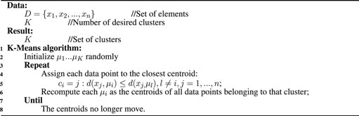
Clustering is the division of a sample set into several disjoint subsets (sample clusters), which is a typical unsupervised machine learning algorithm. When using clustering to classify samples, Euclidean Distance is used as the measurement criterion of sample similarity. The higher the similarity, the smaller the Euclidean Distance of the sample. K-means clustering is a well-known algorithm among clustering algorithms. It needs to determine the number of clusters k first when clustering, and k is given by the user. Each cluster passes through its centroid (the mean value of all elements in the cluster). The workflow of k-means is also very simple. First, randomly select k initial points as the initial centroids of each cluster, and then assign each point in the data set to the cluster closest to it. The distance calculation uses the Euclidean Distance mentioned above. The algorithm of k-means is shown in Algorithm 1:

Algorithm 1 K-means algorithm.

4.3 Model Development

First, we divide the data set into a training set and a test set. Since the data set contains a total of 1,440 days of hourly data, we choose 1,240 days of data as the training set and 200 days of data as the test set. For the Transformer model, we choose two consecutive layers of multi-head self-attention modules, and each multi-head attention is set to 4 attention heads. The input data shape is 23 time steps and 8 features. For K-means clustering, we experimented with k = 2, 5, 8, 10, 11, and 15 respectively, and finally selected the cluster with k = 10. We choose the mean-square error of the predicted data and the original data, that is, MSE (Mean-Square Error) as the loss function, and Adam as the optimizer of the model. And set the epoch of the training model to 300, and the batch size to 200.

4.4 Model Prediction and Evaluation

We believed that the nearest neighbor of the real training data has the most impact on the forecast value, thus in the first 23 h of each group, we trained k-means clustering, partitioned the data into k categories, and provided the load K predicted by the Transformer model for the next hour as the final prediction output, then found the centroid in the trained K-means cluster. We analyzed the model’s prediction ability by fitting the predicted value to the test value and calculating the RMSE (Root Mean Squard Error) of the forecasted value and the test value to measure the prediction’s accuracy, and we compared it to the commonly used LSTM model.

4.5 Anomaly Detection

Because the model calculates the anticipated value based on a huge quantity of historical data, the forecasted values will generally follow the data’s trend. If the test value differs significantly from the projected value, it indicates that the test value has deviated too far from the data trend and may be abnormal. The score between the predicted value and the test value obtained after the Transformer model and k-means clustering is calculated in this research. The formula can be found in Eq. 10. In order to better analyze the difference, we normalized the score, the formula is as Eq. 11. The value of score collected from several experiments was used to determine a threshold. When the score between the predicted value and the test value exceeds the threshold, the test value is considered abnormal. The experiment can also evaluate whether the user is prone to having electricity theft by setting a time series window and a threshold for the number of anomalies. If the number of abnormalities in the time series data in a window is greater than the threshold, it means that the time series data are abnormal, and the user may have the suspicion of steal electricity. To better compare the accuracy of anomaly detection, we manually insert abnormal data points in the test data and compare our model with K-means and LSTM.

$scor{e}_t=\frac{|predicte{d}_t-tes{t}_t|}{av{g}_{i\in T}(|predicte{d}_i-tes{t}_i|)}(10)$

$\widetilde{scor{e}_t}=\frac{scor{e}_t-\min (score)}{\max (score)-min(score)}(11)$

5 Experiment Results

5.1 Consumption Prediction

We opted to compare the model against the most popular LSTM model for time series data prediction in order to test its performance. The LSTM is a variant of the recurrent neural network RNN. It is a unique RNN that incorporates three different types of gating to address the problem of gradient disappearance and explosion during lengthy sequence training. Simply put, LSTM outperforms standard RNNs in longer sequences, making it ideal for time series forecasting jobs.

Figure 3 shows how the training and test loss of the Transform model used in this paper changes at 300 epoch. It can be observed that the model converges quickly, and the figure shows that there is no overfitting in the model. All of this is achievable because of the Transformer model’s benefits in time series processing.

FIGURE 3

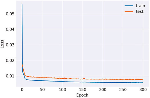
FIGURE 3. Train and test loss over the 300 epochs of our model.

Figure 4 depicts the test set’s real-time power consumption data over 3 days, as well as a comparison of our model’s and the LSTM model’s prediction results on the test set. The blue line represents the actual data, the red line represents our model’s predicted value, the green line represents the LSTM model’s predicted value, and the purple line indicates the lone Transformer’s predicted value. Our model’s forecast data is more in accordance with the real test data, as can be shown. The RMSE of the model, on the other hand, are used to assess the model’s fit. Our model has an RMSE of 0.73, the Transformer has an RMSE of 0.77, and the LSTM has an RMSE of 0.86. In terms of prediction accuracy, our model outperforms LSTM by 15%, while Transformer outperforms LSTM by just 10%. After our analysis, because the dimensionality of the feature vector of each time series in our time series data is too small, which leads to the failure of the full performance of the Transformer model.

FIGURE 4

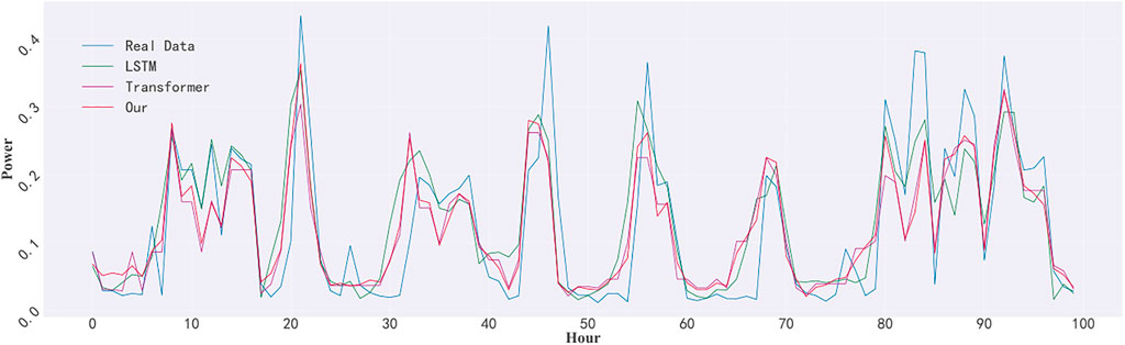
FIGURE 4. Comparison of our model and LSTM predicted value fitting real data.

5.2 Anomaly Detection

After a lot of testing and tweaking, we ultimately settled on 0.45 as the threshold. This means that any point with a score higher than 0.45 will be considered anomalous. The change in score data over 2,500 h is presented in Figure 5, with the red dashed line representing the threshold and the purple point representing the abnormal point. The data scores are primarily focused between 0 and 0.3, and there are relatively few aberrant spots, as can be shown. In practical applications, we can adjust the threshold size based on the scene being used, and lower or increase the threshold size based on the strictness of anomaly detection, a lower threshold is more stringent, allowing for the detection of more anomalies, on the other hand, a higher threshold is more tolerant, allowing for the detection of fewer anomalies.

FIGURE 5

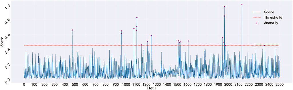
FIGURE 5. Scores and anomalies exceeding the threshold for 2,500 h.

We utilized the strategy of randomly inserting abnormal points in the test data to better compare and assess the model’s anomaly detection capabilities because this experimental data set does not mark aberrant time points. In the 200 days (4,800 h) of the test set, we randomly selected a value every day and double it, and assume it is an outlier, so there are 200 outliers in the 4,800 data in the test set. For comparison, we separately used the clustering method K-means and the most popular depth method LSTM to detect abnormal points. Using the K-means approach, we discovered a total of 68 abnormal points, of which only 56 were the abnormal points we manually inserted into the data set. Using the LSTM model, we retrieved a total of 162 anomalies, 120 of which were the anomaly points we manually inserted into the data set. Our combined Transformer and K-means model found 165 anomalies, 132 of which were the abnormal points we manually added to the data set. The accuracy, precision, recall, and F1 of the three models are shown in Table 2. The predicted RMSE of LSTM and our model are also shown in the table.

TABLE 2

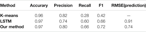
TABLE 2. Comparison with some methods.

6 Conclusion

The prediction of electric energy consumption and the identification of anomalies are critical in the functioning of the power grid, and the processing of multi-variable time series is a difficult challenge. We present a model that combines Transformer and K-means approaches in this article. Every 23 h of training data is separated into k clusters using K-means clustering. At the same time, this training data are used to train the Transformer model to predict the following hour’s power usage, with the predicted value being placed into the trained K-means cluster and the cluster’s centroid serving as the final predicted value. Finally, look for anomalies by comparing the anticipated value to the actual test results. The experimental results prove that the model achieves prediction accuracy with less error and high anomaly detection performance. In the future, we’ll strive to improve prediction and anomaly detection accuracy, as well as study the differences between power consumption prediction and anomaly detection in different seasons, environments, and other scenarios, and other issues that need to be addressed.

Data Availability Statement

The datasets presented in this study can be found in online repositories. The names of the repository/repositories and accession number(s) can be found below: https://archive.ics.uci.edu/ml/datasets/individual+household+electric+power+consumption.

Author Contributions

JZ: conceptualization, methodology, data preprocessing, and writing-original draft preparation. HZ: visualization, investigation. SD: experimental training and testing. XZ: supervision and reviewing.

Funding

This work was supported in part by the National Natural Science Foundation of China under Grants 71901215, 71901191, the National University of Defense Technology Research Project ZK20-46, and the Outstanding Youth Talents Program of National University of Defense Technology.

Conflict of Interest

The authors declare that the research was conducted in the absence of any commercial or financial relationships that could be construed as a potential conflict of interest.

Publisher’s Note

All claims expressed in this article are solely those of the authors and do not necessarily represent those of their affiliated organizations, or those of the publisher, the editors and the reviewers. Any product that may be evaluated in this article, or claim that may be made by its manufacturer, is not guaranteed or endorsed by the publisher.

References

Ahn, B.-H., Choi, H.-R., and Lee, H.-C. (2015). Regional Long-Term/mid-Term Load Forecasting Using Sarima in south korea. J. Korea Academia-Industrial cooperation Soc. 16, 8576–8584. doi:10.5762/kais.2015.16.12.8576

CrossRef Full Text | Google Scholar

Al-Abassi, A., Sakhnini, J., and Karimipour, H. (2020). “Unsupervised Stacked Autoencoders for Anomaly Detection on Smart Cyber-Physical Grids,” in 2020 IEEE International Conference on Systems, Man, and Cybernetics (SMC) (IEEE), 3123–3129. doi:10.1109/smc42975.2020.9283064

CrossRef Full Text | Google Scholar

Alberg, D., and Last, M. (2018). Short-term Load Forecasting in Smart Meters with Sliding Window-Based Arima Algorithms. Vietnam J. Comput. Sci. 5, 241–249. doi:10.1007/s40595-018-0119-7

CrossRef Full Text | Google Scholar

Antmann, P. (2009). Reducing Technical and Non-technical Losses in the Power Sector.

Google Scholar

Bayindir, R., Colak, I., Fulli, G., and Demirtas, K. (2016). Smart Grid Technologies and Applications. Renew. Sustain. Energ. Rev. 66, 499–516. doi:10.1016/j.rser.2016.08.002

CrossRef Full Text | Google Scholar

Box, G., Jenkins, G. M., Reinsel, G. C., and Ljung, G. M. (20152015). Time Series Analysis: Forecasting and Control.

Google Scholar

Chandola, V., Banerjee, A., and Kumar, V. (2009). Anomaly Detection. ACM Comput. Surv. 41, 1–58. doi:10.1145/1541880.1541882

CrossRef Full Text | Google Scholar

Deb, C., Eang, L. S., Yang, J., and Santamouris, M. (2015). Forecasting Energy Consumption of Institutional Buildings in singapore. Proced. Eng. 121, 1734–1740. doi:10.1016/j.proeng.2015.09.144

CrossRef Full Text | Google Scholar

Desai, B. H. (2017). 14. United Nations Environment Program (Unep). Yearb. Int. Environ. L. 28, 498–505. doi:10.1093/yiel/yvy072

CrossRef Full Text | Google Scholar

Ediger, V. Ş., and Akar, S. (2007). Arima Forecasting of Primary Energy Demand by Fuel in turkey. Energy policy 35, 1701–1708. doi:10.1016/j.enpol.2006.05.009

CrossRef Full Text | Google Scholar

Graves, A., Mohamed, A.-r., and Hinton, G. (20132013). IEEE International Conference on Acoustics, Speech and Signal Processing. IEEE, 6645–6649. doi:10.1109/icassp.2013.6638947Speech Recognition with Deep Recurrent Neural Networks

CrossRef Full Text | Google Scholar

Hochreiter, S., and Schmidhuber, J. (1997). Long Short-Term Memory. Neural Comput. 9, 1735–1780. doi:10.1162/neco.1997.9.8.1735

PubMed Abstract | CrossRef Full Text | Google Scholar

Hsieh, T.-J., Hsiao, H.-F., and Yeh, W.-C. (2011). Forecasting Stock Markets Using Wavelet Transforms and Recurrent Neural Networks: An Integrated System Based on Artificial Bee colony Algorithm. Appl. soft Comput. 11, 2510–2525. doi:10.1016/j.asoc.2010.09.007

CrossRef Full Text | Google Scholar

Hu, M., Ji, Z., Yan, K., Guo, Y., Feng, X., Gong, J., et al. (2018). Detecting Anomalies in Time Series Data via a Meta-Feature Based Approach. Ieee Access 6, 27760–27776. doi:10.1109/access.2018.2840086

CrossRef Full Text | Google Scholar

Khodayar, M., Kaynak, O., and Khodayar, M. E. (2017). Rough Deep Neural Architecture for Short-Term Wind Speed Forecasting. IEEE Trans. Ind. Inf. 13, 2770–2779. doi:10.1109/tii.2017.2730846

CrossRef Full Text | Google Scholar

Krishna, V. B., Iyer, R. K., and Sanders, W. H. (2015). “Arima-based Modeling and Validation of Consumption Readings in Power Grids,” in International Conference on Critical Information Infrastructures Security (Springer), 199–210.

Google Scholar

Kuremoto, T., Kimura, S., Kobayashi, K., and Obayashi, M. (2014). Time Series Forecasting Using a Deep Belief Network with Restricted Boltzmann Machines. Neurocomputing 137, 47–56. doi:10.1016/j.neucom.2013.03.047

CrossRef Full Text | Google Scholar

Ma, Y., and Guo, G. (2014). Support Vector Machines Applications, Vol. 649. Springer.

Google Scholar

Malhotra, P., Ramakrishnan, A., Anand, G., Vig, L., Agarwal, P., and Shroff, G. (2016). Lstm-based Encoder-Decoder for Multi-Sensor Anomaly Detection. arXiv preprint arXiv:1607.00148.

Google Scholar

McLaughlin, S., Podkuiko, D., and McDaniel, P. (2009). “Energy Theft in the Advanced Metering Infrastructure,” in International Workshop on Critical Information Infrastructures Security (Springer), 176–187.

Google Scholar

Münz, G., Li, S., and Carle, G. (2007). “Traffic Anomaly Detection Using K-Means Clustering,” in GI/ITG Workshop MMBnet, 13–14.

Google Scholar

Nadkarni, P. M., Ohno-Machado, L., and Chapman, W. W. (2011). Natural Language Processing: an Introduction. J. Am. Med. Inform. Assoc. 18, 544–551. doi:10.1136/amiajnl-2011-000464

CrossRef Full Text | Google Scholar

Ouyang, T., He, Y., Li, H., Sun, Z., and Baek, S. (2019a). Modeling and Forecasting Short-Term Power Load with Copula Model and Deep Belief Network. IEEE Trans. Emerg. Top. Comput. Intell. 3, 127–136. doi:10.1109/tetci.2018.2880511

CrossRef Full Text | Google Scholar

Ouyang, T., Zha, X., Qin, L., He, Y., and Tang, Z. (2019b). Prediction of Wind Power Ramp Events Based on Residual Correction. Renew. Energ. 136, 781–792. doi:10.1016/j.renene.2019.01.049

CrossRef Full Text | Google Scholar

Rather, A. M., Agarwal, A., and Sastry, V. N. (2015). Recurrent Neural Network and a Hybrid Model for Prediction of Stock Returns. Expert Syst. Appl. 42, 3234–3241. doi:10.1016/j.eswa.2014.12.003

CrossRef Full Text | Google Scholar

Shen, X., Zhang, X., Ouyang, T., Li, Y., and Raksincharoensak, P. (2020). Cooperative Comfortable-Driving at Signalized Intersections for Connected and Automated Vehicles. IEEE Robot. Autom. Lett. 5, 6247–6254. doi:10.1109/lra.2020.3014010

CrossRef Full Text | Google Scholar

Shi, H., Xu, M., and Li, R. (2017). Deep Learning for Household Load Forecasting a Novel Pooling Deep Rnn. IEEE Trans. Smart Grid 9, 5271–5280.

Google Scholar

Siami-Namini, S., Tavakoli, N., and Namin, A. S. (2018). “A Comparison of Arima and Lstm in Forecasting Time Series,” in 2018 17th IEEE International Conference on Machine Learning and Applications (ICMLA) (IEEE), 1394–1401. doi:10.1109/icmla.2018.00227

CrossRef Full Text | Google Scholar

Vaswani, A., Shazeer, N., Parmar, N., Uszkoreit, J., Jones, L., Gomez, A. N., et al. (2017). Attention Is All You Need. Advances in Neural Information Processing Systems, 5998–6008.

Google Scholar

Wang, X., Zhao, T., Liu, H., and He, R. (20192019). “Power Consumption Predicting and Anomaly Detection Based on Long Short-Term Memory Neural Network,” in IEEE 4th international conference on cloud computing and big data analysis (ICCCBDA) (IEEE), 487–491. doi:10.1109/icccbda.2019.8725704

CrossRef Full Text | Google Scholar

Wang, Y., Mohamed, A., Le, D., Liu, C., Xiao, A., Mahadeokar, J., et al. (2020). “Transformer-based Acoustic Modeling for Hybrid Speech Recognition,” in ICASSP 2020-2020 IEEE International Conference on Acoustics, Speech and Signal Processing (ICASSP) (IEEE), 6874–6878. doi:10.1109/icassp40776.2020.9054345

CrossRef Full Text | Google Scholar

Yan, K., Shen, W., Mulumba, T., and Afshari, A. (2014). Arx Model Based Fault Detection and Diagnosis for Chillers Using Support Vector Machines. Energy and Buildings 81, 287–295. doi:10.1016/j.enbuild.2014.05.049

CrossRef Full Text | Google Scholar

Yuan, C., Liu, S., and Fang, Z. (2016). Comparison of China's Primary Energy Consumption Forecasting by Using ARIMA (The Autoregressive Integrated Moving Average) Model and GM(1,1) Model. Energy 100, 384–390. doi:10.1016/j.energy.2016.02.001

CrossRef Full Text | Google Scholar