Simulation Study on the Development Process and Phase Interface Structure of Gas-Liquid Slug Flow in a Horizontal Pipe

Here, a unified 3D numerical model of gas-liquid two-phase flow in a horizontal pipe was established using the interface capture method based on the open source software package OpenFOAM. Through numerical simulation of the natural slugging and development process of slug flow under different working conditions, the motion, phase interface structure, pressure and velocity field distributions of the liquid slug were fully developed and analyzed. The simulation results are consistent with the experiment. The results showed that during the movement of the slug head, there is a throwing phenomenon and a wave-like motion of the liquid slug. In addition, the slug tail and body area have very similar velocity profiles, and the overall velocity field distribution becomes more uniform with the development of liquid slug. Moreover, there are sudden pressure fluctuations at the head and tail of the liquid slug.

Introduction

The mixed transmission pipelines on the seabed laid along the seabed terrain are mainly horizontal and near horizontal. Slug flow is the most common flow pattern in the mixed transmission of oil and gas in horizontal and near horizontal pipelines, and the production parameters of most oil wells are within the parameter range of this flow pattern (Bonizzi, 2003). Due to the randomness, complexity and intermittence of slug flow, the understanding of its flow characteristics and phase interface structure is not thorough. The fluctuation of pressure and flow caused by slug flow has an important impact on deep-sea oilfield and the design of production equipment. In the beginning macroscopic studies are focused on average length and holding capacity of liquid slugs, but now researchers have gradually turned to the more complex study of the natural development process and transient gas-liquid interface structures of liquid slugs.

Taitel’s study (Taitel et al., 2000) showed that the steady-state model often presents non-physics profiles when calculating the slug flow in a downcast pipe. According to the characteristics of gas-liquid distribution and pressure drop fluctuation, Yin et al. (2022) divided intermittent flow and segregated flow into various sub-flow patterns. The distribution of the flow patterns was summarized under different working conditions. The experimental results enhance the understanding of the morphology and evolution process of gas-liquid flow. Ishii (Ishii, 2006) established a 1D two-fluid model, but the governing and constitutive equations of different flow patterns were quite different. Lu (2015) used six commercial finite volume codes to simulate the slug flow in horizontal pipe sections by 1D two-fluid model, and compared the results with experimental data, finding that the simulated slug flow characteristics were quite different from the experimental ones. Ekambara et al. (2008) used the VOF (volume of fluid) model to simulate the internal phase distribution of the slug flow in a horizontal pipeline with an inner diameter of 50.3 mm. The results indicated that the volume fraction had a maximum near the upper pipe wall, and the profiles tended to flatten with increasing liquid flow rate. It was found that increasing the gas flow rate at fixed liquid flow rate would increase the local volume fraction. Abdulkadir et al. (2013) used VOF model and RANS (Reynolds-averaged Navier-Stokes) turbulence model to simulate the air silicone oil slug flow in 90°vertical elbow and compared it with the experimental results. It was found that the flow pattern before and after turning was consistent with the one captured by high-speed camera, and the model could predict the gas phase distribution at turning. Glatzel et al. (2008) used VOF model to simulate the liquid-liquid and gas-liquid two-phase flow in T-shaped microchannel, and analyzed the bubble shape in gas-liquid two-phase flow, micro droplet volume and separation time in liquid-liquid two-phase flow. There was a gap between the simulated phase interface structure and the experimental results. Ratkovich et al. (2009) established a 2D vertical pipe model with inner diameter of 190.5 mm and length of 3.4 m by using VOF model to analyze the void fraction of gas-liquid two-phase slug flow of Newtonian fluid and non-Newtonian fluid. The simulation results of void fraction were in good agreement with the experimental results. Deendarlianto et al. (2016) used VOF model to simulate gas-liquid two-phase flow in horizontal pipe. The results showed that there was a quantitative consistency between the calculated results and the experimental data for the changes of long bubble length and liquid holdup. A slug tracking model was proposed by Zheng et al. (1994), although it was found that this model cannot fundamentally simulate the natural evolution process of the slug, and the resulting calculations of high gas-liquid velocity are yet to be verified. Vallée et al. (2008), Vallée et al. (2010) used CFX software in conjunction with the Euler two-phase flow and SST Turbulence models to establish a 2D numerical model of slug flow; however, due to the restriction of inlet conditions in the model, the gas-liquid interface structure of the slug flow was quite different from that observed in experiments. Ramdin and Henkes (2011), Ramdin and Henkes (2012) established 2D and 3D models using FLUENT software. They simulated Benjamin bubbles in a horizontal tube and Taylor bubbles in a vertical tube and analyzed the influence of viscosity and surface tension on the bubbles. For the most part, the simulation results were consistent with the experimental results; however, when the surface tension was high, the 2D Benjamin bubble model greatly deviated from the experimental results. De Schepper et al. (2008) used VOF model and piecewise linear interface calculation (PLIC) interface recombination method to build a 3D horizontal pipe model. The simulation results for the air-water two-phase flow pattern at different gas-liquid velocities were consistent with the baker flow pattern, but the gas-liquid interface structures of each flow pattern were quite different from experiments.

From the aforementioned studies, it is found that the idea of establishing these transient models is to divide the slug flow into liquid slug region and bubble slug region, and simulate the transient characteristics of gas-liquid slug flow with the help of experimental empirical relationship on the basis of assumption. Slug flow simulation currently mostly relies on 1D and 2D models, which cannot reflect the actual phase interface structures and transient flow characteristics of slug flow. Moreover, these models cannot satisfactorily simulate the natural evolution process of the slug from starting to full development, and the local structures, transient flow characteristics, velocities and pressure distributions of the slug obtained by such model show large discrepancies with experimental data. To address these issues, the present study uses an interface capture method, implemented using the open source software package OpenFOAM (2019), to establish a unified 3D numerical model of two-phase flow in a horizontal pipe. This method allows the development of slug flow under different working conditions to be simulated, and the motion, phase interface structure, pressure, and velocity field distributions of the developing and fully-developed slug to be obtained.

Experiment

In order to verify the accuracy of the simulation, an experimental device for two-phase flow in horizontal pipe is built. The experimental system includes three parts: gas phase circulation system, liquid phase circulation system and gas-liquid mixing experimental system. As shown in Figure 1.

FIGURE 1

FIGURE 1. Experimental device.

The gas-phase circulation system mainly includes gas-phase supply system, metering system and gas-phase pipeline. The gas tank is used to reduce the fluctuation of gas volume and pressure, provide stable flow for the downstream and prevent accidental slugging caused by pressure and flow fluctuation. The metering system includes large orifice Flowmeter, orifice Flowmeter, vortex Flowmeter and precision regulating valve. Combined with the measurement accuracy range of the three Flowmeters, it can cover the flow range required for the experiment in all aspects and meet the experimental measurement requirements. The precision regulating valve is respectively connected with three kinds of flow meters to form a large, medium and small three-way metering system to realize the precise control of gas volume.

The liquid phase circulation system consists of water pitcher, pressure gauge, centrifugal pump, frequency converter, mass Flowmeter, electromagnetic Flowmeter, precision regulating valve and relevant pipelines. Mass Flowmeter, electromagnetic Flowmeter and precision regulating valve constitute the metering system of liquid phase circulation. The two metering systems are selected in real time according to the experimental conditions.

The gas-liquid mixing experimental system mainly includes gas-liquid layered mixer, transparent tube test observation section and gas-liquid separation system. In order to provide stable gas-liquid two-phase flow as much as possible, a Gas-Liquid Stratified mixer was designed in this experiment. The transparent tube is the main pipe section for experimental test and observation, with a total length of 13 m. It is composed of PMMA pipe with an inner diameter of 50 mm and a wall thickness of 5 mm, which is convenient for video capture of the development process of liquid slug.

In the experiment, 20 groups of double parallel conductance probes are arranged from the inlet to the outlet. The cross-correlation method is used to measure the flow characteristic parameters such as liquid slug frequency and velocity during the development of liquid slug. HD (high definition) camera is used to determine the flow pattern and position of slug flow.

Two-Phase Flow Numerical Model

Governing Equations

The model gas and liquid share a set of mass and momentum equations and form a closed equation along with the volume fraction transfer equation, as follows:

$\nabla \cdot u=0(1)$

$\frac{\partial }{\partial t}\left(\rho u\right)+\nabla \cdot \left(\rho uu\right)=-\nabla P+\nabla \cdot \tau +\rho g+\delta \kappa \nabla \alpha (2)$

$\frac{\partial \alpha }{\partial t}+\nabla \cdot \left(\alpha u\right)+\nabla \cdot \left[u_r\alpha \left(1-\alpha \right)\right]=0(3)$

Where u is the velocity, p is the pressure, $\delta$ is the surface tension coefficient, $\tau$ is the viscous force, $\alpha$ is the volume fraction of water in two-phase flow, $\kappa$ is the interface curvature, V_sg is the apparent gas phase velocity, V_sl is the apparent velocity of liquid phase, u_r is the relative velocity of gas and liquid phase.

Calculation Model and Boundary Initial Conditions

The geometric model uses a Cartesian coordinate system to simulate a 3D horizontal cylindrical tube with an inner diameter of 50 mm and a length of 13 m (260D). The geometric model is shown in Figure 2. The gas-liquid inlet and outlet are at x = 0 and x = 13 m, respectively, and the direction of g is along the negative z-axis.

FIGURE 2

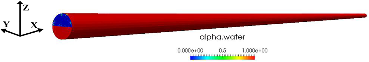
FIGURE 2. Geometric model of 3D horizontal pipe.

The height ratio of the inlet layer is 0.5. Air and water enter the horizontal pipeline through the blue and red inlet cross-sections (as indicated in Figure 1), respectively, at constant flow rates. The outlet is at standard atmospheric pressure. The model used the Newtonian fluid viscosity and Brackbill (Brackbill et al., 1992) continuous interface force (CFS) models. The phase interfacial tension per unit length was defined as 0.07 N/m with reference to Wang Xin’s fluid slug tracking model (Wang, 2006). The model uses OpenFOAM’s unique PIMPLE algorithm (Robertson et al., 2015), that is, the SIMPLE algorithm was used to solve the Navier-Stokes equations, and each time step was regarded as steady-state flow and was solved using the pressure implicit split operator (PISO) algorithm.

Turbulence Model

Choosing a reasonable turbulence model is the key to obtaining numerical simulation results which are consistent with the experimental results. Of the available turbulence models, the Direct Numerical Simulation model and Large Eddy Simulation model have low calculation efficiencies. The turbulence models commonly used in two-phase flow simulations include standard k-ε models, RNG k-ε models, realizable k-ε models, and k-εSST models. Here, V_sg = 3 m/s and V_sl = 1 m/s were used as input parameter values to evaluate the four turbulence models under the same grid number and time step. The models were used to simulate slug flow in the horizontal pipe section, and the results for slug formation distance and liquid slug frequency along the flow direction were compared with experimental data, as shown in Figures 3, whence it can be seen that the calculation examples from the realizable k-ε model were the closest to the experimental results and have a good degree of consistency. Therefore, the realizable k-ε model was selected as the turbulence model.

FIGURE 3

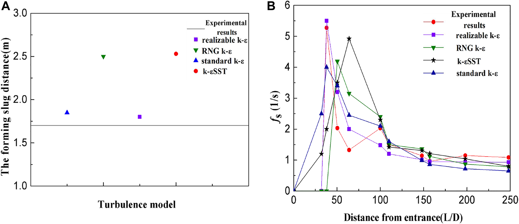
FIGURE 3. Comparison between simulated and experimental values of (A) slug formation position and (B) slug frequency by different turbulence models.

Grid, Time Step Independence Analysis

In order to capture the transient characteristics of the gas-liquid interface in the calculations, the Courant number was set at < 0.5. The value of the spatial step size Δx was fixed, and the time step size Δt was automatically adjusted according to the maximum phase velocity, U_max, obtained in each calculation time layer.

$Co=\frac{\left|U_{\max }\right|\Delta t}{\Delta x}\le 0.5(4)$

As in the previous section, V_sg = 3 m/s and V_sl = 1 m/s were taken as input values, and Courant numbers were simulated at the same spatial steps of 0.125, 0.25, 0.375, and 0.5, as shown in Figure 4, whence it can be seen that the time step has little effect on the simulation results. Hence, in order to improve the calculation efficiency, the time step at a Courant number of 0.5 was selected.

FIGURE 4

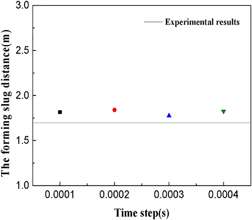
FIGURE 4. Variation of slug formation position with time step.

Here, a boundary layer encrypted hexahedral mesh was used to divide the geometric model, as shown in Figure 5. In order to eliminate the influence of grid sparsity on the results, simulations were conducted using spatial steps of 0.0025 m, 0.003 m, 0.0035 m, and 0.004 m (with the same V_sg and V_sl values as previously). The results are shown in Figure 6, whence it can be seen that the smaller the grid size, the closer the slug formation distance is to the experimental value. Simultaneously, the consistency of the simulated liquid slug frequency with the experimental value at different positions along the flow direction improves initially, before deteriorating as the number of grids becomes smaller. But when the spatial step is too small, the simulation accuracy is not accurate. This may be due to the fact that when the grid size is small, the frequent transmission of information between the grids leads to increased errors, which makes the simulations inconsistent with real slug flow. Therefore, a smaller spatial step size is not clearly better, and hence a spatial step size of 0.003 m was ultimately chosen.

FIGURE 5

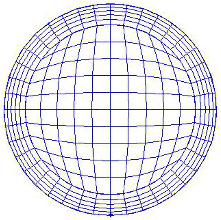
FIGURE 5. Grid structure for geometric model.

FIGURE 6

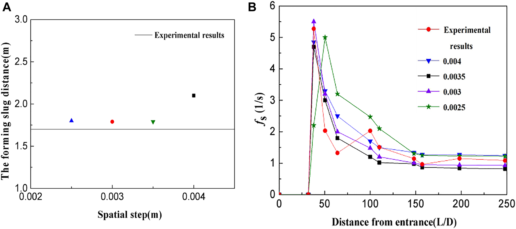
FIGURE 6. Comparison between simulated and experimental values of (A) slug formation position and (B) slug frequency by different spatial steps.

Model Validation

The numerical model was validated by simulating the two-phase flow of gas and water under different velocity conditions for a pipe with an inner diameter of 50 mm. Figure 7 shows a comparison between the five different flow patterns generated by the simulation and the corresponding experimental data, whence it can be seen that the simulated flow pattern is consistent with the experiments and appears to qualitatively reflect the characteristics of the phase interface structure of the two-phase flow at different gas-liquid speeds.

FIGURE 7

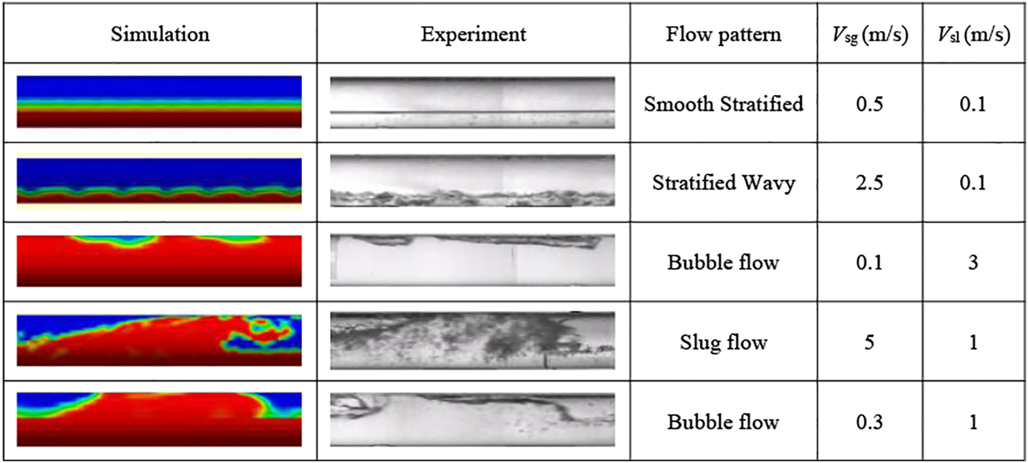
FIGURE 7. Comparison of simulation and experiments for five kinds of flow patterns.

The validated 3D model was then used to simulate the two-phase flow in the pipe geometry shown in Figure 2 at different gas and liquid velocities. The apparent velocity range of the gas phase was 0.1–6.5 m/s, and that of the liquid phase was 0.05–2 m/s, with a total of 148 data points chosen. A logarithmic coordinate system was used, whereby the abscissa and the ordinate represent the apparent velocities of the gas and liquid phases, respectively. The simulated operating conditions were drawn superimposed on a Mandhane flow pattern diagram according to the type of flow pattern, as shown in Figure 8. The red, blue, purple, and green points represent the operating points where the flow pattern simulation results are Bubble flow, Slug flow, Smooth Stratified flow and Stratified Wavy flow. The simulated operating points of Bubbly flow, Slug flow, and Smooth Stratified flow are consistent with the Mandhane flow pattern diagram. Taking slug flow as an example, the simulation result shows that among 57 operating points of the slug flow, 56 operating points are located in the slug flow area of the Mandhane flow pattern, and the accuracy rate is 98.2%. The Stratified Wavy flow has poor consistency with the Mandhane flow pattern diagram. This is because the Stratified Wavy flow area is small and the simulated operating points are few. In general, the simulation results are consistent with the Mandhane flow pattern diagram, which indicates the reliability of the model for two-phase flow simulations.

FIGURE 8

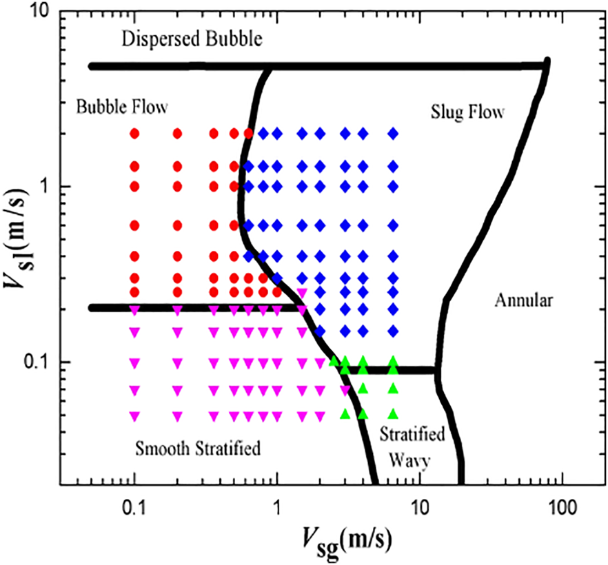
FIGURE 8. Comparison between flow pattern simulations and Mandhane flow pattern diagram.

Figure 9 shows the comparison between simulation value and experimental value of slug frequency under different working conditions (L/D = 258). It can be seen that the simulation value under high gas velocity are consistent with the experiment, and the simulation value under low gas velocity have a certain gap with the experimental value. When the gas velocity is constant, the slug frequency increases as the liquid velocity increases.

FIGURE 9

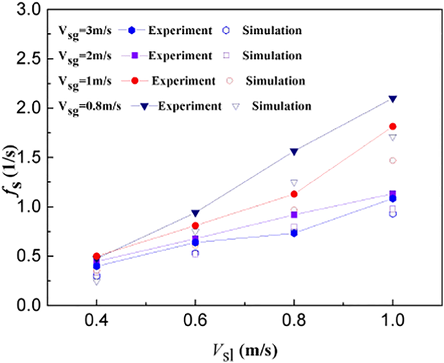
FIGURE 9. Comparison between simulation value and experimental value of slug frequency (L/D = 258).

Figure 10 shows a comparison between the simulated and experimental liquid slug frequency changes along the flow direction for V_sg = 3 m/s and V_sl = 1 m/s. From the figure, it can be seen that the simulated slug frequency closer to the inlet slightly overpredicts the experimental result. This is because the model assumes that the gas is incompressible, and that the change in inlet pressure, which is an important contributor to slug formation but has little effect on fully developed liquid slugs, will be directly transmitted to the downstream pipeline. The model results are quantitatively consistent with the experiments, and seem to reflect the natural development process of liquid slug formation, merger, and disappearance, thereby demonstrating the effectiveness of the model for slug flow simulation.

FIGURE 10

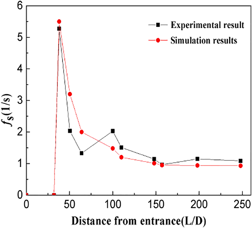
FIGURE 10. Comparison between simulations and experiments of slug frequency along the flow direction (V_sg = 3 m/s, V_sl = 1 m/s).

Simulation Results and Discussion

Characteristics of Slug Formation

Figure 11 shows a comparison of 2D simulation and experimental data of the slug formation process at the pipe entrance for V_sg = 2 m/s and V_sl = 0.2 m/s. It can be seen from the figure that a series of interface waves with high frequency and small amplitude are formed under the flowing gas. The momentum transfer between the gas and liquid causes the interface to become unstable, and the interface waves merge with each other, reducing the interface wave frequency and increasing the amplitude. When the cross-sectional area of the upper gas flow becomes smaller, the gas accelerates through the highest point of the interface wave. Due to the Bernoulli effect, the pressure of the gas above the interface wave decreases. When the pressure difference between the phases overcomes the interfacial tension and gravity, the interface wave is elevated. The slug formation phenomenon occurs when the crest of the interface wave blocks the pipeline. In both the experimental data and the simulations, the top of the interface wave is thrown forward by the gas velocity, forming the head of the thrown liquid slug.

FIGURE 11

FIGURE 11. Comparison between simulations and experiments of the slug formation process at the pipe entrance (Vsg = 2 m/s, Vsl = 0.2 m/s).

Characteristics of Liquid Slug Motion

Figure 12 shows a distribution diagram of the retention rate of a developing liquid slug for V_sg = 2 m/s and V_sl = 1 m/s, with a time interval of 0.05 s between each graph. For graphs (1)–(7) It can be seen that during the development of the liquid slug, the head of the slug is thrown forward and falls under the action of gravity. As a result, it sucks up the upstream liquid film, causing the slug length to increase. Simultaneously, the head of the liquid slug draws liquid into the bubbles with larger volume, causing these bubbles to gradually become smaller with the liquid slug motion and move to the tail of the slug, where they are finally discharged, before the next cycle of circulation, as shown in graphs (8)–(16). As the figure shows, it is due to this development process that the liquid slug head contains a much greater gas content than that in the tail.

FIGURE 12

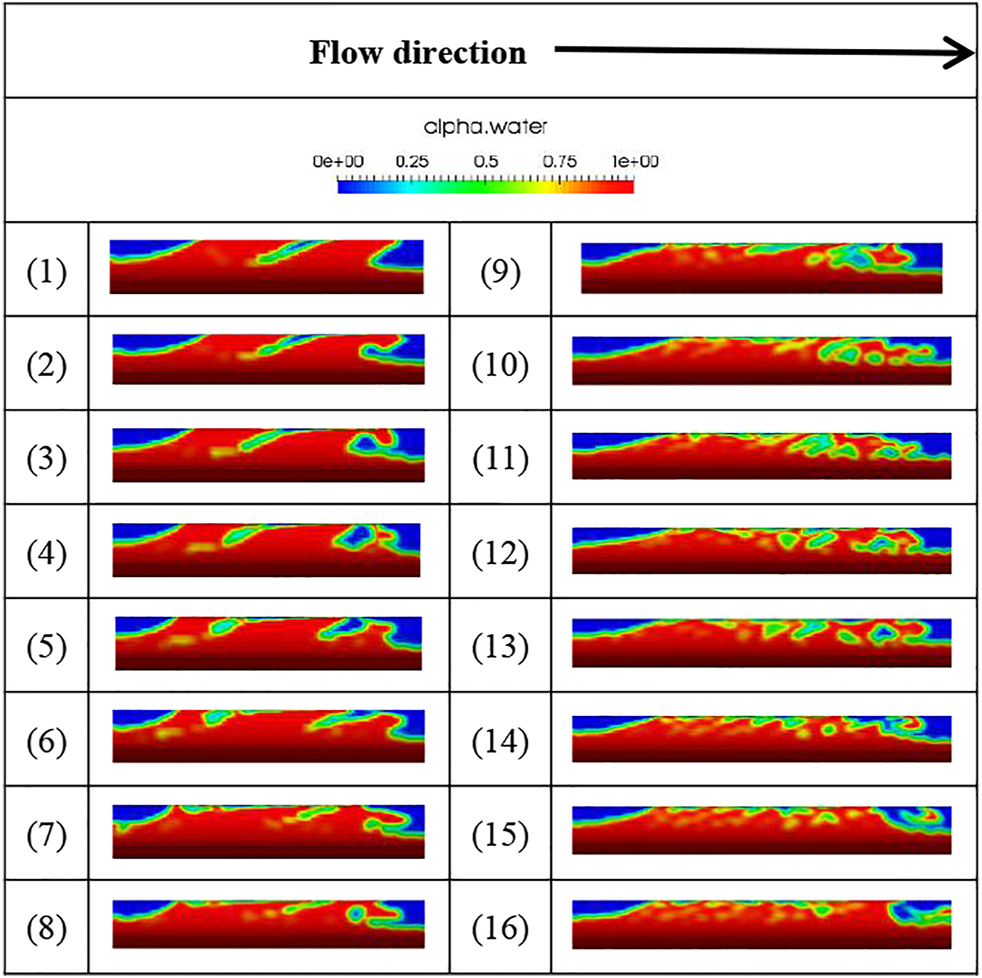
FIGURE 12. Liquid holdup distribution of a developing slug (V_sg = 2 m/s, V_sl = 1 m/s).

Figure 13 shows the displacement of a liquid slug changing with time for a constant V_sl of 1 m/s and V_sg values of 1, 2, and 3 m/s. It can be seen from the figure that increasing V_sg causes the liquid slug holding rate and the length of the liquid slug to decrease significantly, while the degree of ‘head throwing’ of the liquid slug increases. When the gas-liquid speed difference is small, the liquid level is high; hence, the liquid slug body is long and the throwing phenomenon of the liquid slug head is not obvious. Here, the liquid slug is moved forward by the gas in a balanced manner, absorbing the liquid film in front. When the gas-liquid speed difference is large, however, the throwing phenomenon is clearly evident, with the liquid slug advancing the liquid film through the periodic throwing and falling motion. This is because when the gas and liquid velocity difference is large, the liquid level is low and the amount of liquid slug is small. At high air flow speeds, the head of the liquid slug is thrown forward, causing a gap to form between the liquid and the upper part of the tube, and the gas accelerates through. The resulting pressure difference causes the liquid to be lifted and thrown forward, and the developing liquid slug circulates and moves forward in this way.

FIGURE 13

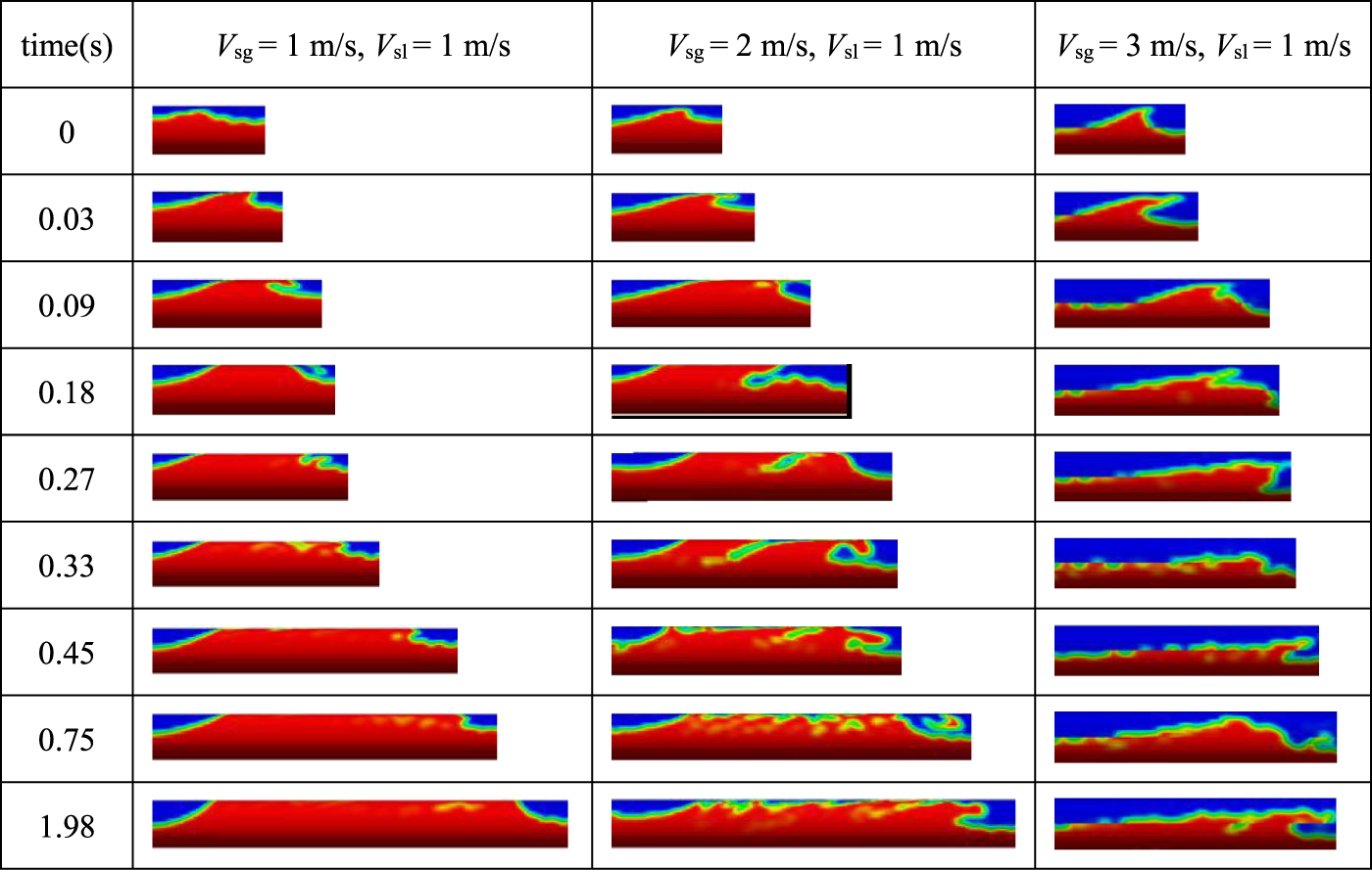
FIGURE 13. Variation of a developing slug with time with increasing gas-liquid speed difference.

Figure 14 shows the displacement of a fully developed liquid slug changing with time for a constant V_sl of 1 m/s, and V_sg values of 1 and 3 m/s. The figure shows that as V_sg increases, the liquid slug gas content increases significantly and degree of throwing of the liquid slug head increases. Compared to Table 2, it is evident that the characteristics of the fully-developed liquid slug motion are very different from that of the developing liquid slug, with fully-developed liquid slug head not displaying any periodic throwing and falling. Further, it appears that the difference in gas-liquid speed has no obvious effect on the fully-developed liquid slug’s movement and that the volume of liquid entrained by the liquid slug head is equal to the discharge volume of the tail. Hence, the length is kept stable, and the liquid slug moves forward evenly with its head thrown forward.

FIGURE 14

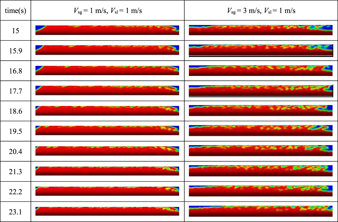
FIGURE 14. Variation of a fully-developed slug with time with increasing gas-liquid speed difference.

Transient Characteristics of the Liquid Slug Interface

In the simulations, the phenomenon of the head of the liquid slug being thrown forward and sucking in gas was observed, which is consistent with the structure of the actual liquid slug head from the high-definition photographs. Figure 15C shows that after the liquid slug is formed, the pressure behind it rises sharply, as evidenced by the effect of the pressure difference between the front and back of the slug. As a result, the liquid at the top of the slug is pushed out quickly, causing the head of the slug to be thrown forward, as the kinetic energy of the slug body is greater than that of the front liquid film area, as shown by the color of the vector arrows in Figure 15A. When the slug absorbs liquid from the film, this liquid is accelerated to the speed of the slug, thus forming a vortex zone at the slug’s front end. Due to the existence of the vortex, the liquid slug will entrain part of the gas, eventually forming a gas-liquid mixing zone with high kinetic energy at the head of the slug. This is consistent with the physical model of the shortest liquid slug length proposed by Dukler et al. (1985) in that the liquid slug speed is greater than the liquid film speed. Assuming that the slug is stationary, it is equivalent to the front liquid film jet entering the slug and forming a vortex in the area between the liquid film separation point and the return point, accompanied by a large number of air bubbles. This area is the liquid slug mixing area.

FIGURE 15

FIGURE 15. (A) Comparison between experimentally obtained slug head image and simulated velocity vectors. (B) Distribution of liquid holdup in the pipe cross-section. (C) Pressure distribution in the pipe before and after the slug.

Figure 16 shows the velocity distribution curves at different positions along a liquid slug during and after full development for V_sg = 1 m/s and V_sl = 1 m/s. For the developing liquid slug, the velocity of the upper part of the liquid gradually increases from the tail to the head of the slug, while the velocity of the lower part of the liquid gradually decreases. Figure 16A shows that the velocity distribution of the liquid slug during development is uneven, with the velocity in the upper half being greater than that in the lower half, particularly at x = 7.22 m, which is the liquid slug head. For fully developed liquid slugs, the velocity distribution is more uniform. The difference in the local maximum velocity between the slug tail and slug head area is 25.1%. Comparing Figures 16A,B, both the developing and fully-developed liquid slug heads are thrown forward, which is consistent with the analyses from Figures 13, 14.

FIGURE 16

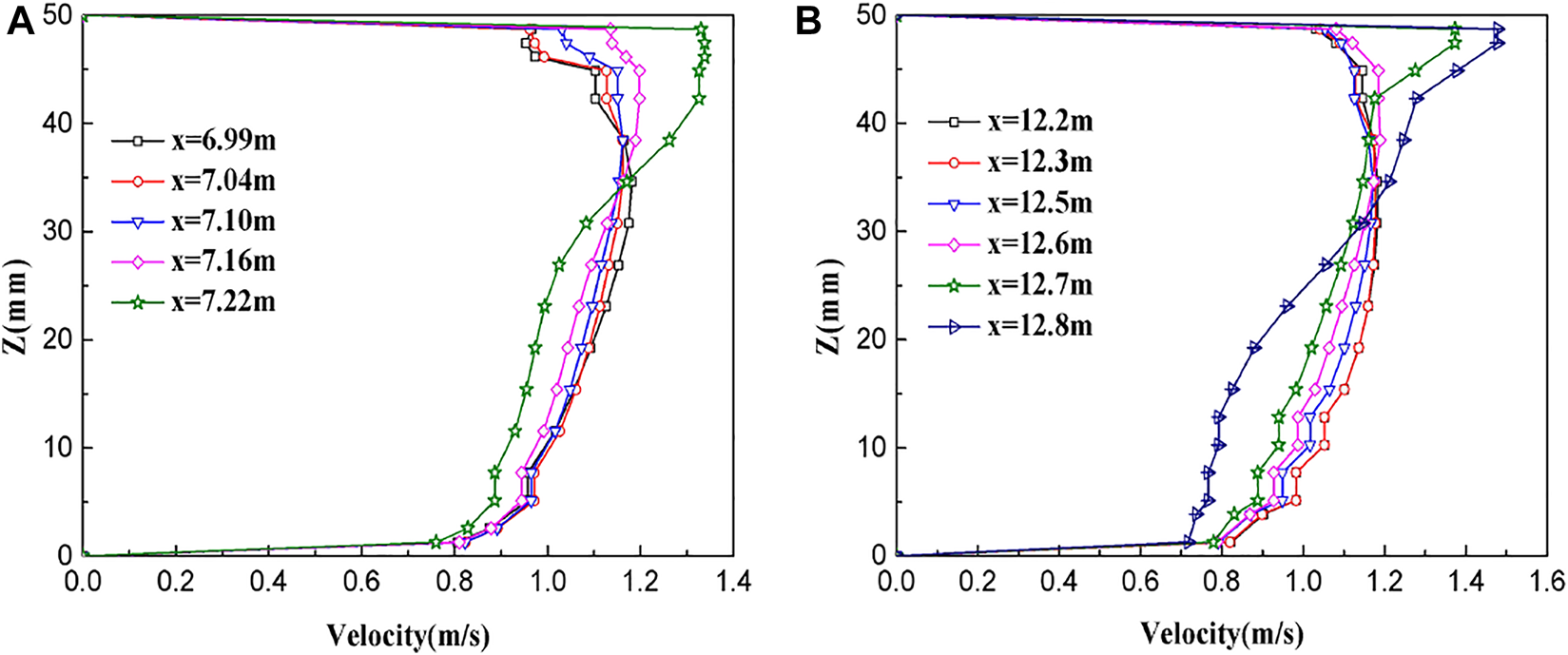
FIGURE 16. Velocity distribution curves of (A) developing and (B) developed slugs (V_sg = 1 m/s, V_sl = 1 m/s).

It can be seen from the velocity distribution curves that the velocity values near the bottom wall of the pipeline are similar. As the liquid slugs move downstream, the slug tail and body area have very similar velocity profiles, especially in the lower half region of the pipe regardless of the location.

Figure 17 shows the velocity distribution curves at different positions along a liquid slug during and after full development for V_sg = 2 m/s and V_sl = 1 m/s, which are consistent with those in Figure 16; however, compared to Figure 16, the increase in gas velocity makes the difference between the upper and lower speeds of the developing and the fully-developed slug increase significantly. The speed change of the slug head is particularly significant, and the difference in the local maximum velocity between the slug tail and slug head area is 33.5%. The result shows that the gas velocity has a significant effect on the liquid slug velocity distribution, i.e., the greater the gas velocity, the greater the velocity difference between the upper and lower of the liquid slug and the head and tail of the liquid slug.

FIGURE 17

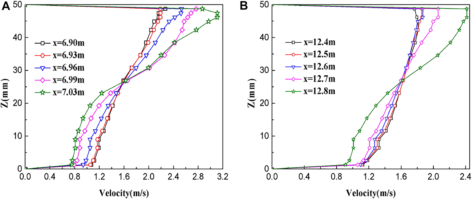
FIGURE 17. Velocity distribution curve of (A) developing and (B) developed slugs (V_sg = 2 m/s, V_sl = 1 m/s).

Figure 18 shows a cloud diagram of the cross-sectional velocity distribution of a developing and a fully-developed liquid slug for V_sg = 2 m/s and V_sl = 1 m/s. The position of the cross section is determined by dividing the liquid slug into equal parts along the flow direction. As the table shows, the velocity distribution of the fully-developed slug is more uniform, which is consistent with Figure 17. For the developing liquid slug, however, the velocity distribution is much more uneven, with the liquid velocity in the upper part of the slug being greater than that in the lower part. The velocity of the liquid from the tail to the upper part of the head of the slug gradually increases until it approaches the mixing speed of the gas and liquid phases. The velocity of the lower liquid gradually decreases to slightly lower than the velocity of the liquid film, which is the result of the combined action of pushing by the gas and the shear forces between the gas-liquid phase and the wall surface. Therefore, the speed of the liquid slug during development is mainly determined by the liquid velocity in its upper half. The formation and development of the liquid slug can be described as follows: the disturbance caused by the difference in the gas-liquid velocity at the pipeline inlet forms an interface wave, which merges and grows. Due to the limitations of the enclosed space in the pipeline, the bridge slug eventually forms a liquid slug, which moves forward in a way similar to interface wave.

FIGURE 18

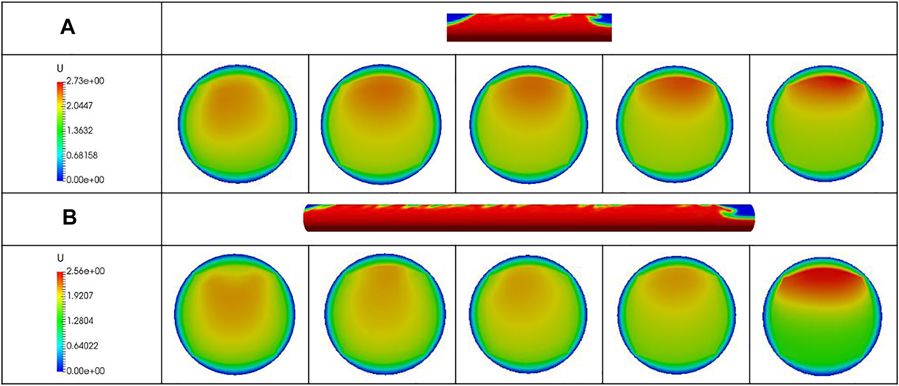
FIGURE 18. Cross-sectional flow distributions in (A) a developing and (B) a fully-developed slug (V_sg = 2 m/s, V_sl = 1 m/s).

Figure 19 shows the relative pressure distribution curves of the central axis of the pipeline from the inlet to the outlet at a certain moment under different working conditions, with corresponding pressure distribution cloud diagrams shown in Figure 20. These data show that the pressure decreased from the inlet to the outlet of the pipeline, and the convex shape in Figure 19 represents the liquid slug. As the gas pushes the liquid slug, the pressure from the liquid film area to the liquid slug tail shows a sudden increase. The energy loss of the viscous fluid in the flow process causes the pressure from the liquid slug tail to head gradually decrease. From the liquid slug head to the downstream liquid film area, a sudden drop in pressure occurs, due to the head of the liquid slug accelerating the front liquid film. Subsequently, the pressure in the liquid film does not change much. Therefore, it may be inferred that the pressure surge at the tail of the liquid slug is the main reason for the pressure fluctuations and vibrations in the pipeline. Through the quantitative analysis of Figure 20, it is found that as the liquid velocity increases, the pressure rise value from the upstream liquid film area to the liquid slug tail will increase, and the pressure drop value from the liquid slug head to the downstream liquid film area will increase accordingly, the pressure drop value caused by the liquid slug is about twice the pressure rise value at the tail of the slug, and it is mainly caused by the pressure drop at the head of the liquid slug, which is much higher than the normal hydraulic gradient. Therefore, the generation of slugs will increase the pressure energy loss of the entire pipeline.

FIGURE 19

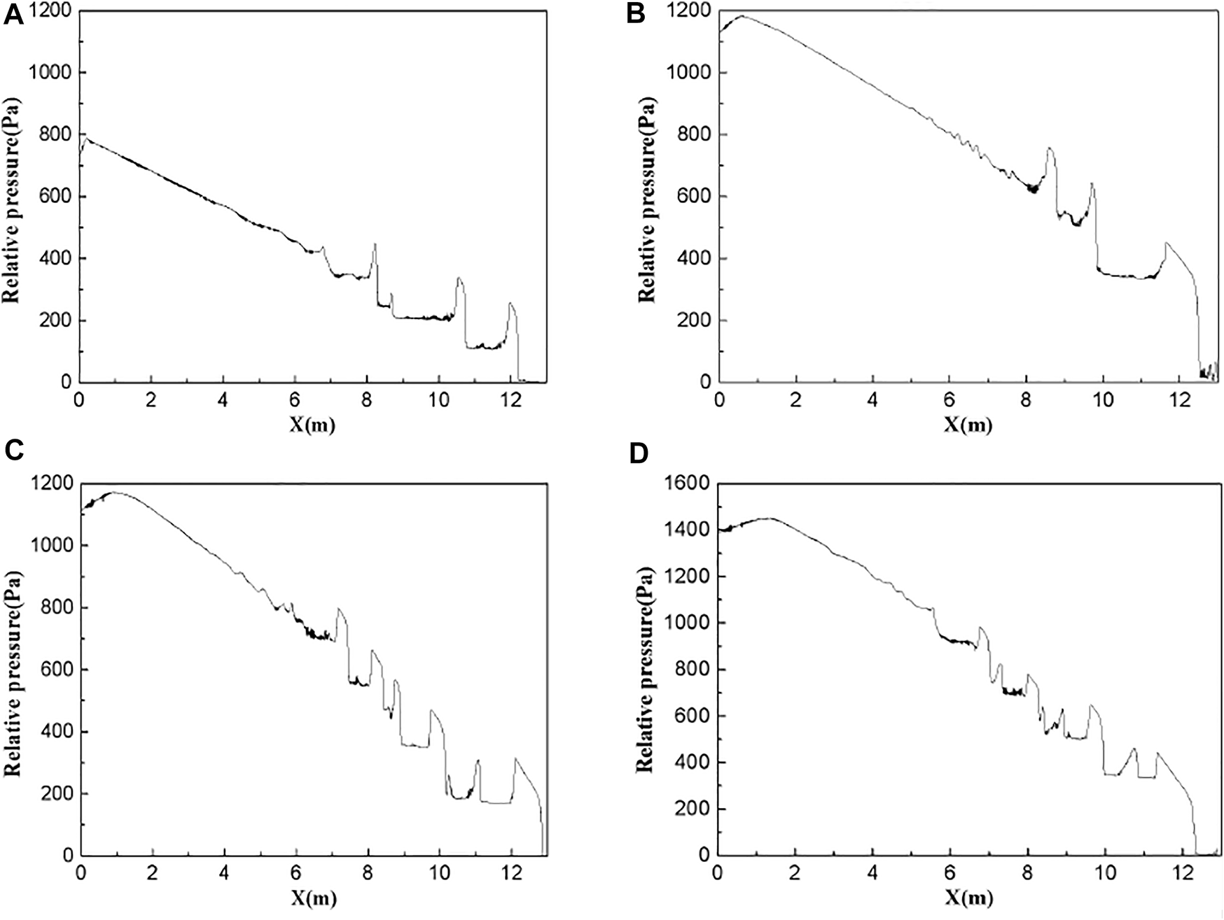
FIGURE 19. Relative pressure distribution curves of the central axis of the pipeline at a certain moment under the following flow conditions: (A) V_sg = 1 m/s, V_sl = 0.6 m/s, (B) V_sg = 1 m/s, V_sl = 0.8 m/s, and (C) V_sg = 1 m/s, V_sl = 1 m/s. (D) V_sg = 1 m/s, V_sl = 1.2 m/s.

FIGURE 20

FIGURE 20. Pressure distribution of a fully-developed slug at different liquid velocities.

Conclusion

1) Driven by the gas, a series of interface waves with high frequency and small amplitude are formed at the entrance of the pipeline. The instability of the interface causes the interface waves to merge with each other, reducing the interface wave frequency and increasing the wavelength and amplitude. When the crest of the interface wave blocks the pipeline, a slugging phenomenon occurs. Under the impulse of gas, the speed of the liquid slug head is greater than the speed of the front liquid film. The liquid slug head is thrown forward, forming a vortex at the junction of the liquid slug head and the front liquid film, and entraining a large amount of gas to form a liquid slug mixing area.

2) In the development of the liquid slug, when the gas-liquid speed difference is small, the liquid slug does not have a pronounced head, and it moves forward in a balanced manner under the force of the gas. When the gas-liquid speed difference is large, the head of the liquid slug is clearly thrown out, and it is pushed forward by the periodic throwing and falling motion. However, the fully-developed liquid slug head does not exhibit this periodic throwing and falling. Additionally, the difference in gas-liquid speed has no obvious effect on the form of the liquid slug, which moves forward evenly by throwing its head forward. With the increase in the superficial velocity of the gas phase, the gas content of the developing and fully-developed liquid slugs increase significantly, which causes the degree of head ejection of the liquid slug as well as the difference between its upper and lower speeds to increase.

3) The velocity distribution of the liquid slug during development is uneven, and the slug continuously moves forward through entraining liquid in the head and discharging it in the tail. The overall velocity field distribution becomes more uniform after fully-developed. The slug tail and body area have very similar velocity profiles, especially in the lower half region of the pipe regardless of the location.

4) The pressure from the upstream liquid membrane area to the end of the slug suddenly increases, while that from the end of the slug to its head gradually decreases, and the pressure from the slug head to the downstream liquid membrane area suddenly drops. The pressure drop value caused by the liquid slug is about twice the pressure rise value at the tail of the slug, and it is mainly caused by the pressure drop at the head of the liquid slug, which is much higher than the normal hydraulic gradient. The sudden pressure rise in the slug tail is the main cause of pipeline pressure fluctuations and pipeline vibration.

Data Availability Statement

The original contributions presented in the study are included in the article/Supplementary Material, further inquiries can be directed to the corresponding author.

Author Contributions

XW put forward research ideas and formulated or formed overall research objectives; ZWprovided experimental data and led research activities; MD integrated literature and data; LD reviewed and modified the article; QG received financial support for the publication project.

Funding

This work was supported by Science Development Funding Program of Dongying, Grant No. DJ2020009. Qingdao Nuocheng Chemical Safety Technology Co., Ltd. is jointly funded by the chemical registration center of emergency management department and China Chemical Safety Association. The company mainly provides enterprises with “one-stop solutions” in the fields of safety consulting, environmental protection management, emergency and fire protection technology, chemical management and so on, and creates a comprehensive HSSE product and technical service model.

Conflict of Interest

MD was employed by Qingdao Nuocheng Chemical Safety Technology Co., Ltd.

The remaining authors declare that the research was conducted in the absence of any commercial or financial relationships that could be construed as a potential conflict of interest.

Publisher’s Note

All claims expressed in this article are solely those of the authors and do not necessarily represent those of their affiliated organizations, or those of the publisher, the editors and the reviewers. Any product that may be evaluated in this article, or claim that may be made by its manufacturer, is not guaranteed or endorsed by the publisher.

References

Abdulkadir, M., Hernandez-Perez, V., Lo, S., Lowndes, I. S., and Azzopardi, B. J. (2013). Comparison of Experimental and Computational Fluid Dynamics (CFD) Studies of Slug Flow in a Vertical 90° Bend. The J. Comput. Multiphase Flows 5 (4), 265–281. doi:10.1260/1757-482x.5.4.265

CrossRef Full Text | Google Scholar

Bonizzi, M. (2003). Transient One-Dimensional Modeling of Multiphase Slug Flows. London: Imperial College London. Doc.S.Dissertation.

Google Scholar

Brackbill, J. U., Kothe, D. B., and Zemach, C. (1992). A Continuum Method for Modeling Surface Tension. J. Comput. Phys. 100 (2), 335–354. doi:10.1016/0021-9991(92)90240-Y

CrossRef Full Text | Google Scholar

De Schepper, S. C. K., Heynderickx, G. J., and Marin, G. B. (2008). CFD Modeling of All Gas-Liquid and Vapor-Liquid Flow Regimes Predicted by the Baker Chart. Chem. Eng. J. 138 (1), 349–357. doi:10.1016/j.cej.2007.06.007

CrossRef Full Text | Google Scholar

Deendarlianto, Andrianto, M., Widyaparaga, A., Dinaryanto, O., Khasani, F., and Indarto, C. (2016). CFD Studies on the Gas-Liquid Plug Two-phase Flow in a Horizontal Pipe. J. Pet. Sci. Eng. 147, 779–787. doi:10.1016/j.petrol.2016.09.019

CrossRef Full Text | Google Scholar

Dukler, A. E., Moalem Maron, D., and Brauner, N. (1985). A Physical Model for Predicting the Minimum Stable Slug Length. Chem. Eng. Sci. 40 (8), 1379–1385. doi:10.1016/0009-2509(85)80077-4

CrossRef Full Text | Google Scholar

Ekambara, K., Sanders, R. S., Nandakumar, K., and Masliyah, J. H. (2008). CFD Simulation of Bubbly Two-phase Flow in Horizontal Pipes. Chem. Eng. J. 144 (2), 277–288. doi:10.1016/j.cej.2008.06.008

CrossRef Full Text | Google Scholar

Glatzel, T., Litterst, C., Cupelli, C., Lindemann, T., Moosmann, C., Niekrawietz, R., et al. (2008). Computational Fluid Dynamics (CFD) Software Tools for Microfluidic Applications - A Case Study. Comput. Fluids 37 (3), 218–235. doi:10.1016/j.compfluid.2007.07.014

CrossRef Full Text | Google Scholar

Ishii, M. (2006). Thermo-fluid Dynamic Theory of Two-phase Flows. Springer New York Press.

Google Scholar

Lu, M. (2015). Experimental and Computational Study of Two-phase Slug Flow. UK: Imperial College London. Doc.S.Dissertation.

Google Scholar

OpenFOAM (2019). OpenFOAM User Guide, V6. London, United Kingdom: Henry Weller.

Google Scholar

Ramdin, M., and Henkes, R. A. W. M. (2011). “CFD for Multiphase Flow Transport in Pipelines,” in ASME. International Conference on Ocean, Offshore and Arctic Engineering, 377–387. doi:10.1115/omae2011-49514

CrossRef Full Text | Google Scholar

Ramdin, M., and Henkes, R. (2012). Computational Fluid Dynamics Modeling of Benjamin and Taylor Bubbles in Two-phase Flow in Pipes. J. Fluid Eng-t. ASME. 134 (4), 041303. doi:10.1115/1.4006405

CrossRef Full Text | Google Scholar

Ratkovich, N., Chan, C. C. V., Berube, P. R., and Nopens, I. (2009). Experimental Study and CFD Modelling of a Two-phase Slug Flow for an Airlift Tubular Membrane. Chem. Eng. Sci. 64 (16), 3576–3584. doi:10.1016/j.ces.2009.04.048

CrossRef Full Text | Google Scholar

Robertson, E., Choudhury, V., Bhushan, S., and Walters, D. K. (2015). Validation of OpenFOAM Numerical Methods and Turbulence Models for Incompressible bluff Body Flows. Comput. Fluids 123, 122–145. doi:10.1016/j.compfluid.2015.09.010

CrossRef Full Text | Google Scholar

Taitel, Y., Sarica, C., and Brill, J. P. (2000). Slug Flow Modeling for Downward Inclined Pipe Flow: Theoretical Considerations. Int. J. Multiphase Flow 26 (5), 833–844. doi:10.1016/S0301-9322(99)00053-1

CrossRef Full Text | Google Scholar

Vallée, C., Höhne, T., Prasser, H.-M., and Sühnel, T. (2008). Experimental Investigation and CFD Simulation of Horizontal Stratified Two-phase Flow Phenomena. Nucl. Eng. Des. 238 (3), 637–646. doi:10.1016/j.nucengdes.2007.02.051

CrossRef Full Text | Google Scholar

Vallée, C., Lucas, D., Beyer, M., Pietruske, H., Schütz, P., and Carl, H. (2010). Experimental CFD Grade Data for Stratified Two-phase Flows. Nucl. Eng. Des. 240 (9), 2347–2356. doi:10.1016/j.nucengdes.2009.11.011

CrossRef Full Text | Google Scholar

Wang, X. (2006). Investigation of Two-Phase and Multiphase Slug Flow in Horizontal Pipe and Multiphase Slug Flow and Ascending Pipe System. China: Xi’an Jiaotong University. Doc.S.Dissertation.

Google Scholar

Yin, P., Zhang, P., Cao, X., Li, X., Li, Y., and Bian, J. (2022). Effect of SDBS Surfactant on Gas-Liquid Flow Pattern and Pressure Drop in Upward-Inclined Pipelines. Exp. Therm. Fluid Sci. 130, 110507. doi:10.1016/j.expthermflusci.2021.110507

CrossRef Full Text | Google Scholar

Zheng, G., Brill, J. P., and Taitel, Y. (1994). Slug Flow Behavior in a Hilly Terrain Pipeline. Int. J. Multiphase Flow 20 (1), 63–79. doi:10.1016/0301-9322(94)90006-X

CrossRef Full Text | Google Scholar