A Machine Learning-Based Model Predictive Control Method for Pumped Storage Systems

Integrated systems required for renewable energy use are under development. These systems impose more stringent control requirements. It is quite challenging to control a pumped storage system (PSS), which is a key component of such power systems. Because of the S-characteristic area of the PSS pump turbine, traditional proportional-integral-derivative (PID) control induces considerable speed oscillation under medium and low water heads. PSSs are difficult to model because of their nonlinear characteristics. Therefore, we propose a machine learning (ML)-based model predictive control (MPC) method. The ML algorithm is based on Koopman theory and experimental data that includes PSS state variables, and is used to establish linear relationships between the variables in high-dimensional space. Subsequently, a simple, accurate mathematical PSS model is obtained. This mathematical model is used via the MPC method to obtain the predicted control quantity value quickly and accurately. The feasibility and effectiveness of this method are simulated and tested under various operating conditions. The results demonstrate that the proposed MPC method is feasible. The MPC method can reduce the speed oscillation amplitude and improve the system response speed more effectively than PID control.

Introduction

Sustainable energy has become increasingly important due to the present-day shortage of and pollution from fossil fuels (Albuyeh, 2013; Menon, 2013; Bozchalui, 2015; Brahman and Jadid, 2015; Zhang et al., 2015; Güney, 2019; Hasan Mehrjerdi, 2021; Rajvikram Madurai Elavarasan et al., 2021; Thomas Sattich et al., 2021). Consequently, renewable power generation technologies such as wind, solar, hydro, and biomass are used widely (Rajkumar, 2011; Francesco Calise and Piacentino, 2014; Pazouki, 2014; Zhaoyang Dong and Wen, 2014; Pazouki, 2016; Elena Smirnova et al., 2021; Eric O Shaughnessy et al., 2021; Olusola Bamisile et al., 2021; Pradhan et al., 2021). Simultaneously, energy storage technologies such as fuel cells, hydrogen storage, supercapacitors, and pumped storage systems (PSSs) have attracted increasing attention (Yves Pannatier et al., 2010; Pazouki, 2014; Brahman and Jadid, 2015; Zhang et al., 2015; Pazouki, 2016; Li et al., 2017a; Schmidt et al., 2017). PSSs are an early form of modern energy storage and are important to the development of sustainable power systems. A PSS operates economically by generating electricity during peak demand periods and pumping water to storage tanks during off-peak periods; it thus plays an important role in the economical operation of conventional power systems and facilitates the efficient use of renewable energy (Gurung et al., 2016; van Meerwijk et al., 2016; Kocaman and Modi, 2017; Min and Kim, 2017; Ruppert et al., 2017; Sam and Gounden, 2017; Julian David Hunt et al., 2020).

As the scale of PSSs and the extent to which they are utilized in the development of sustainable power systems increase, their precise control has gradually emerged as an important area of research. Existing PSS control methods can be divided into two main categories. The methods within the first category use proportional-integral-derivative (PID) control. These methods are based mainly on parametric design of each link within the PID controller. Some representative studies follow.

Shi et al. used the d-q axis vector of a generator to design PI parameters with the aim of achieving highly efficient peak regulation and frequency suppression within a power grid (Yifeng Shi et al., 2020). Zhao et al. used the power priority control and speed priority control strategies to design PID parameters, in addition to simulating and verifying the superior control effect of the power control strategy (Yves Pannatier et al., 2010; Guopeng Zhao and Ren, 2021). Several other advanced algorithms and theories have been applied as well. Xu et al. designed a fuzzy PID controller based on the F fractional-order integrator and differentiator (FOPID) (Podlubny, 1999) by using a search algorithm. This controller optimizes the FOPID method parameters, increases the convergence speed, and yields superior results (Xu et al., 2016; Xu et al., 2018). Gao et al. used Hopf bifurcation theory to determine the algebraic stability criterion of a PSS in order to obtain ideal PID controller parameters that correspond to a stable system state (Chunyang Gao et al., 2021a).

The control methods under the second category use optimization algorithms to determine the best approach to coping with the nonlinear behaviors of hydraulic systems. Schmidt et al. used a nonlinear optimization algorithm to determine the best stationary operating point of a PSS in order to minimize loss across the entire system and consider operating constraints systematically (Schmidt et al., 2017). Hou et al. used a multiobjective optimization algorithm to design a control strategy for starting a PSS in addition to establishing a simulation model based on a real system to verify the feasibility of the optimized control strategy (Hou et al., 2018; Hou et al., 2019). Pan et al. modeled a new stability criterion by using the particle swarm algorithm to optimize the parameters of a PSS controller; this criterion enhanced the independent response of the PSS significantly (Pan et al., 2021).

Among the various optimization control methods, the model predictive control (MPC) method has a robust theoretical foundation and substantial promise for practical applications. The most famous explanation is called “Open Loop Optimal Feedback” (Alamir and Allgöwer, 2008; Diego and Carrasco, 2011; Forbes MG et al., 2015). It richly illustrates the four layers of modeling, control, optimization, and logistics in the MPC control method and their relationship (Mayne, 2016; Shiliang Zhang et al., 2017; Sopasakis and Sarimveis, 2017; Ye et al., 2017). In recent years, the application of MPC to PSSs has gradually attracted the attention of scholars. Li et al. used the generalized nonlinear predictive control method to design a PSS controller and simulated start-up and speed disturbance processes under no-load conditions to verify controller robustness and efficiency (Li et al., 2017b). Liang et al. proposed an MPC strategy based on enumeration to determine the optimal switching time of a PSS with the objectives of increasing operational flexibility and promoting frequency regulation (Liang et al., 2019). Feng et al. proposed a new adaptive MPC strategy and conducted a simulation experiment to verify the superiority of this strategy in terms of adjusting the voltage and load and suppressing frequency oscillation (Chen Feng et al., 2021). Although MPC has the above advantages, it still has certain disadvantages when compared to traditional control methods. For instance, MPC modeling requires more expert knowledge and is time-consuming to perform using traditional methods (De Souza et al., 2010; Max Schwenzer et al., 2021. Fortunately, the continuous development of hardware equipment and control algorithms has decreased the MPC control time. If the control effect is particularly important, MPC is much better than traditional control methods.

Modeling is a key component of MPC but almost all systems used in relevant contexts are nonlinear; for example, the water pump turbine of a PSS has an S-characteristic area (Yin et al., 2014; Li et al., 2017a; Anilkumar et al., 2017; Zeng et al., 2017; Zhang et al., 2017). This increases the difficulty of modeling. A variety of modeling methods have been developed in response.

Huang et al. proposed a method of predicting the complete characteristics of a Francis pump turbine. Based on Euler’s equation and the velocity triangle at the runner, their method derives a mathematical model that completely describes the characteristics of the Francis pump turbine. The results of a simulation experiment indicated that their method was suitable for performing a priori simulations before measuring device characteristics (Huang et al., 2018). Gao et al. established a high-precision, variable-speed control model for a pump turbine based on the complete characteristic curve of the turbine in order to describe the characteristics of the variable speed units more effectively (Chunyang Gao et al., 2021b). Zhou et al. proposed a real-time accurate equivalent circuit model of a PSS via error compensation. This model reconciles the conflict between real-time online simulation and simulation accuracy under various operating conditions (Jianzhong Zhou et al., 2018).

In recent years, with the continual development of artificial intelligence technology, a few machine learning (ML) algorithms have yielded outstanding nonlinear system modeling results (R. Martin et al., 2015; J. Sánchez Oro et al., 2016; Li et al., 2016; Idowu et al., 2016; Robinson et al., 2017; Yong Ping Zhao et al., 2018; Kiely et al., 2019; Ayush Thada et al., 2021). The application of ML algorithms to PSS has emerged as an innovative idea. In this regard, Feng et al. established a PSS model by optimizing the initial learning parameters via prior knowledge learning and subsequently adopting a stepped control strategy and an artificial-sheep-algorithm-based rolling optimization mechanism. This model can replace the existing differential geometry model (Chen Feng et al., 2021). Zhao et al. introduced an improved Suter transformation-backpropagation (BP) neural network interpolation model and used it to establish a PSS model. This model can be divided into three parts: characteristic curve processing, data prediction, and interpolation. It can correct the characteristic curve of a pump turbine effectively (Zhigao Zhao et al., 2019). These modeling methods are innovative and represent meaningful research directions. However, the model machines and BP neural networks used in the aforementioned modeling methods have extremely complex structures and use large numbers of parameters. This increases the complexity of PSS control.

For these reasons, we propose using a MPC method based on an ML algorithm to model PSS control. This method can convert a nonlinear model into a linear model in high-dimensional space. The form of the obtained model is simple and few parameters are required. Thus, it is suitable for fast, accurate control processes. Our paper makes the following contributions to PSS development: 1) The pump-turbine partition model that we establish effectively solves the common problem of difficult modeling in the S-region and provides a feasible direction for research on pump turbines in the s-region. 2) The machine-learning algorithm that we propose makes full use of the data generated in the PSS; it is an effective way of combining experimental data with the actual system and improves the accuracy of the actual system model. 3) We use the proposed model within the MPC method; this solves the problem of large control errors in the PSS at low water heads. 4) Compared to traditional control methods, our proposed method can reduce the shock of the pumped storage system and reduce the control process adjustment time.

PSS Modeling

The overall MPC structure is illustrated in Figure 1. It comprises three parts: a controlled system (a PSS), a data collection component, and a control component. The PSS is composed of a pump turbine, servo mechanism, penstock, and generator. The function of the data acquisition component is to collect the data in the PSS and provide it to the control system. It includes a flow sensor, a torque sensor, a speed sensor, an opening sensor, and a pressure gauge, and is responsible for collecting five variables: the flow, torque, speed, guide vane opening, and water head. The control system includes model generators for pumps, turbines, servo systems, pipelines, and generators. Their task is to generate PSS component models that the controller can use. The control system also includes a predictor that generates a predictive model. In addition, the controller generates control instructions according to the optimized algorithm in order to manipulate the PSS control variables.

FIGURE 1

FIGURE 1. The overall power storage system model predictive control structure.

Five important state variables are used in the PSS: $a$ is the vane opening, $n_{11}$ is the unit rotational speed, $Q_{11}$ is the unit flow, $M_{11}$ is the unit torque, and $h$ is the water head magnitude. The modeling process aims to establish the relationships between these state variables. The real values of these state variables at each moment are collected via digital equipment and used in the control process. The controller determines the optimal amount of control via the model prediction process and uses the optimizer to control the PSS.

ML Algorithm

To establish a simple, accurate PSS model, we propose an ML algorithm that can determine the linear relationships among state variables in high-dimensional space using the given data.

Related Principles

1) Assume that the set of all state variables $s^{\left(i\right)}$ is given in Eq. 1. To study the relationship between the state variables $s^{\left(u\right)}$ and $s^{\left(v\right)}$, we assume that they satisfy the relationship given in Eq. 2, the discrete form of which is given in Eq. 3. All of these relationships are nonlinear.

$S=\left\{s^{\left(i\right)}|i=\mathrm{1,2},\cdots ,N_s\right\},(1)$

where $s^{\left(i\right)}$ is the state variable in system; $N_s$ is the number of state variables.

$\frac{\partial s^{\left(u\right)}}{\partial s^{\left(v\right)}}=\mathrm{g}\left(s^{\left(u\right)}\right),(2)$

where $\partial s^{\left(u\right)},\partial s^{\left(v\right)}$ is the amount of change in $s^{\left(u\right)}$and $s^{\left(v\right)}$respectively; $\mathrm{g}\left(s^{\left(u\right)}\right)$ is a certain relational expression of $s^{\left(u\right)}$.

$s_{j+1}^{\left(u\right)}=\mathrm{G}\left(s_j^{\left(u\right)}\right),(3)$

where $s_j^{\left(u\right)},s_{j+1}^{\left(u\right)}$ is the value of $s^{\left(u\right)}$ at time $j$and $j+1$ respectively; $\mathrm{G}\left(s_j^{\left(u\right)}\right)$ is a certain discrete function of $s^{\left(u\right)}$ at time $j$.

For nonlinear relationships, Koopman proposed the Koopman operator (KO), expressed in Eq. 4, in 1931. The KO can be used to represent the complete nonlinear relationship using a linear function. Notably, no universal method is available for selecting the observation function; it is usually selected based on the characteristics of the system and the analyst’s experience.

$KO=O\circ \mathrm{G},(4)$

where $O\left(s\right)=\left[o_1\left(s\right),o_2\left(s\right),\dots ,o_p\left(s\right)\right]$ is the measure function acting on the state variables; $\circ$ represent a compound operation of functions.

2) For each value of $s^{\left(v\right)}$, there exists a corresponding dataset $s^{\left(u\right)}$, which can be expressed as a matrix, as in Eq. 5.

$DM=\left[\begin{array}{cccc}|& |& \cdots & |\\ s_1^{\left(u\right)}& s_2^{\left(u\right)}& \cdots & s_N^{\left(u\right)}\\ |& |& \cdots & \text{|}\\ s_1^{\left(v\right)}& s_2^{\left(v\right)}& \cdots & s_N^{\left(v\right)}\end{array}\right],(5)$

where $DM$ is data matrix composed of $N$ sets of values of state variables.

We apply the KO to matrix $DM$ to obtain the high-dimensional data matrix $K$, as shown in Eq. 6. Then, we take columns 1 through N-1 of $K$ as $K_a$ and columns 2 through N as $K_b$, as indicated in Eqs 7, 8, respectively.

$K=O\left(D\right)=\left[o_1\left(D\right),o_2\left(D\right),\dots ,o_p\left(D\right)\right]=\left[\begin{array}{cccc}|& |& \cdots & |\\ k_1& k_2& \cdots & k_N\\ |& |& \cdots & |\end{array}\right],(6)$

where $K$ is data matrix in measurement space that apply the measure function $\text{O}\left(s\right)$ to $DM$.

$K_a=\left[\begin{array}{cccc}|& |& \cdots & |\\ k_1& k_2& \cdots & k_{N-1}\\ |& |& \cdots & |\end{array}\right],(7)$

$K_b=\left[\begin{array}{cccc}|& |& \cdots & |\\ k_2& k_3& \cdots & k_N\\ |& |& \cdots & |\end{array}\right],(8)$

where $K_a,K_b$ is data matrix consisting of $N-1$ columns of $K$.

According to the Koopman principle, under a suitable observation function set, $K_b$ and $K_a$ share a linear relationship that can be expressed as Eq. 9. Therefore, the estimated value of $K_N$ can be calculated using Eq. 10.

$K_b=A\cdot K_a,(9)$

where $A$ is a steady matrix.

${\widehat{k}}_N=A\cdot k_0,(10)$

where ${\widehat{k}}_N$ is the estimated value of $k_N$; $k_0$is the initial value of matrix $K$.

The error is the deviation between the real value $k_N$ and the estimated value ${\widehat{k}}_N$, as shown in Eq. 11. If the selected measurement function can ensure that this error is smaller than a threshold that we set, $K_a$ and $K_b$ can be considered to have a linear relationship.

$error=\left|k_N-{\widehat{k}}_N\right|,(11)$

where $error$ is the error between the true value $k_N$ and the estimated value${\widehat{k}}_N$.

3) When $K_a$ and $K_b$ share a linear relationship under a certain observation function set, the relationship between $s^{\left(u\right)}$ and $s^{\left(v\right)}$can expressed using Eq. 12.

$s^{\left(u\right)}={\displaystyle \sum _{i=0}^p{f}_i\cdot o_i\left(s^{\left(v\right)}\right)},(12)$

where $f_i$ is an undetermined coefficient.

ML Algorithm Flow

The ML algorithm flow is depicted in Figure 2. It consists of the following parts: data preprocessing, KO, establishment of the objective equation, estimation of the state variable value, error calculation, parameter determination, and determination of the fit model. The details follow:

FIGURE 2

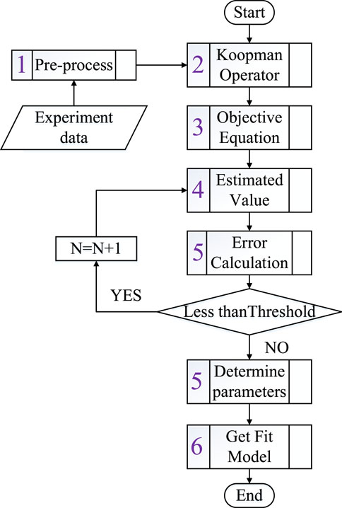
FIGURE 2. The ML algorithm flow.

Data Preprocessing

Experimental data are generated using the experimental platform. All $s^{\left(u\right)}$ versus $s^{\left(v\right)}$ experimental data are collected and sorted into a data matrix $D$, as expressed in Eq. 5.

KO

The observation function set is selected according to theoretical principles and practical experience and applied to matrix $D$ to obtain the high-dimensional spatial data matrix $K$. Then, we select the matrixes $K_a$ and $K_b$, each of which has N-1 columns, where N is a parameter that must be determined.

Establishing the Objective Equation

We establish the objective equation given in Eq. 9 and transform it into the form presented in Eq. 13.

$A=K_b\cdot K_a^{+},(13)$

where $K_a^{+}$ is the pseudo-inverse of $K_a$.

Calculation of the Estimated Value

We perform singular value decomposition on $K_a$ to obtain the decomposed form, as shown in Eq. 14.

$K_a=U\cdot \Sigma \cdot V^{\ast },(14)$

where $U\in {ℂ}^{n\times n}$ and $V\in {ℂ}^{m\times m}$ are unitary matrices, and $\Sigma \in {ℂ}^{n\times m}$ is a diagonal matrix.

Next, matrix A can be expressed using Eq. 15. Its eigenvalue decomposition form is given in Eq. 16.

$A=K_b\cdot V{\left(\Sigma \right)}^{-1}{\left(U\right)}^{\ast },(15)$

where ${\left(U\right)}^{\ast }$ is the conjugate matrix of $U$.

$AW=W\Lambda =W\left[\begin{array}{ccc}{\lambda }_1& & \\ & \ddots & \\ & & {\lambda }_k\end{array}\right],(16)$

where $W$ is the eigenvector matrix of A and $\Lambda$ is the eigenvalue matrix.

By substituting Eq. 15 into Eq. 16, we can obtain the linear model given in Eq. 17. The value of $K_N$ can estimated in this manner, as expressed in Eq. 18.

$\Phi =AW=K_b\cdot V{\left(\Sigma \right)}^{-1}{U}^{\ast }W=\left[\begin{array}{cccc}|& |& \cdots & |\\ {\varphi }_1& {\varphi }_2& \cdots & {\varphi }_{N-1}\\ |& |& \cdots & |\end{array}\right],(17)$

${\widehat{k}}_N=\Phi \cdot {\Lambda }^{k-1}\cdot k_0,(18)$

where $k_0={\Phi }^{+}\cdot k_1$ is the initial value of $k_N$.

Error Calculation and Parameter Determination

The error between the real and estimated values is expressed in the form given in Eq. 19. This expression is related to the parameter $N$. We gradually increase $N$ until the error exceeds the threshold. The minimum value of $N$ for which the error exceeds the threshold is set as the parameter value.

$error={\displaystyle \sum _{x=1}^N\left|k_x-\Phi \cdot {\Lambda }^{k-1}\cdot k_0\right|}.(19)$

Fit Model Determination

As previously mentioned, the form of the fitted model is given in Eq. 12. We use the least squares method to determine the coefficient $f_i$ in this equation.

PSS Models

Pump Turbine Modeling Using an ML Algorithm

The pump-turbine model contains s-shaped regions and is a complex, nonlinear model. We use machine learning algorithms to model the pump-turbine by partition. The process is shown in the Figure 3. A detailed description of the modeling process is provided below.

FIGURE 3

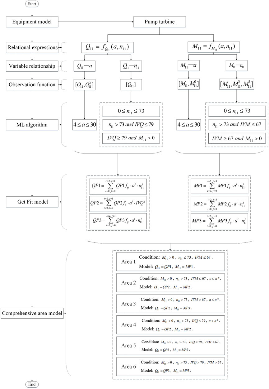
FIGURE 3. The partition modeling flowchart.

The pump turbine model is based on two relational expressions. That is, $a$and $n_{11}$ are used to express $Q_{11}$ and $M_{11}$ in the forms given in Eqs 20, 21, respectively. Notably, these are two nonlinear relationships and “S” regions are present. That is, multiple values of $Q_{11}$and $M_{11}$ correspond to the same$n_{11}$. For this reason, it is quite difficult to establish an accurate analytical model.

$Q_{11}=f_{Q_{11}}\left(a,n_{11}\right),(20)$

$M_{11}=f_{M_{11}}\left(a,n_{11}\right),(21)$

where $f_{Q_{11}}$, $f_{M_{11}}$represent some kind of function that the independent variables are $a$ and $n_{11}$, and the dependent variables are $Q_{11}$ and $M_{11}$ respectively.

We use the preceding ML algorithm to establish the relationship between $Q_{11}-a$, $Q_{11}-n_{11}$, $M_{11}-a$, and $M_{11}-n_{11}$ and use the established relationship as a basis for model construction, as shown in Eqs 20, 21. The details are as follows.

The Relationship Between $Q_{11}$, $a$, and $n_{11}$

$Q_{11}—a.$

To analyze the relationship between $Q_{11}$ and $a$, we use the observation function set given in Eq. 22.

$O\left(Q_{11}\right)=\left[Q_{11},Q_{11}^2\right].(22)$

The error obtained using the proposed ML algorithm is depicted in Figure 4 (1-A). In all ranges, the vane opening satisfies the requirements outlined in this observation function set.

$Q_{11}—n_{11}.$

FIGURE 4

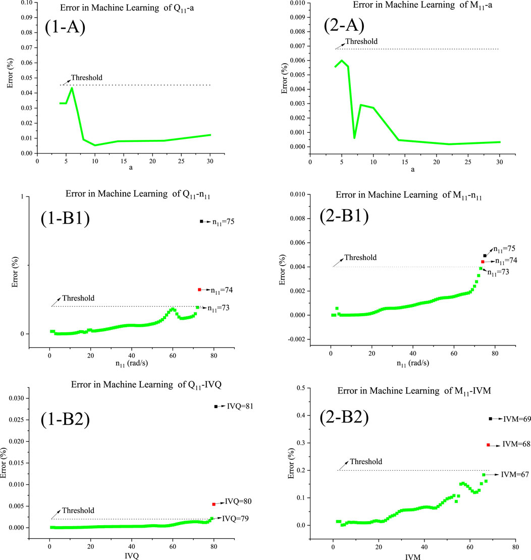
FIGURE 4. ML error. (1-A): $Q_{11}—a$, (1-B1): $Q_{11}—n_{11}$, (1-B2): $Q_{11}—IVQ$, (2-A): $M_{11}—a$, (2-B1): $M_{11}—n_{11}$, and (2-B2): $M_{11}—IVM$.

We use the observation function set given in Eq. 23 to analyze the relationship between $Q_{11}$ and $n_{11}$ based on the relationship between the flow rate and the pump turbine speed.

$O\left(Q_{11}\right)=\left[Q_{11}\right].(23)$

The ML parameter N is determined using the algorithmic flow shown in Figure 2. In actual operation, we continue to increase the value of N and calculate the error as shown in Eq. 19. When this error increases significantly, the prediction model does not match reality. The error at this point is the threshold. We use this N as the boundary of the segmented model. The technical details are as follows:

As $n_{11}$ changes, the linear relationship obtained using the proposed ML algorithm in high-dimensional space is as follows.

• The error corresponding to $n_{11}\ge 0$ is depicted in Figure 4 (1-B1). The ML parameter N (which is $n_{11}$) is set to 73. We define the first region of $Q_{11}-n_{11}$ (P1 of $Q_{11}$) as $0\le n_{11}\le 73$.

• When $n_{11}\ge 73$, we introduce an intermediate variable $IVQ$ and use it to find the linear relationship between $Q_{11}$ and $n_{11}$. The expression for $IVQ$ is given in Eq. 24. The error obtained using ML is depicted in Figure 4 (1-B2). The ML parameter N (i.e., $IVQ$) is set to 79. We define the second region of $Q_{11}—n_{11}$ (P2 of $Q_{11}$) as the region where $n_{11}>73$ and $IVQ\le 79$.

$IVQ=\frac{n_{11}}{e^{Q_{11}}}.(24)$

• When $IVQ>79$, we use $M_{11}=0$ as the dividing line because $M_{11}<0$ causes the control to run away. We define the third region of $Q_{11}—n_{11}$ (P3 of $Q_{11}$) as $IVQ>79$ and $M_{11}>0$.

$Q_{11}—\left(a,n_{11}\right).$

Based on the aforementioned three scenarios, the ML algorithm divides the relationship between $Q_{11}$, $a$, and $n_{11}$ into three areas within the available range. The partition map is illustrated in Figure 4A.

The Relationship Between $M_{11}$, $a$, and $n_{11}$

$M_{11}—a.$

Much like $Q_{11}—a$, the observation function set given in Eq. 25 can reduce the error of the proposed ML algorithm. The resulting error is depicted in Figure 4 (2-A). The vane openings corresponding to all ranges fulfill the requirements under this observation function set.

$O\left(M_{11}\right)=\left[M_{11},M_{11}^2\right],(25)$

$M_{11}—n_{11}.$

Based on the relationship between the torque and speed of a pump turbine, the observation function set given in Eq. 26 is used.

$O\left(M_{11}\right)=\left[M_{11},M_{11}^2,M_{11}^3\right].(26)$

Much like the process used in step 1, we use the ML process in Figure 2 to determine the segment boundary. The technical details are as follows:

• The error corresponding to $n_{11}\ge 0$ is depicted in Figure 4 (2-B1). The parameter N (which is $n_{11}$) is set to 73 in the ML algorithm. We define the first region of $M_{11}—n_{11}$ (P1 of $M_{11}$) as $0\le n_{11}\le 73$.

• When $n_{11}\ge 73$, the intermediate variable $IVM$ is introduced; its expression is given in Eq. 27. The error obtained using the ML algorithm is illustrated in Figure 4 (2-B2). The parameter N (which is $IVM$) in the ML algorithm is set to 67. We define the second region of $M_{11}—n_{11}$ (P2 of $M_{11}$) as $n_{11}>73$and $IVM\le 67$.

$IVM=\frac{n_{11}}{e^{M_{11}/M_{11r}}}.(27)$

where $M_{11r}$is the rated value of $M_{11}$ and has a magnitude of 220.7347.

•For $IVM>67$, we define the third region of $M_{11}—n_{11}$ (P3 of $M_{11}$) as $IVM>67$ and $M_{11}>0$.

$M_{11}—\left(a,n_{11}\right).$

The ML algorithm divides the relationship between $M_{11}$, $a$, and $n_{11}$ into three areas within the available range. The partition map is depicted in Figure 5B.

FIGURE 5

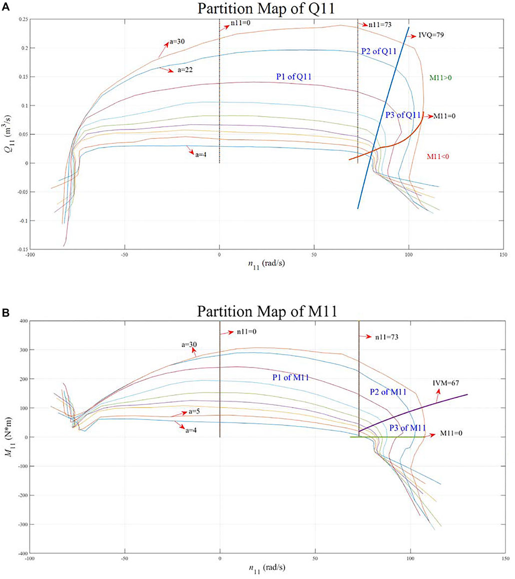
FIGURE 5. Partition maps of (A) $Q_{11}$ and (B) $M_{11}$.

Fit Model

After obtaining the partitions, the principles described in Related Principles are used to establish polynomial models of $Q_{11}$ and $M_{11}$ for each partition as fit models. The polynomial term is the function included in the observation function set. The three-part fit model of $Q_{11}$ is given in Eqs 28–30, and the fitting coefficient values are listed in Table 1. Similarly, the three-part fit model of $M_{11}$ is given in Eqs 31–33, and the fitting coefficients are listed in Table 2.

TABLE 1

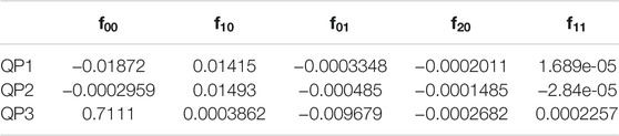
TABLE 1. The $Q_{11}$ fit coefficient values.

TABLE 2

TABLE 2. The $M_{11}$ fit coefficient values.

·P1 of $Q_{11}$

$QP1={\displaystyle \sum _{i=0,j=0}^{i=2,j=1}QP1f_{ij}\cdot a^i\cdot n_{11}^j}=QP1f_{00}+QP1f_{10}\cdot a+QP1f_{01}\cdot n_{11}+QP1f_{20}\cdot a^2+QP1f_{11}\cdot a\cdot n_{11}.(28)$

·P2 of $Q_{11}$

$QP2={\displaystyle \sum _{i=0,j=0}^{i=2,j=1}QP2f_{ij}\cdot a^i\cdot IV{Q}^j}=QP2f_{00}+QP2f_{10}\cdot a+QP2f_{01}\cdot IVQ+QP2f_{20}\cdot a^2+QP2f_{11}\cdot a\cdot IVQ.(29)$

·P3 of $Q_{11}$

$QP3={\displaystyle \sum _{i=0,j=0}^{i=2,j=1}QP3f_{ij}\cdot a^i\cdot n_{11}^j}=QP3f_{00}+QP3f_{10}\cdot a+QP3f_{01}\cdot n_{11}+QP3f_{20}\cdot a^2+QP3f_{11}\cdot a\cdot n_{11}.(30)$

·P1 of $M_{11}$

$\begin{array}{l}MP1={\displaystyle \sum _{i=0,j=0}^{i=2,j=3}MP1f_{ij}\cdot a^i\cdot n_{11}^j}\\ =MP1f_{00}+MP1f_{10}\cdot a+MP1f_{01}\cdot n_{11}+MP1f_{20}\cdot a^2+MP1f_{11}\cdot a\cdot n_{11}+MP1f_{02}\cdot n_{11}^2+MP1f_{21}\cdot a^2\cdot n_{11}+MP1f_{12}\cdot a\cdot n_{11}^2+MP1f_{03}\cdot n_{11}^3.\end{array}(31)$

·P2 of $M_{11}$

$\begin{array}{l}MP2={\displaystyle \sum _{i=0,j=0}^{i=2,j=3}MP2f_{ij}\cdot a^i\cdot n_{11}^j}\\ =MP2f_{00}+MP2f_{10}\cdot a+MP2f_{01}\cdot IVM+MP2f_{20}\cdot a^2+MP2f_{11}\cdot a\cdot IVM+MP2f_{02}\cdot IV{M}^2+MP2f_{21}\cdot a^2\cdot IVM+MP2f_{12}\cdot a\cdot IV{M}^2+MP2f_{03}\cdot IV{M}^3.\end{array}(32)$

·P3 of $M_{11}$

$\begin{array}{l}MP3={\displaystyle \sum _{i=0,j=0}^{i=2,j=3}MP3f_{ij}\cdot a^i\cdot n_{11}^j}\\ =MP3f_{00}+MP3f_{10}\cdot a+MP3f_{01}\cdot n_{11}+MP3f_{20}\cdot a^2+MP3f_{11}\cdot a\cdot n_{11}+MP3f_{02}\cdot n_{11}^2+MP3f_{21}\cdot a^2\cdot n_{11}+MP3f_{12}\cdot a\cdot n_{11}^2+MP3f_{03}\cdot n_{11}^3.\end{array}(33)$

Comprehensive Area Model

Notably, the partition model is chosen because the device model includes multiple expressions, each of which is divided into multiple segments. Since these segments are related directly to differences and coverage, we divide them into multiple regions so that they can accurately represent the device model in a detailed manner. Herein, the partitions $M_{11}$ and $Q_{11}$ are staggered overlapping partitions. Furthermore, we combine the partitions $M_{11}$ and $Q_{11}$ to obtain the comprehensive area, as illustrated in Figure 6. The boundaries in the figure are the parameters in the relationship between the variables determined by the ML algorithm.

FIGURE 6

FIGURE 6. Comprehensive area map.

· Area 1

Condition: $M_{11}>0$, $n_{11}\le 73$, $IVM\le 67$.

Model: $Q_{11}=QP1$, $M_{11}=MP1$.

· Area 2

Condition: $M_{11}>0$, $n_{11}>73$, $IVM\le 67$, $a\le a\ast$.

Model: $Q_{11}=QP2$, $M_{11}=MP2$.

· Area 3

Condition: $M_{11}>0$, $n_{11}>73$, $IVM>67$, $a\le a\ast$.

Model: $Q_{11}=QP2$, $M_{11}=MP3$.

· Area 4

Condition: $M_{11}>0$, $n_{11}>73$, $IVQ\le 79$, $a>a\ast$.

Model: $Q_{11}=QP2$, $M_{11}=MP2$.

· Area 5

Condition: $M_{11}>0$, $n_{11}>73$, $IVQ\le 79$, $IVM\le 67$.

Model: $Q_{11}=QP3$, $M_{11}=MP2$.

· Area 6

Condition: $M_{11}>0$, $n_{11}>73$, $IVQ>79$, $IVM>67$.

Model: $Q_{11}=QP3$, $M_{11}=MP3$.

Other Models

In the description of the pump turbine model, it is necessary to point out the relationship between unit and non-unit quantities, which is expressed using Eqs 34–36.

$n_{11}=n\cdot D/\sqrt{h},(34)$

$Q_{11}=Q/D^2/\sqrt{h},(35)$

$M_{11}=M/D^3/\sqrt{h},(36)$

where $D$ is the nominal diameter of the pump turbine.

Servo Mechanism Model

The servo mechanism model is nonlinear; it considers the speed limit, position limit, position saturation limit, and suppression governor, as depicted in Figure 7. In this model, $\delta$ is the valve stroke, $T_{aB}$ is the auxiliary servomotor response time constant, $T_a$ is the servomotor response time constant, ${\delta }_{\max }$ is the valve stroke upper limit, ${\delta }_{\min }$ is the valve stroke lower limit, $a_{\max }$ is the servomotor stroke upper limit, and $a_{\min }$ is the servomotor stroke lower limit.

FIGURE 7

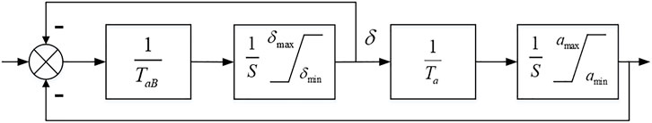
FIGURE 7. Block diagram of the servo mechanism.

Penstock System Model

The approximate elastic water hammer model is used to model the penstock system. Its expression is given in Eq. 37.

$h\left(s\right)=Q\left(s\right)\cdot \frac{-T_{w}s}{0.125T_r^2{s}^2+h_f{T}_{r}s+1},(37)$

where $h\left(s\right)=\mathrm{ℒ}\left\{h\right\}$ and $Q\left(s\right)=\mathrm{ℒ}\left\{Q\right\}$ represent the Laplace transforms of $h$ and $Q$, respectively. $T_w$ is the water inertia time constant, $T_r$ is the water hammer pressure reflection time, and $h_f$ is the head loss coefficient.

Motion Equation Model

When the generator is connected to the pump turbine, the torque of the turbine and the load torque generated by the generator must satisfy the motion equation (Eq. 38).

$M\left(S\right)-M_L\left(S\right)=S\cdot \left(n\left(s\right)\cdot 2B\right),(38)$

where $M\left(s\right)=\mathrm{ℒ}\left\{M\right\}$ and $M_L\left(s\right)=\mathrm{ℒ}\left\{M_L\right\}$ represent the Laplace transforms of $M$ and $M_L$, respectively. $B$ is the inertia time constant of the generator.

MPC Process

Model Prediction

After obtaining the model by using the method introduced in the preceding section, we can predict the value of the state variable. The process is depicted in Figure 8. The details of each module are introduced as follows.

1. Calculate the model calculation value $s\left(k\right)$ at time k using the equipment model.

2. Subtract the model-calculated value $s\left(k\right)$ from the real value $s^{real}\left(k\right)$ at time k to obtain the deviation value $\Delta s\left(k\right)$. The true value comes from the data acquisition component.

3. Calculate the model calculation value $s\left(k+1\right)$ at time k+1 using the equipment model.

4. Add the deviation value $\Delta s\left(k\right)$ at time k and the calculated value $s\left(k+1\right)$ of the model to obtain the predicted value $\widehat{s}\left(k+1\right)$ at time k+1.

5. Calculate the error $error\left(k+1\right)$ between the predicted value $\widehat{s}\left(k+1\right)$ and the real value $s^{real}\left(k+1\right)$ at k+1.

6. Judge whether the error is lower than the limit. If the error is lower than the limit, the prediction level meets the requirements and the prediction model is obtained directly. If the error exceeds the limit, return to step 2 and continue the model prediction process.

FIGURE 8

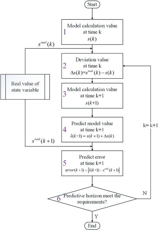
FIGURE 8. Model prediction flowchart.

The predicted values of each of the PSS variables are as follows. Prediction using the pump turbine model:

$\{\begin{array}{l}{\widehat{Q}}_{11}\left(k+1\right)=f_{Q_{11}}\left(\widehat{a}\left(k+1\right),{\widehat{n}}_{11}\left(k+1\right)\right)=Q_{11}\left(k+1\right)+\Delta Q_{11}\left(k\right)\\ \Delta Q_{11}\left(k\right)=Q_{11}^{real}\left(k\right)-Q_{11}\left(k\right)\end{array},(39)$

$\{\begin{array}{l}{\widehat{M}}_{11}\left(k+1\right)=f_{M_{11}}\left(\widehat{a}\left(k+1\right),{\widehat{n}}_{11}\left(k+1\right)\right)=M_{11}\left(k+1\right)+\Delta M_{11}\left(k\right)\\ \Delta M_{11}\left(k\right){=\text{M}}_{11}^{real}\left(k\right)-M_{11}\left(k\right)\end{array}.(40)$

Prediction using the conversion relationship between unit and non-unit quantities:

${\widehat{n}}_{11}\left(k+1\right)=\widehat{n}\left(k+1\right)\cdot D/\sqrt{\widehat{h}\left(k+1\right)},(41)$

${\widehat{Q}}_{11}\left(k+1\right)=\widehat{Q}\left(k+1\right)/D^2/\sqrt{\widehat{h}\left(k+1\right)},(42)$

${\widehat{M}}_{11}\left(k+1\right)=\widehat{M}\left(k+1\right)/D^3/\sqrt{\widehat{h}\left(k+1\right)}.(43)$

Prediction obtained using the penstock system model:

$\{\begin{array}{l}\widehat{h}\left(k+1\right)=f_h\left({\widehat{Q}}_{11}\left(k+1\right)\right)=h\left(k+1\right)+\Delta h\left(k\right)\\ \Delta h\left(k\right)=h^{real}\left(k\right)-h\left(k\right)\end{array}.(44)$

Prediction using the motion equation model:

$\{\begin{array}{l}{\widehat{n}}_{11}\left(k+1\right)=f_{n_{11}}\left({\widehat{M}}_{11}\left(k+1\right),{\widehat{M}}_L\left(K+1\right)\right)=n_{11}\left(k+1\right)+\Delta n_{11}\left(k\right)\\ \Delta n_{11}\left(k\right)=n_{11}^{real}\left(k\right)-n_{11}\left(k\right)\end{array}.(45)$

Optimizer

In this study, we use optimization algorithms as the MPC strategy. The corresponding set of state variables is given in Eq. 46.

$\begin{array}{c}\mathrm{X}=\left\{x_1,x_2,x_3,x_4,x_5\right\}\\ =\left\{\widehat{a}\left(k+1\right),{\widehat{n}}_{11}\left(k+1\right),{\widehat{Q}}_{11}\left(k+1\right),{\widehat{M}}_{11}\left(k+1\right),\widehat{h}\left(k+1\right)\right\}\end{array}.(46)$

The goal of PSS control is to regulate the vane opening such that the turbine operates at the required speed and the system achieves the highest efficiency. Therefore, the objective function is the reciprocal of the turbine efficiency, as shown in Eq. 47.

$J=\underset{X}{\min }\left\{f\left(\mathrm{X}\right)={\widehat{Q}}_{11}\left(k+1\right)\ast \widehat{h}\left(k+1\right)/{\widehat{M}}_{11}\left(k+1\right)\right\}.(47)$

The optimization constraints include equality and inequality constraints. The equality constraints are represented by the model predictions established in Eqs 39–45. The inequality constraints include the upper and lower limits of each state variable, as described in Eqs 48–52.

${\widehat{a}}_{\min }\left(k+1\right)\le \widehat{a}\left(k+1\right)\le {\widehat{a}}_{\max }\left(k+1\right),(48)$

${\widehat{n}}_{11\min }\left(k+1\right)\le {\widehat{n}}_{11}\left(k+1\right)\le {\widehat{n}}_{11\max }\left(k+1\right),(49)$

${\widehat{Q}}_{11\min }\left(k+1\right)\le {\widehat{Q}}_{11}\left(k+1\right)\le {\widehat{Q}}_{11\max }\left(k+1\right),(50)$

${\widehat{M}}_{11\min }\left(k+1\right)\le {\widehat{M}}_{11}\left(k+1\right)\le {\widehat{M}}_{11\max }\left(k+1\right),(51)$

$h_{\min }\left(k+1\right)\le h\left(k+1\right)\le h_{\max }\left(k+1\right).(52)$

The optimization process uses the interior point algorithm, which works well in practice. It has been proven that in some cases, this method can solve a problem to a specified accuracy by performing operations on various polynomials that do not exceed the dimension of the problem.

Numerical Experiments and Analysis

To verify the effectiveness of MPC, we measured and collected data from a PSS in China and conducted simulation experiments using the MATLAB software environment (Mathworks, 2017). The experiment proceeded in three parts, each of which corresponded to no-load start up, frequency disturbance, or speed disturbance. The experiment was performed under medium and low water heads because the PSS easily enters the S-characteristic area under these head levels. We set the water head $h$ to 413 and 418 m and the no-load opening to 0.5. In addition, we used a PSS PID control scheme that was proposed in a previous study for comparison.

No-Load Start-Up Condition

In this part of the experiment, the PSS was in the no-load condition and the pump turbine was started from a standstill. MPC and PID control were implemented when the startup speed reached 90% of the rated speed. The experiment was performed for 120 cycles, each of which ran for approximately 0.2 s. The speed results are depicted in Figure 9. The pump turbine state variable results are depicted in Figure 10. The results indicate that MPC performs better than PID control of PSSs because MPC provides a smaller overshoot and faster response speed.

FIGURE 9

FIGURE 9. Speed variation during no-load start-up under 413 and 418 m of water head.

FIGURE 10

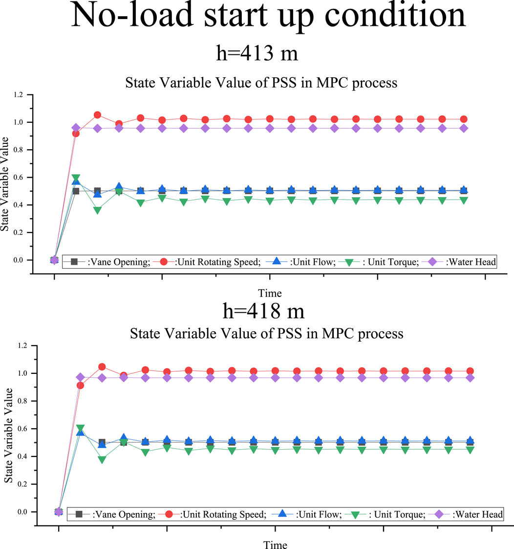
FIGURE 10. PSS MPC state variables during no-load start-up under 413 and 418 m of water head.

Frequency Disturbance Condition

In this part of the experiment, the PSS was operated under no load. For the system frequency to be disturbed at the 10th cycle, the PSS speed needed to be increased to 1.02 times the rated speed. The experimental results obtained under MPC and PID control are depicted in Figure 11 and Figure 12. Both control methods can fulfill the frequency disturbance requirements. Under PID control, the speed overshoots the threshold and the response time is longer. In contrast, the speed overshoot is smaller and the new speed requirements are reached quickly under MPC control.

FIGURE 11

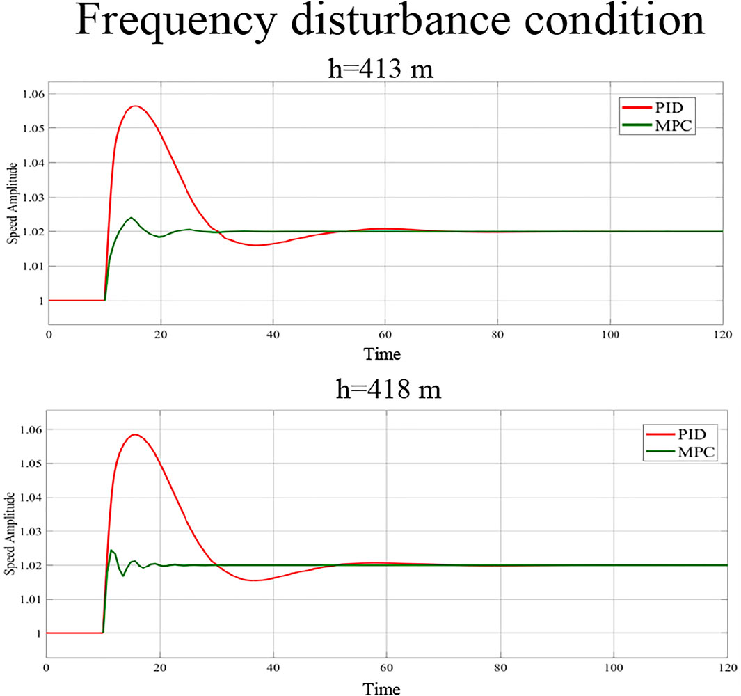
FIGURE 11. Speed variation in the presence of a frequency disturbance under 413 and 418 m of water head.

FIGURE 12

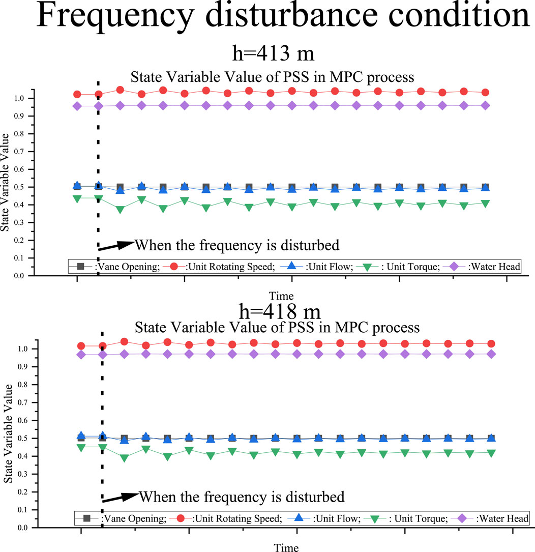
FIGURE 12. PSS MPC state variables in the presence of a frequency disturbance under 413 and 418 m of water head.

Speed Disturbance Condition

In this part of the experiment, the load generator was activated at the 10th cycle and the load torque was increased in steps. At this point, the speed of the pump turbine was disturbed such that it decreased abruptly. The experimental results obtained under MPC and PID control are depicted in Figure 13 and Figure 14. Under PID control, the speed is disturbed in the S-characteristic region. This produces strong oscillation and the speed takes substantial time to stabilize. In contrast, the speed oscillation amplitude is smaller and the speed stabilizes within a short time under MPC control.

FIGURE 13

FIGURE 13. Speed variation due to a speed disturbance under 413 and 418 m of water head.

FIGURE 14

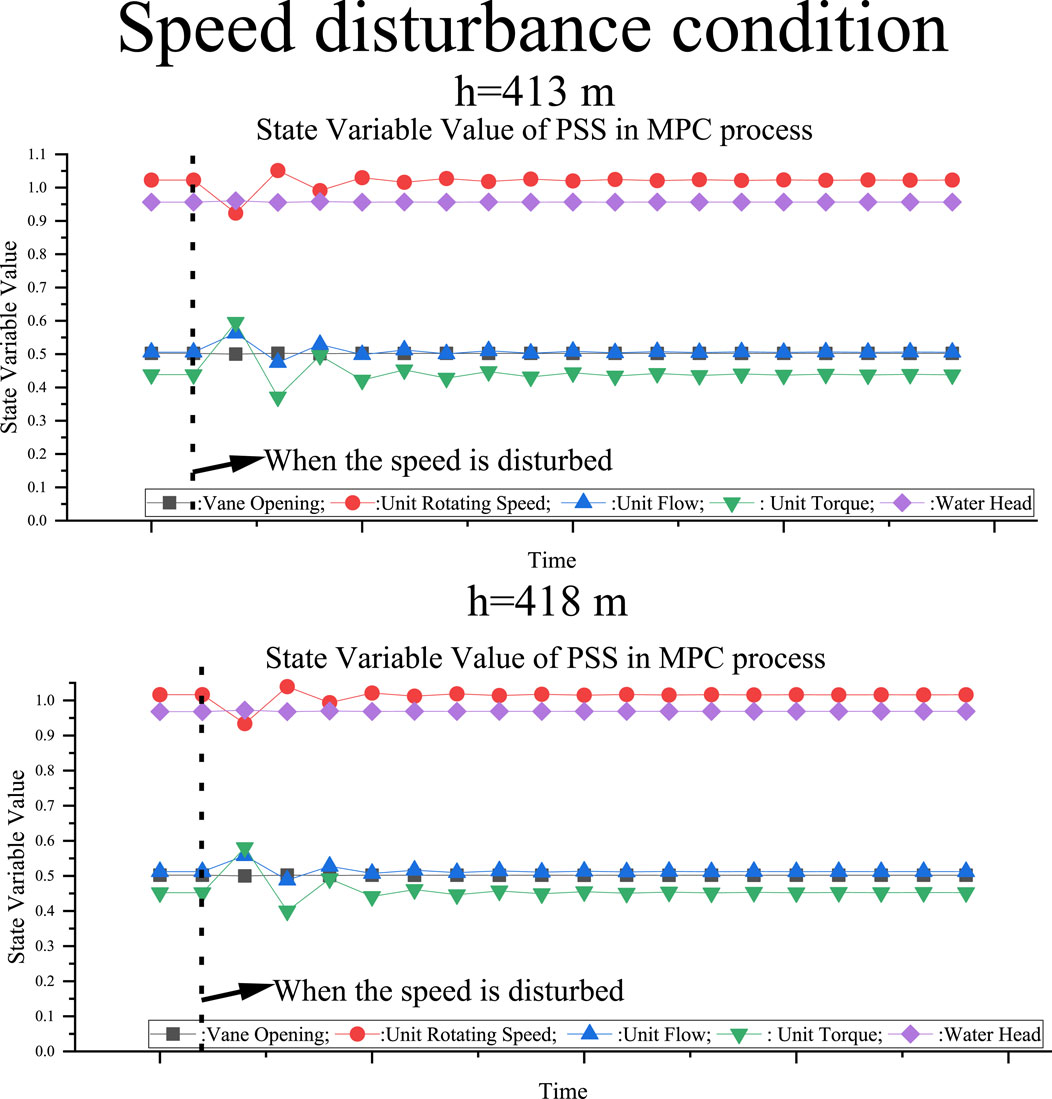
FIGURE 14. PSS MPC state variables in the presence of speed disturbances under 413 and 418 m of water head.

Advantages of MPC

The results described in the preceding section indicate that the MPC and PID control methods can fulfill PSS S-characteristic area control requirements that are otherwise difficult to meet. However, the MPC method offers the following advantages:

• The MPC method can achieve effective control under the conditions of no-load start-up, frequency disturbance, and speed disturbance.

• The model built using ML can accurately represent the PSS. The control program calculation time can be reduced because the established model is simple.

• Since the MPC method uses a global optimization algorithm, the optimal solution within the partition can be calculated directly. Therefore, PSS oscillation in the S feature area can be reduced effectively.

• Under the MPC method, the change of state variable is gentle. Thus, it is substantially conducive to reducing PSS equipment loss.

Conclusion

We proposed an MPC method for PSSs. A ML algorithm based on the Koopman theory was proposed for PSS modeling. A partition model of the pump turbine used in PSSs was established. This allowed us to express the complex nonlinearity of the S-characteristic region using a simple polynomial model. The experimental results indicated that the MPC method quickly reached the control target under conditions of no-load start-up, frequency disturbance, and speed disturbance. This method can more effectively suppress oscillation of the turbine rotation speed in the S-characteristic region than existing control methods and has a faster response speed. The proposed method has practical promise because it learns device characteristics from experimental data and is not limited by device type. In the future, we will improve the accuracy of ML to improve the effect of MPC and study the performance of the proposed method under other working conditions.

Data Availability Statement

The datasets presented in this article are not readily available because Data set for pumped storage system. Requests to access the datasets should be directed to oddnewlife@126.com.

Author Contributions

QC and XL; methodology, QC; software, QC and SY; validation, XL; data curation, PZ; writing—original draft preparation, SY; writing—review and editing, QC; visualization, CG; supervision, XL; project administration, XL; All authors have read and agreed to the published version of the manuscript.

Conflict of Interest

The authors declare that the research was conducted in the absence of any commercial or financial relationships that could be construed as a potential conflict of interest.

Publisher’s Note

All claims expressed in this article are solely those of the authors and do not necessarily represent those of their affiliated organizations, or those of the publisher, the editors and the reviewers. Any product that may be evaluated in this article, or claim that may be made by its manufacturer, is not guaranteed or endorsed by the publisher.

References

Alamir, M., and Allgöwer, F. (2008). Model Predictive Control. Int. J. Robust Nonlinear Control. 18, 799. doi:10.1002/rnc.1266

CrossRef Full Text | Google Scholar

Albuyeh, A. I. F. (2013). Grid of the Future. IEEE Power Energ. Mag. 11 (4), 20. doi:10.1109/MPE.2008.931384

CrossRef Full Text | Google Scholar

Anilkumar, T. T., and Padhy, N. P. (2017). Residential Electricity Cost Minimization Model through Open Well-Pico Turbine Pumped Storage System. Appl. Energ. 195, 23–35. doi:10.1016/j.apenergy.2017.03.020

CrossRef Full Text | Google Scholar

Ayush Thada, S. P., Dubey, A., and Bhaskara Rao, L. (2021). Machine Learning Based Frequency Modelling. Mech. Syst. Signal Process. 160, 107951. doi:10.1016/j.ymssp.2021.107915

CrossRef Full Text | Google Scholar

Bozchalui, M. C. (2015). Optimal Energy Management of Greenhouses in Smart Grids. IEEE TRANSACTIONS SMART GRID 6 (2), 827–835. doi:10.1109/tsg.2014.2372812

CrossRef Full Text | Google Scholar

Brahman, F. H. M., and Jadid, S. (2015). Optimal Electrical and thermal Energy Management of a Residential Energy Hub, Integrating Demand Response and Energy Storage System. Amsterdam: Elsevier. doi:10.1016/j.enbuild.2014.12.039

CrossRef Full Text | Google Scholar

Chen Feng, C. L., Chang, Li., Mai, Z., and Wu, C. (2021). Nonlinear Model Predictive Control for Pumped Storage Plants Based on Online Sequential Extreme Learning Machine with Forgetting FactorComplexity. doi:10.1155/2021/5692621

CrossRef Full Text | Google Scholar

Chunyang Gao, X., Nan, Hg., Men, C., and Fu, J. (2021a). Stability and Dynamic Analysis of Doubly-Fed Variable Speed Pump Turbine Governing System Based on Hopf Bifurcation Theory. Renew. Energ. 175, 568–579.

CrossRef Full Text | Google Scholar

Chunyang Gao, X. Y., Nan, H., Men, C., and Fu, J. (2021b). A Fast High-Precision Model of the Doubly-Fed Pumped Storage Unit. New York, NY: Journal of Electrical Engineering & Technology, 16, 797–808. doi:10.1007/s42835-020-00641-0

CrossRef Full Text | Google Scholar

De Souza, G., and Zanin, A. C. (2010). Real Time Optimization (RTO) with Model Predictive Control (MPC). Comput. Chem. Eng. 34 (12), 1999–2006. doi:10.1016/j.compchemeng.2010.07.001

CrossRef Full Text | Google Scholar

Diego, S., and Carrasco, G. C. G. (2011). Feedforward Model Predictive Control. Annu. Rev. Control. 35, 199–206. doi:10.1016/j.arcontrol.2011.10.007

CrossRef Full Text | Google Scholar

Elena Smirnova, S. K., Kolpak, E., and Shestak, V. (2021). Governmental Support and Renewable Energy Production: A Crosscountry Review. Energy 230. doi:10.1016/j.energy.2021.120903

CrossRef Full Text | Google Scholar

Eric O’Shaughnessy, J. H., Shah, C., and Koebrich, S. (2021). Corporate Acceleration of the Renewable Energy Transition and Implications for Electric Grids. Renew. Sust. Energ. Rev. 146, 111160. doi:10.1016/j.rser.2021.111160

CrossRef Full Text | Google Scholar

Forbes, M. G., Patwardhan, R. S., Hamadah, H., and Gopaluni, R. B. (2015). Model Predictive Control in Industry: Challenges and Opportunities. IFAC-PapersOnLine 48 (8), 531–538. doi:10.1016/j.ifacol.2015.09.022

CrossRef Full Text | Google Scholar

Francesco Calise, M. D. d. A., and Piacentino, A. (2014). A Novel Solar Trigeneration System Integrating PVT (Photovoltaic/thermal Collectors) and SW (Seawater) Desalination. Amsterdam: Dynamic simulation and economic assessment. Energy 67, 129–148. doi:10.1016/j.energy.2013.12.060

CrossRef Full Text | Google Scholar

Güney, T. (2019). Renewable Energy, Non-renewable Energy and Sustainable Development. Int. J. Sust. Develop. World Ecol.. doi:10.1080/13504509.2019.1595214

CrossRef Full Text | Google Scholar

Guopeng Zhao, Y. Z., and Ren, J. (2021). Analysis of Control Characteristics and Design of Control System Based on Internal Parameters in Doubly Fed Variable-Speed Pumped Storage Unit. New Jersey, NY: Complexity. doi:10.1155/2021/6697311

CrossRef Full Text | Google Scholar

Gurung, A. B., Borsdorf, A., Füreder, L., Kienast, F., Matt, P., Scheidegger, C., et al. (2016). Rethinking Pumped Storage Hydropower in the European Alps. Mountain Res. Develop. 36 (2), 222–232. doi:10.1659/mrd-journal-d-15-00069.1

CrossRef Full Text | Google Scholar

Hasan Mehrjerdi, A. A. M. A. (2021). Modeling and Optimal Planning of an Energy–Water–Carbon Nexus System for Sustainable Development of Local CommunitiesAdvanced Sustainable Systems.

Google Scholar

Hou, C. L., Tian, Z., Xu, Ye., Lai, X., Zhang, N., Zheng, T., et al. (2018). Multi-Objective Optimization of Start-Up Strategy for Pumped Storage Units. Energies 1 (5), 1141. doi:10.3390/en11051141

CrossRef Full Text | Google Scholar

Hou, J., Li, W., Guo, W., and Fu, W. (2019). Optimal Successive Start-Up Strategy of Two Hydraulic Coupling Pumped Storage Units Based on Multi-Objective Control. Int. J. Electr. Power Energ. Syst. 111, 398–410. doi:10.1016/j.ijepes.2019.04.033

CrossRef Full Text | Google Scholar

Huang, W., Guo, X., Wang, J., Li, J., and Li, J. (2018). Prediction Method for the Complete Characteristic Curves of a Francis Pump-Turbine. Water 10 (2), 205. doi:10.3390/w10020205

CrossRef Full Text | Google Scholar

Idowu, S., Saguna, S., Åhlund, C., and Schelén, O. (2016). Applied Machine Learning: Forecasting Heat Load in District Heating System. Energy and Buildings 133, 478–488. doi:10.1016/j.enbuild.2016.09.068

CrossRef Full Text | Google Scholar

Jianzhong Zhou, Z. Z., Zhang, Chu., Li, C., and Xu, Y. (2018). A Real-Time Accurate Model and its Predictive Fuzzy PID Controller for Pumped Storage Unit via Error Compensation. Energies 11 (1), 35. doi:10.3390/en11010035

CrossRef Full Text | Google Scholar

Julian David Hunt, B. Z., Rafael Lopes, P. S. Fo. B., and Andreas, N. (2020). Existing and New Arrangements of Pumped-Hydro Storage Plants. Renew. Sust. Energ. Rev. 129, 109914. doi:10.1016/j.rser.2020.109914

CrossRef Full Text | Google Scholar

Kiely, T. J., Kiely, N. D. B., and Bastian, N. D. (2019). The Spatially Conscious Machine Learning Model. Stat. Anal. Data Min: ASA Data Sci. J. 13 (1), 31–49. doi:10.1002/sam.11440

CrossRef Full Text | Google Scholar

Kocaman, A. S., and Modi, V. (2017). Value of Pumped Hydro Storage in a Hybrid Energy Generation and Allocation System. Appl. Energ. 205, 1202–1215. doi:10.1016/j.apenergy.2017.08.129

CrossRef Full Text | Google Scholar

Li, C., Mao, Y., Yang, J., and Xu, Y. (2017b). A Nonlinear Generalized Predictive Control for Pumped Storage Unit. Renew. Energ. 114, 945–959. doi:10.1016/j.renene.2017.07.055

CrossRef Full Text | Google Scholar

Li, J.-w., ZhangXian, H-z., Xian, H.-z., and Yu, J.-x. (2017a). Numerical Simulation of Hydraulic Force on the Impeller of Reversible Pump Turbines in Generating Mode. J. Hydrodyn 29, 603–609. doi:10.1016/s1001-6058(16)60773-4

CrossRef Full Text | Google Scholar

Li, J., Ward, J. K., Tong, J., and Platt, G. (2016). Machine Learning for Solar Irradiance Forecasting of Photovoltaic System. Renew. Energ. 90, 542–553. doi:10.1016/j.renene.2015.12.069

CrossRef Full Text | Google Scholar

Liang, L., and Hou, D. J. (2019). GPU-based Enumeration Model Predictive Control of Pumped Storage to Enhance Operational Flexibility. IEEE Trans. Smart Grid 10 (5), 5223–5233. doi:10.1109/tsg.2018.2879226

CrossRef Full Text | Google Scholar

Martin, R., Aler, R., and Galvan, I. M. (2015). Machine Learning Techniques for Daily Solar Energy Prediction and Interpolation Using Numerical Weather Models. Concurrency Computat.: Pract. Exper. 28, 1261–1274. doi:10.1002/cpe.3631

CrossRef Full Text | Google Scholar

Mathworks, MW (2017). Matlabs Optimization Toolbox. [online].

Google Scholar

Max Schwenzer, M. A., Bergs, T., and Abel, D. (2021). Review on Model Predictive Control: an Engineering Perspective. Int. J. Adv. Manufacturing Tech.. doi:10.1007/s00170-021-07682-3

CrossRef Full Text | Google Scholar

Mayne, D. (2016). Robust and Stochastic Model Predictive Control: Are We Going in the Right Direction?. Annu. Rev. Control. 41, 184–192. doi:10.1016/j.arcontrol.2016.04.006

CrossRef Full Text | Google Scholar

Menon, R. P. (2013). Study of Optimal Design of Polygeneration Systems in Optimal Control Strategies. Amsterdam: Energy 55, 134–141. doi:10.1016/j.energy.2013.03.070

CrossRef Full Text | Google Scholar

Min, C.-G., and Kim, M.-K. (2017). Flexibility-Based Reserve Scheduling of Pumped Hydroelectric Energy Storage in Korea. Energies 10 (10), 1478. doi:10.3390/en10101478

CrossRef Full Text | Google Scholar

Olusola Bamisile, A. B., Humphrey, A., Nasser, Y., Mukhtar, M., Huang, Qi., and Hu, W. (2021). Electrification and Renewable Energy Nexus in Developing Countries; an Overarching Analysis of Hydrogen Production and Electric Vehicles Integrality in Renewable Energy Penetration. Energ. Convers. Manage. 235, 114023. doi:10.1016/j.enconman.2021.114023

CrossRef Full Text | Google Scholar

Pan, W., Zhu, Z., Liu, T., and Tian, W. (2021). Optimal Control for Speed Governing System of On-Grid Adjustable-Speed Pumped Storage Unit Aimed at Transient Performance Improvement. IEEE Access 9, 40445–40457. doi:10.1109/access.2021.3063434

CrossRef Full Text | Google Scholar

Pannatier, Y., Kawkabani, B., Nicolet, C., Schwery, A., and Allenbach, P. (2010). Investigation of Control Strategies for Variable-Speed Pump-Turbine Units by Using a Simplified Model of the Converters. IEEE Trans. Ind. Electron. 57, 3039–3049. doi:10.1109/tie.2009.2037101

CrossRef Full Text | Google Scholar

Pazouki, S. H. M.-R. (2016). Optimal Planning and Scheduling of Energy Hub in Presence of Wind, Storage and Demand Response under Uncertainty. Int. J. Electr. Power Energ. Syst. doi:10.1016/j.ijepes.2016.01.044

CrossRef Full Text | Google Scholar

Pazouki, S. (2014). Uncertainty Modeling in Optimal Operation of Energy Hub in Presence of Wind, Storage and Demand Response. Amsterdam: International Journal of Electrical Power and Energy Systems, 61, 33–345. doi:10.1016/j.ijepes.2014.03.038

CrossRef Full Text | Google Scholar

Podlubny, I. (1999). Fractional-order Systems and PI/sup/spl lambda//D/sup/spl Mu//-Controllers. IEEE Trans. Automat. Contr. 44 (1), 208–214. doi:10.1109/9.739144

CrossRef Full Text | Google Scholar

Pradhan, A., and Franca, M. J. (2021). The Adoption of Seawater Pump Storage Hydropower Systems Increases the Share of Renewable Energy Production in Small Island Developing States. Renew. Energ. 177, 448–460. doi:10.1016/j.renene.2021.05.151

CrossRef Full Text | Google Scholar

Rajkumar, R. K. (2011). Techno-economical Optimization of Hybrid Pv/wind/battery System Using Neuro-Fuzzy. Energy 36 (8), 5148–5153. doi:10.1016/j.energy.2011.06.017

CrossRef Full Text | Google Scholar

Rajvikram Madurai Elavarasan, R. P., Jamal, T., Dyduch, Ja., Arif, M. T., Shafiullah, G. M., Chopra, St. S., et al. (2021). Envisioning the UN Sustainable Development Goals (SDGs) through the Lens of Energy Sustainability (SDG 7) in the post-COVID-19 World. Appl. Energ. 292. doi:10.1016/j.apenergy.2021.116665

CrossRef Full Text | Google Scholar

Robinson, C., Dilkina, B., Hubbs, J., Zhang, W., Guhathakurta, S., and Pendyala, R. M. (2017). Machine Learning Approaches for Estimating Commercial Building Energy Consumption. Appl. Energ. 208, 889–904. doi:10.1016/j.apenergy.2017.09.060

CrossRef Full Text | Google Scholar

Ruppert, L., List, B., Bauer, C., and Bauer, C. (2017). An Analysis of Different Pumped Storage Schemes from a Technological and Economic Perspective. Energy 141, 368–379. doi:10.1016/j.energy.2017.09.057

CrossRef Full Text | Google Scholar

Sam, N. K., and Gounden, N. A. (2017). Wind-driven Stand-Alone DFIG with Battery and Pumped Hydro Storage System. Sādhanā 42, 173–185. doi:10.1007/s12046-017-0595-ys

CrossRef Full Text | Google Scholar

Sánchez-Oro, J., and Duarte, A. (2016). Robust Total Energy Demand Estimation with a Hybrid Variable Neighborhood Search - Extreme Learning Machine Algorithm. Energ. Convers. Manage. 123, 445–452. doi:10.1016/j.enconman.2016.06.050

CrossRef Full Text | Google Scholar

Schmidt, J., and Kemmetmüller, W. (2017). Modeling and Static Optimization of a Variable Speed Pumped Storage Power Plant. Renew. Energ. 111, 38–51. doi:10.1016/j.renene.2017.03.055

CrossRef Full Text | Google Scholar

Shiliang Zhang, H. C., Zhang, Y., Jia, L., Ye, Z., and Hei, X. (2017). Data-Driven Optimization Framework for Nonlinear Model Predictive Control. Math. Probl. Eng. 2017, 15. doi:10.1155/2017/9402684

CrossRef Full Text | Google Scholar

Sopasakis, P., and Sarimveis, H. (2017). Stabilising Model Predictive Control for Discrete-Time Fractional-Order Systems. Automatica 75, 24–31. doi:10.1016/j.automatica.2016.09.014

CrossRef Full Text | Google Scholar

Thomas Sattich, D. F., Scholten, D., and Yan, S. (2021). Renewable Energy in EU-China Relations: Policy Interdependence and its Geopolitical Implications. Energy Policy 156, 112456. doi:10.1016/j.enpol.2021.112456

CrossRef Full Text | Google Scholar

van Meerwijk, A. J. H., Davila-martinezBenders, A., and LaugsLAUGS, G. A. H. (2016). Swiss Pumped Hydro Storage Potential for Germany's Electricity System under High Penetration of Intermittent Renewable Energy. J. Mod. Power Syst. Clean. Energ. 4 (4), 542–553. doi:10.1007/s40565-016-0239-y

CrossRef Full Text | Google Scholar

Xu, Y., Zheng, Y., Du, Y., Yang, W., and Li, C. (2018). Adaptive Condition Predictive-Fuzzy PID Optimal Control of Start-Up Process for Pumped Storage Unit at Low Head Area. Energ. Convers. Manage. 177, 592–604. doi:10.1016/j.enconman.2018.10.004

CrossRef Full Text | Google Scholar

Xu, Y., Zhou, J., Xue, X., Fu, W., and Li, C. (2016). An Adaptively Fast Fuzzy Fractional Order PID Control for Pumped Storage Hydro Unit Using Improved Gravitational Search Algorithm. Energ. Convers. Manage. 111, 67–78. doi:10.1016/j.enconman.2015.12.049

CrossRef Full Text | Google Scholar

Ye, B.-L., Wu, W., Gao, H., Lu, Y., and Zhu, L. (2017). Stochastic Model Predictive Control for Urban Traffic Networks. Appl. Sci. 7 (6), 588. doi:10.3390/app7060588

CrossRef Full Text | Google Scholar

Yifeng Shi, X. S., Yi, C., Song, X., and Chen, X. (2020). Control of the Variable-Speed Pumped Storage Unit-Wind Integrated System Mathematical Problems In Engineering 2020. doi:10.1155/2020/3816752

CrossRef Full Text | Google Scholar

Yin, J., Wang, D., and Wei, X. (2014). Investigation of the Unstable Flow Phenomenon in a Pump Turbine. Sci. China Phys. Mech. Astron. 57, 1119–1127. doi:10.1007/s11433-013-5211-5

CrossRef Full Text | Google Scholar

Zeng, W., and Hu, J. (2017). Pumped Storage System Model and Experimental Investigations on S-Induced Issues during Transients. Mech. Syst. Signal Process. 90, 350–364. doi:10.1016/j.ymssp.2016.12.031

CrossRef Full Text | Google Scholar

Zhang, H., Chen, D., Wu, C., Wang, X., Lee, J.-M., and Jung, K.-H. (2017). Dynamic Modeling and Dynamical Analysis of Pump-Turbines in S-Shaped Regions during Runaway Operation. Energ. Convers. Manage. 138, 375–382. doi:10.1016/j.enconman.2017.01.053

CrossRef Full Text | Google Scholar

Zhang, X. S. M., Alabdulwahab, A., and Abusorrah, A. (2015). Optimal Expansion Planning of Energy Hub with Multiple Energy Infrastructures. Smart Grid IEEE Trans. 6 (5), 2302–2311. doi:10.1109/tsg.2015.2390640

CrossRef Full Text | Google Scholar

Zhao, Y.-P., Hu, Q.-K., Xu, J.-G., Li, B., and Pan, Y.-T. (2018). A Robust Extreme Learning Machine for Modeling a Small-Scale Turbojet Engine. Appl. Energ. 218, 22–35. doi:10.1016/j.apenergy.2018.02.175

CrossRef Full Text | Google Scholar

Zhaoyang Dong, J. Z., and Wen, F. (2014). From Smart Grid to Energy Internet: Basic Concept and Research Framework. Automat Elec Power Syst. 38 (15), 1–11.

Google Scholar

Zhigao Zhao, J. Y., Yang, W., Hu, J., and Chen, M. (2019). A Coordinated Optimization Framework for Flexible Operation of Pumped Storage Hydropower System: Nonlinear Modeling, Strategy Optimization and Decision Making. Energ. Convers. Manage. 194, 70–93. doi:10.1016/j.enconman.2019.04.068

CrossRef Full Text | Google Scholar