Can Machine Learning be Applied to Carbon Emissions Analysis: An Application to the CO2 Emissions Analysis Using Gaussian Process Regression

In this paper, a nonparametric kernel prediction algorithm in machine learning is applied to predict CO₂ emissions. A literature review has been conducted so that proper independent variables can be identified. Traditional parametric modeling approaches and the Gaussian Process Regression (GPR) algorithms were introduced, and their prediction performance was summarized. The reliability and efficiency of the proposed algorithms were then demonstrated through the comparison of the actual and the predicted results. The results showed that the GPR method can give the most accurate predictions on CO₂ emissions.

Introduction

As the population of the earth is being exponentially increasing, the exhaustion of carbon dioxide is increasing day by day resulting in the extreme overheating of the environment, which has become a significant reason for climate change. Global efforts to mitigate climate change were focused on the reduction of future days with extreme overheating of the environment. There are many research and surveys that have been conducted by various scientists, students, and other officials which were about the reasons for the high emission of CO₂ in different countries. Most of the empirical studies took the parametric modeling approach to analyze the factors that initiate and support the emission of CO₂. However, the traditional parametric approach optimizes a function to a known form with a set of finite and pre-determined parameters. This rigidity limits the predictive power of the parametric models. In recent years, nonparametric machine learning techniques have played dominantly with the enhancement of the forecast.

In this paper, a Bayesian nonparametric kernel prediction algorithm in machine learning is applied to predict CO₂ emissions. A literature review has been conducted so that the proper independent variables have been identified. Classical least squares, robust least squares, and algorithms of the GPR were introduced and their prediction performance, including the evaluation criteria that are effective in the measurements for model performance, were summarized. The reliability and efficiency of the proposed algorithms were then demonstrated through the comparison between the actual data and the predicted results. It is found that GPR can give the most accurate predictions on CO₂ emissions.

Literature Review

The growth of the economy, energy utilization, and CO₂ emissions are deeply related to each other. Kolstad and Krautkraemer (1993) point out that while the use of resources like the energy has a bright side on growth, it has negative environmental impacts. Traditional growth theories like the Solow growth model failed to consider the environmental impacts of growth (Solow, 1956). More modern growth theories study the interrelationship among energy, the environment, and economic growth (see, for example, Kolstad and Krautkraemer (1993), Jorgenson and Wilcoxen (1993) or Xepapadeas (2005) for a brief review).

Empirical studies depict that the growth of the economy and the ingestion of energy incorporates with the process of CO₂ emission. Recently, Hu et al. (2020) study the dominant reasons for carbon emission among the Belt and Road countries and find that CO₂ emissions have increased significantly due to economic growth. Similarly, Shabaz et al. (2013) found that in Indonesia, the emission of CO₂ increased for the extreme boost of the economic zone, while Shahbaz et al. (2016) found that economic growth led to CO₂ emissions in Bangladesh and Egypt. Meanwhile, other studies discovered a bilateral causal relationship among the three variables. Munir et al. (2020) prove the fact that there is a relation of aftermaths and economy between GDP and energy ingestion in the major countries of the ASEAN (Association of Southeast Asian Nations), while Liu and Hao (2018) find that in energy-exporting countries, there is a bilateral relationship which may be a full-duplex connection between CO₂ emissions, energy utilization, and GDP per capita. Similarly, a repeating loop effect is observed between energy ingestion, CO₂ emission, and the advancement of the economy by Kahouli (2018). Accordingly, Mohmannd et al. (2020) observed the working principle of the causal relationship among transportation infrastructure, economic growth, and transportation emissions from 1971 to 2017 in Pakistan. The results show short-term causality from transportation infrastructure, economic growth, fuel consumption to CO₂ emissions, and the long-run relationship between economic advancement and infrastructure.

Apart from the growth and energy consumption, industrialization, population growth, and income level also contributed a great share in global carbon emissions. Minx et al. (2011) found that “industrialization” can be taken into consideration for the rapid increase of carbon dioxide emission in China from 2002 to 2007 while Zhang et al. (2014) found that the growth of the tertiary industry can decrease the CO₂ exhalation intensity. Nasir et al. (2021) examined the connection between the factors which are the exhalation of CO₂, industrialization, growth of the economy, energy ingestion, and several connecting factors from 1980 to 2014 in Australia. The observations of those involved say that all variables affect CO₂ emissions. Li et al. (2021) discussed the effect of the growth and structure of the economy on per capita CO₂ emissions in 147 countries from 1990 to 2015. The results show that at the global level, economic growth and economic structure are the most significant positive and positive effects, respectively.

Studies on population have thus far concentrated on the relationship between population growth and emission increase. The effect of population growth on CO₂ emissions can be summarized as follows (Birdsall, 1992): On one side, the energy demand was increased for power generation, industry, and transport. On the contrary, it increased deforestation emissions due to population growth. Empirically, Knapp and Mookerjee (1996) conducted a Granger causality test on annual data from 1880 to 1989 to determine the connecting clauses between global population expansion and carbon dioxide exhaustion. The results show there is a short-term dynamic relationship between the exhaustion of carbon dioxide and population growth. Very recently, Zhang et al. (2020) analyzed the knot between CO₂ emissions, GDP, and fuel ingestion in China and ASEAN countries. It was found that carbon density, energy intensity, GDP, and population are positively correlated with CO₂ emissions. Empirical findings also show that the developing countries are facing the effect of overpopulation and that’s why, they are facing more of a carbon emissions record per year other than the developed countries (Shi, 2003).

In the past decade, the theory and methodology of the Environmental Kuznets Curve (EKC) have been used to analyze the relationship between the net income and exhaustion of carbon of an area (Dinda, 2004; Williams and Rasmussen, 1996). According to the EKC, at relatively low-income levels, emissions increase as income increases. After a certain point, emissions will decline with income. Thus, the emission of CO₂ varies concerning the level of income. Luo et al. (2021) investigated the influencing factors of Shanghai’s CO₂ emissions from 1995 to 2017. They found that personal disposable income is one of the top drivers of CO₂ emissions. Yuan et al. (2014) examined the long-term relationship between China’s per capita income, ingestion of energy, and the emission of CO₂ from 1953 to 2008. They found out, there is a unilateral Granger inter-relation between the gross national income and the emission of CO₂.

Based on the literature above, it concludes that economic up-gradation, energy utilization, manpower density, industrialization, and income can be classified as the predominant factors affecting CO₂ emissions. Other factors might also affect CO₂ emissions in China. For example, R&D (Nguyen et al., 2020; Jones, 1995), financial development (Bhattacharya et al., 2017; Zaidi et al., 2019; Wang et al., 2020), the degree of foreign direct investment (Essandoh et al., 2020; Le et al., 2020; Khan and Rana, 2021. etc). This paper limits the focus on how well the different prediction models perform based on the information set which includes only the most predominant driver of CO₂ emissions and excludes those unimportant ones to be captured by the stochastic terms in the models.

Methodology

Gaussian Process Regression (GPR) method can be introduced as a non-parametric Bayesian regression method (Gershman and Blei, 2012). It captures a wide variety of relations between inputs and outputs and lets the data determine the complexity of the underlying functions through the means of Bayesian inference (Williams, 1998). Considering the output$y$ of a function $w$ at input $x$ with independent and identically distributed random noise $\epsilon \sim \mathcal{N}\left(0,{\sigma }_n^2\right)$. The function accompanied with the distributed random noise can be presented as:

$y=w\left(x\right)+\epsilon (1)$

In classical linear regression, $w\left(x\right)$ is deterministic whereas the noise term is random. In Gaussian process regression, however, $w\left(x\right)$ is assumed to be random and follows a Gaussian process. A Gaussian process is an extension of multivariant Gaussian distribution to infinite dimensions; any finite subset sampled from the Gaussian process follows multiple Gaussian distributions (MacKay, 1998). The distribution over functions can be described with the help of the Gaussian process,

$w\left(x\right)=\mathcal{GP}\left(m\left(x\right),k\left(x,x^{\text{'}}\right)\right)(2)$

where $x$ is applied as the input variable, $m\left(x\right)$ is denoted as the mean function, finally, $k\left(x,x^{\text{'}}\right)$ is known as covariance function. These two functions are defined respectively as:$m\left(x\right)=\mathbb{E}\left[w\left(x\right)\right]$

$k\left(x,x^{\text{'}}\right)=cov\left[w\left(x\right),w\left(x^{\text{'}}\right)\right].(3)$

A finite collection of function values sampled from the Gaussian process follows multiple Gaussian distributions:

${\left[w\left(x^{\left(1\right)}\right),w\left(x^{\left(2\right)}\right),\dots ,w\left(x^{\left(n\right)}\right)\right]}^{\text{T}}\sim \mathcal{N}\left(\mathit{\mu },K\right)(4)$

where $K$ is a $n\times n$ (n by n) matrix with the entries $K_{ij}=k\left(x^{\left(i\right)},x^{\left(j\right)}\right)$ and $\mu$ has entries ${\mu }_i=m\left(x^{\left(i\right)}\right)$. Given a training set that contains observation points $\mathit{y}={\left[y\left(x^{\left(1\right)}\right),y\left(x^{\left(2\right)}\right),\dots ,y\left(x^{\left(n\right)}\right)\right]}^{\text{T}}$ and function values $\mathit{w}={\left[w\left(x^{\left(1\right)}\right),w\left(x^{\left(2\right)}\right),\dots ,w\left(x^{\left(n\right)}\right)\right]}^{\text{T}}$, it follows that the conditional distribution $p\left(y|w\right)$ and the Gaussian prior $p\left(w\right)$ are $\mathcal{N}\left(w,{\sigma }_{\epsilon }^{2}I\right)$ and $\mathcal{N}\left(\mu ,K\right)$, respectively. By definition, the set of observations $y$ and the set of function values $w$ follow a joint multivariate Gaussian distribution. The join distribution $p\left(w\left(x^{\ast }\right), y\right)$ is defined as

$\left[\begin{array}{c}w\left(x^{\ast }\right)\\ y\end{array}\right]\sim \mathcal{N}\left(\left[\begin{array}{c}{\mu }^{\ast }\\ \mu \end{array}\right],\left[\begin{array}{cc}k\left(x^{\ast },x^{\ast }\right)& k^{\ast \mathrm{T}}\\ k^{\ast }& K+{\sigma }_{\epsilon }^{2}I\end{array}\right]\right)(5)$

Here, $I$ will be considered as the identity matrix, ${\sigma }_{\epsilon }^2$ is the unknown variance of the random noise and ${\left({\mathit{k}}^{\ast }\right)}_i=k\left(x^{\ast },x^{\left(i\right)}\right)$ for $i=\mathrm{1,2},\dots ,N$. Using the Bayesian rule, the predictive posterior, $p\left(w\left(x^{\ast }\right)\text{|}\mathit{y}\right)\sim \mathcal{N}\left({\overline{w}}^{\ast },{\text{Σ}}^{\ast }\right)$, can be obtained, and the mean ${\overline{w}}^{\ast }$and variance ${\text{Σ}}^{\ast }$ are defined by

${\overline{w}}^{\ast }={\mu }^{\ast }+{\left(k^{\ast }\right)}^T{\left[K+{\sigma }_{\epsilon }^{2}I\right]}^{-1}\left(y-\mu \right){\Sigma }^{\ast }=k\left(x^{\ast },x^{\ast }\right)-{\left(k^{\ast }\right)}^T{\left[K+{\sigma }_{\epsilon }^{2}I\right]}^{-1}\left(k^{\ast }\right)(6)$

The covariance function determines the characteristics of the Gaussian method that can be expressed as $k\left(x^{\left(i\right)},x^{\left(j\right)}\right)$. The covariance function models the dependence between the function values at different input points $x^{\left(i\right)}$ and $x^{\left(j\right)}$. The covariance function is often called the kernel of the Gaussian process. There are many possible options for the prior covariance function. A popular kernel is the exponential covariance function which allows the model to general a non-negative definite covariance matrix for any set of input points (Williams and Rasmussen, 1996). The exponential covariance function is defined as

$k\left(x^{\left(i\right)},x^{\left(j\right)}\right)={\sigma }_f^{2}exp\left(-\frac{\parallel x^{\left(i\right)}-x^{\left(j\right)}{\parallel }^2}{2I^2}\right)+{\sigma }_{\epsilon }^2{\delta }_{ij}(7)$

where $\mathit{I}$ is the characteristic length scale, ${\sigma }_f^2$ is the signal variance, and ${\delta }_{ij}$ is a Kronecker delta. The Gaussian process regression employs a set of hyperparameters $\theta$ including $I$, ${\sigma }_f^2$ and ${\sigma }_n^2$ to increase or reduce the priority correlation between points and consequentially the variability of the resulting function. The hyperparameters $\theta$ can be optimized based on the log-likelihood framework:

$L=\log p\left(y|w,\theta \right)=-\frac{1}{2} y^T{C}^{-1}y-\frac{1}{2}\log \left|C\right|-\frac{n}{2}\log 2\pi , C=K+{\sigma }_{\epsilon }^{2}I(8)$

More details about the regression process of Gaussian can be researched and acknowledged in the book of Williams and Rasmussen (2006), available free online and is accessible via the link: www.GaussianProcess.org/gpml.

Empirical Results

A literature review has been conducted so that five independent variables; namely: economic growth, energy consumption, population, industrialization, and income, have been identified. In this study, the GPR method and the other proposed algorithms are applied to study carbon emissions in China. Economic growth is approximated by GDP (100 million RMB), energy consumption is approximated by per capita energy consumption (tons of standard coal), the population is approximated by population size (10,000 people), industrialization is weighted by the percentage of secondary industry in China, and income is measure by the average annual salary (RMB).

The data of GDP, population size, energy consumption, percentage of secondary industry, and average annual salary are collected from the China City Statistical Yearbook. CO₂ emissions data come from four main sources of energy consumption. These are electricity, fuel, heating, and transportation. Those data can be obtained and calculated through the China Urban Construction Statistical Yearbook, the China City Statistical Yearbook, and the submerged government Panel on the change of weather and climate. Since some of those data is not available after 2014, the data in this paper range from the year 2002–2014.

Statistical Analysis of Prediction Results

The commonly used criteria in prediction performance are used in this study to evaluate the validity of the fitting. In Table 1, the root means squared error (RMSE), the mean squared error (MSE), the R-square, and the mean absolute error (MSE) are shown, where a well-fitted model should have R-square close to 1, whereas the RMSE, the MSE, and the MAE should be as small as possible. As per the observation from Table 1, Exponential GPR provides the best fit data as it has the smallest RMSE, MSE, and MAE, and an R-square closest to 1.

TABLE 1

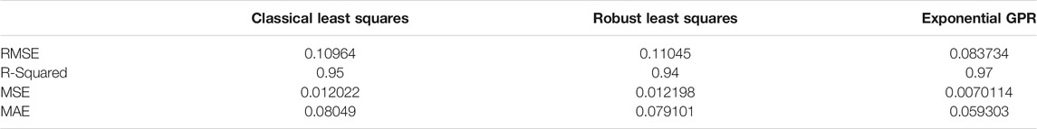
TABLE 1. Statistical Analysis of Prediction Results.

Data Visualization

Since the data set is large, which made it difficult to demonstrate and view the whole set of data, visualization methods are typically needed especially for representative scenarios. The prediction results were analyzed at the model level to see the allover authenticity of the three models and at the individual component level to get a picture of the estimates produced by the three models over the range of some particular variable.

At the overall level, the comparison and deviation of the actual value and the predicted dimension of the emission of carbon dioxide are determined. Figure 1 demonstrates the comparison of actual value and prediction of CO₂ emissions predicted by the three models; for each model, the predicted value is plotted against the actual value. To have a good fit, each plot should resemble a straight line at 45°. However, compare with the exponential GPR model, for the classical least squares model and the robust least-squares model, the predicted values are larger than the actual values over the range of 3.5–4 logarithm units of CO₂ emissions. This means that the classical least squares model and the robust least-squares model are overestimating CO₂ emissions over a particular range compare with the exponential GPR model. The same issue can be observed from Figure 2 which shows the deviation of actual value and prediction of CO₂ emissions for the three models. Figure 2 shows that, compare with the other two models, the deviations for the exponential GPR model cluster more closely around the horizontal line which represents no deviations. It suggests that the exponential GPR model provides a much better fit than the other two models.

FIGURE 1

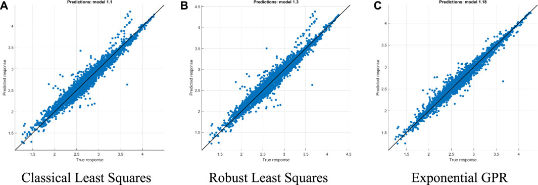
FIGURE 1. Comparison of actual value and prediction of CO₂ emissions between the selected models. (A) Classical Least Squares. (B) Robust Least Squares. (C) Exponential GPR. Notes: 1) The horizontal axis represents actual CO₂ emissions in logarithm, and the vertical axis represents predicted CO₂ emissions in logarithm. 2) CO₂ emissions are measured in ten thousand tons of standard coal.

FIGURE 2

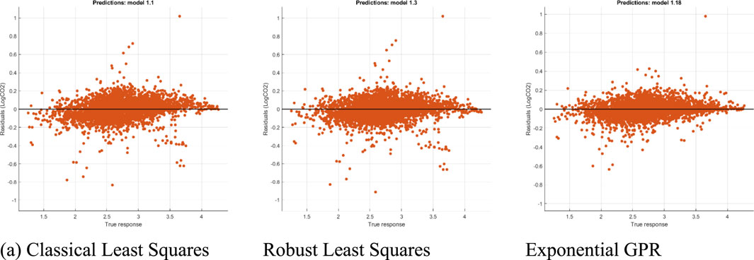
FIGURE 2. The deviation of actual value and prediction of CO₂ emissions between the selected models. (A) Classical Least Squares, Robust Least Squares, Exponential GPR. Notes: 1) The horizontal axis represents actual CO₂ emissions in logarithm, and the deviation of the actual extremity of the CO₂ emission from the predicted value is represented by the vertical axis. 2) CO₂ emissions are measured in ten thousand tons of

Apart from analyzing the prediction results at the overall model level, the all over performance of the three models is also be evaluated at an individual component level. At the individual component level, the estimates produced by the selected models are analyzed over the extended range of some particular variables. Figures 3–7 below plot the actual and predicted values of CO₂ emissions against each of the most predominant factors of the models.

FIGURE 3

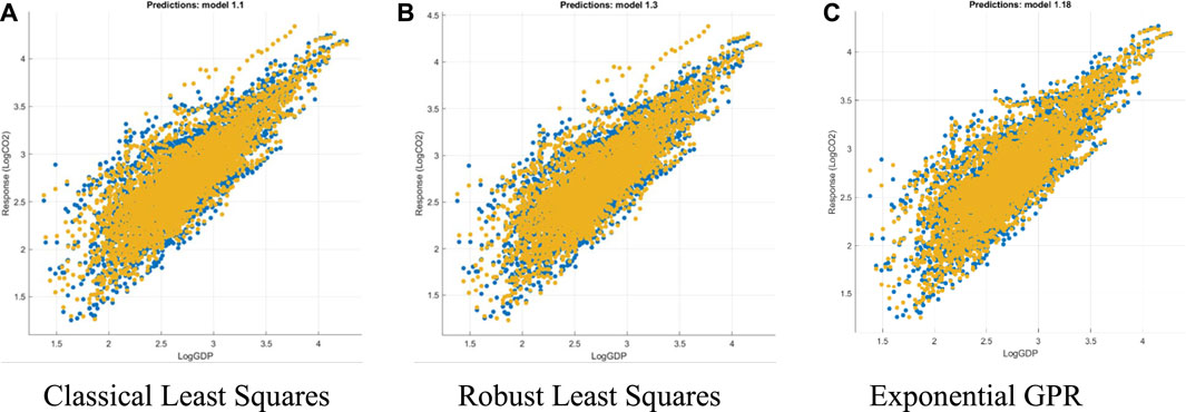
FIGURE 3. Comparing actual and predicted CO₂ emissions against GDP of the selected models. (A) Classical Least Squares. (B) Robust Least Squares. (C) Exponential GPR. Notes: 1) The vertical axis denotes the value of CO2 emissions in the logarithm. 2) The horizontal axis denotes the value of GDP in logarithm. 3) CO₂ emissions are measured in 10,000  tons of standard coal. 4) The blue dots represent actual values whereas the yellow dots represent the predicted values. (5) GDP is measured in 100 million Chinese Yuan.

FIGURE 4

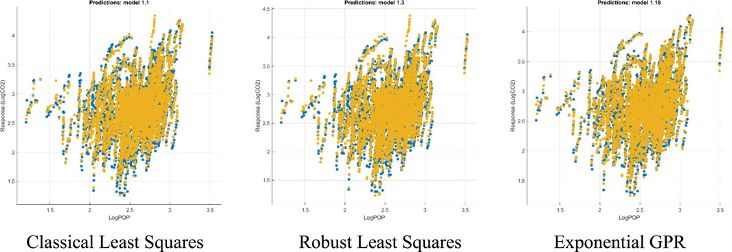
FIGURE 4. Comparing actual and predicted CO₂ emissions against population size of the selected models. Classical Least Squares, Robust Least Squares, Exponential GPR. Notes: 1) The vertical axis represents the value of CO₂ emissions in logarithm. 2) The horizontal axis represents the population size in logarithm. 3) CO₂ emissions are measured in 10,000 tons of standard coal. 4) The blue dots represent actual values whereas the yellow dots represent the predicted values. 5) The unit of population is 10,000 people.

FIGURE 5

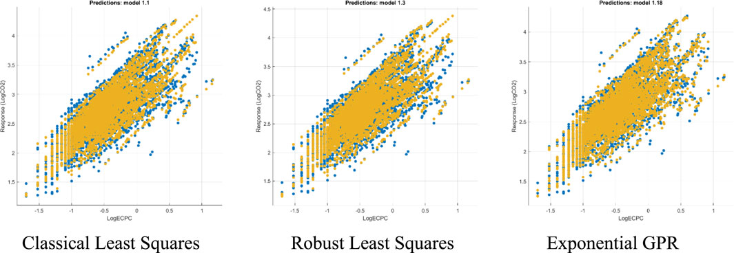
FIGURE 5. Comparing actual and predicted CO₂ emissions against energy consumption of the selected models. Classical Least Squares, Robust Least Squares, Exponential GPR. Notes: 1) The vertical axis represents the value of CO₂ emissions in logarithm. 2) The horizontal axis represents the value of per capita energy consumption in a logarithm. 3) CO₂ emissions are measured in 10,000  tons of standard coal. 4) The blue dots represent actual values whereas the yellow dots represent the predicted values. 5) Per capita energy consumption is measured in tons of standard coal.

FIGURE 6

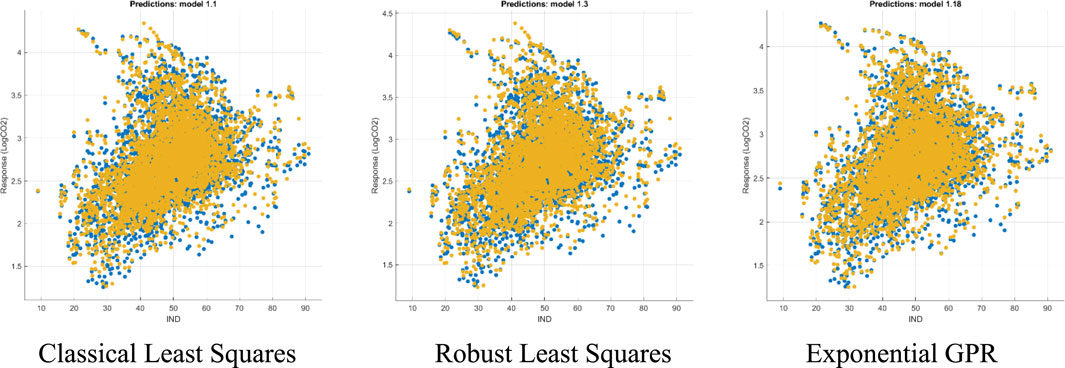
FIGURE 6. Comparing actual and predicted CO₂ emissions against the industrialization of the selected models. Classical Least Squares, Robust Least Squares, Exponential GPR. Notes: 1) The vertical axis represents the value of CO₂ emissions in logarithm. 2) The horizontal axis represents the percentage of secondary industry in China. 3) The blue dots represent actual values whereas the yellow dots represent the predicted values. 4) CO₂ emissions are measured in 10,000 tons of standard coal.

FIGURE 7

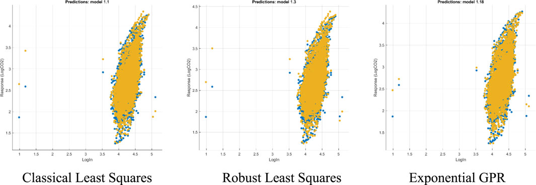
FIGURE 7. Comparing actual and predicted CO₂ emissions against average annual salary of the selected models. Classical Least Squares Robust Least Squares Exponential GPR Notes: 1) The vertical axis represents the value of CO₂ emissions in logarithm. 2) The horizontal axis represents the average annual salary in logarithm. 3) CO₂ emissions are measured in 10,000 tons of standard coal. 4) The blue dots represent actual values whereas the yellow dots represent the predicted values. 5) Average annual salary is measured in the Chinese Yuan.

Figure 3 plots the predicted values of CO₂ emissions against the logarithm of the GDP measured in 10,000 Chinese Yuen. Ideally, it’s convenient if the predicted values are as much closer possible to the actual values for all conducted observations. As shown in Figure 3C predicted CO₂ emissions are quite close to the actual values predicted by using the logarithm of GDP. Even though a small number of deviations can be observed. On the contrary, Figures 3A,B revealed that the classical least squares and the robust least-squares overestimate the CO₂ emissions over the range of 3.2–3.7 logarithm units of GDP. It implies that conditioning on GDP, the Exponential GPR model provides more accurate CO₂ emissions predictions compare with the other two models.

Figures 4–6 show similar results. The predicted CO₂ emissions by using the exponential GPR model are tensed to the actual values over the entire range of population size (see Figure 4), the energy consumption (see Figure 5), and the level of industrialization (see Figure 6). However, when the classical least squares and the robust least-squares model are used, extreme deviations between the actual value and predicted value can be observed. In Figures 4A,B, it is determined that the classical least squares and the robust least-squares model overestimate the CO₂ emissions over the range of 2.7–2.8 logarithm units of population size. Similarly, in Figures 5A,B, CO₂ emissions are overestimated by the classical least squares and the robust least squares models over the range of 0.5–1 logarithm units of per capita energy consumption. In Figure 6, although not obvious, CO₂ emissions are overestimated by the classical least squares and the robust least squares models over the range of 40–50% of secondary industry in China.

Figure 7 shows how the predicted values deviate from the actual values when the independent variable is non-Gaussian for the presence of threshold data points from extreme references. As with the evidence presented above, extreme upward bias over a particular range can be observed when the classical least squares and the robust least squares are used; the models overestimated CO₂ emissions over the range of 4.5– to 4.75 logarithm units of average annual salary. The extreme bias disappears when the exponential GPR model is used. Moreover, when the exponential GPR model is used, the deviations between the actual values and the predicted values are smaller for the extreme data values observed over the range of 1– to 1.5 and 5 to 5.5 logarithm units of average annual salary.

In summary, Figures 3–7 show that predicted CO₂ emissions conditional on individual components (i.e., GDP, population size, energy consumption, and industrialization) are quite close to the actual values predicted using the exponential GPR model. Even the underlying distribution of the independent variable is non-Gaussian. Meanwhile, extreme upward bias per component in the technique can be observed when the classical least squares and the robust least squares models are used. Thus, a conclusion may be drawn upon the study that the exponential GPR model gives the most accurate predictions on CO₂ emissions compared with the remaining models.

Conclusion and Future Works

In this paper, the Gaussian process regression method is proposed for CO₂ emissions analysis in China. The traditional linear regression approach is limited by its rigid functional form and the approach often encounters an over-fitting problem. The Gaussian progress regression approach relaxes the parametric assumption by applying the Bayesian nonparametric inference approach. The preciseness and exactitude of the prediction of the exponential GPR were compared and discussed with the classical least squares and the robust least-squares model. Based on the outcome of the whole study, it is proved that the Gaussian progress regression algorithms can give the most accurate predictions on CO₂ emissions compared with the other two traditional models and thus is applicable for CO₂ emissions prediction analysis to enhance forecast performance.

The prediction performances of the selected methods discussed only focus on the six predominant factors affecting carbon emissions. Future research should focus on further reviewing the completeness of the set of driving factors and the effectiveness of model predictions, compared them with other commonly used models.

Data Availability Statement

The raw data supporting the conclusions of this article will be made available by the authors, without undue reservation.

Author Contributions

NM proposed the conceptualization, methodology and funding acquisition. WS gave the formal data analysis and wrote the original formal draft. TH performed the data collection and original arrangement. FL gave formal methodology, writing-review and editing.

Funding

This study was supported by Hainan College of Economics and Business (Project Reference Number: hnjmk2021301) and the Scientific Research Foundation of Yunnan University of Finance and Economics (No. 2020B03).

Conflict of Interest

The authors declare that the research was conducted in the absence of any commercial or financial relationships that could be construed as a potential conflict of interest.

Publisher’s Note

All claims expressed in this article are solely those of the authors and do not necessarily represent those of their affiliated organizations, or those of the publisher, the editors, and the reviewers. Any product that may be evaluated in this article, or claim that may be made by its manufacturer, is not guaranteed or endorsed by the publisher.

References

Bhattacharya, M., Rafiq, S., Lean, H. H., and Bhattacharya, S. (2017). The Regulated Coal Sector and CO2 Emissions in Indian Growth Process: Empirical Evidence over Half a century and Policy Suggestions. Appl. Energ. 204, 667–678. doi:10.1016/j.apenergy.2017.07.061

CrossRef Full Text | Google Scholar

Birdsall, N. (1992). Another Look at Population and Global Warming. In Policy Research Working Papers ; No. WPS 1020. Population, Health, and Nutrition, 1020. Retrieved from http://documents.worldbank.org/curated/en/985961468766195689/Another-look-at-population-and-global-warming.

Google Scholar

Dinda, S. (2004). Environmental Kuznets Curve Hypothesis: A Survey. Ecol. Econ. 49 (4), 431–455. doi:10.1016/j.ecolecon.2004.02.011

CrossRef Full Text | Google Scholar

Essandoh, O. K., Islam, M., and Kakinaka, M. (2020). Linking International Trade and Foreign Direct Investment to CO2 Emissions: Any Differences between Developed and Developing Countries?. Sci. Total Environ. 712, 136437. doi:10.1016/j.scitotenv.2019.136437

PubMed Abstract | CrossRef Full Text | Google Scholar

Gershman, S. J., and Blei, D. M. (2012). A Tutorial on Bayesian Nonparametric Models. J. Math. Psychol. 56 (1), 1–12. doi:10.1016/j.jmp.2011.08.004

CrossRef Full Text | Google Scholar

Hu, M., Li, R., You, W., Liu, Y., and Lee, C.-C. (2020). Spatiotemporal Evolution of Decoupling and Driving Forces of CO2 Emissions on Economic Growth along the Belt and Road. J. Clean. Prod. 277, 123272. doi:10.1016/j.jclepro.2020.123272

CrossRef Full Text | Google Scholar

Jones, C. I. (1995). R & D-Based Models of Economic Growth. J. Polit. Economy 103 (4), 759–784. doi:10.1086/262002

CrossRef Full Text | Google Scholar

Jorgenson, D. W., and Wilcoxen, P. J. (1993). Reducing U.S. Carbon Dioxide Emissions: an Assessment of Different Instruments. J. Pol. Model. 15 (5-6), 491–520. doi:10.1016/0161-8938(93)90003-9

CrossRef Full Text | Google Scholar

Kahouli, B. (2018). The Causality Link between Energy Electricity Consumption, CO2 Emissions, R&D Stocks and Economic Growth in Mediterranean Countries (MCs). Energy 145, 388–399. doi:10.1016/j.energy.2017.12.136

CrossRef Full Text | Google Scholar

Khan, M., and Rana, A. T. (2021). Institutional Quality and CO2 Emission-Output Relations: The Case of Asian Countries. J. Environ. Manage. 279, 111569. doi:10.1016/j.jenvman.2020.111569

CrossRef Full Text | Google Scholar

Knapp, T., and Mookerjee, R. (1996). Population Growth and Global CO2 Emissions. Energy Policy 24 (1), 31–37. doi:10.1016/0301-4215(95)00130-1

CrossRef Full Text | Google Scholar

Kolstad, C. D., and Krautkraemer, J. A. (1993). “Natural Resource Use and the Environment,”. In Handbook of Natural Resource and Energy Economics. Editors A. V. Kneese, and J. L. Sweeney. 1st ed. Amsterdam North Holland, 3, 1219–1265. doi:10.1016/s1573-4439(05)80013-2

CrossRef Full Text | Google Scholar

Li, R., Wang, Q., Liu, Y., and Jiang, R. (2021). Per-capita Carbon Emissions in 147 Countries: The Effect of Economic, Energy, Social, and Trade Structural Changes. Sustainable Prod. Consumption 27, 1149–1164. doi:10.1016/j.spc.2021.02.031

CrossRef Full Text | Google Scholar

Liu, Y., and Hao, Y. (2018). The Dynamic Links between CO2 Emissions, Energy Consumption and Economic Development in the Countries along "the Belt and Road". Sci. Total Environ. 645, 674–683. doi:10.1016/j.scitotenv.2018.07.062

PubMed Abstract | CrossRef Full Text | Google Scholar

Luo, Y., Zeng, W., Hu, X., Yang, H., and Shao, L. (2021). Coupling the Driving Forces of Urban CO2 Emission in Shanghai with Logarithmic Mean Divisia index Method and Granger Causality Inference. J. Clean. Prod. 298, 126843. doi:10.1016/j.jclepro.2021.126843

CrossRef Full Text | Google Scholar

Mackay, D. J. C. (1998). Introduction to Gaussian Processes. In Neural Networks and Machine Learning. Berlin: Springer.

Google Scholar

Minx, J. C., Baiocchi, G., Peters, G. P., Weber, C. L., Guan, D., and Hubacek, K. (2011). A "Carbonizing Dragon": China's Fast Growing CO2 Emissions Revisited. Environ. Sci. Technol. 45 (21), 9144–9153. doi:10.1021/es201497m

PubMed Abstract | CrossRef Full Text | Google Scholar

Mohmand, Y. T., Mehmood, F., Mughal, K. S., and Aslam, F. (2020). Investigating the Causal Relationship between Transport Infrastructure, Economic Growth and Transport Emissions in Pakistan. Res. Transportation Econ., 100972. doi:10.1016/j.retrec.2020.100972

CrossRef Full Text | Google Scholar

Munir, Q., Lean, H. H., and Smyth, R. (2020). CO2 Emissions, Energy Consumption and Economic Growth in the ASEAN-5 Countries: A Cross-Sectional Dependence Approach. Energ. Econ. 85, 104571. doi:10.1016/j.eneco.2019.104571

CrossRef Full Text | Google Scholar

Nasir, M. A., Canh, N. P., and Lan Le, T. N. (2021). Environmental Degradation & Role of Financialisation, Economic Development, Industrialisation and Trade Liberalisation. J. Environ. Manage. 277, 111471. doi:10.1016/j.jenvman.2020.111471

CrossRef Full Text | Google Scholar

Nguyen, T. T., Pham, T. A. T., and Tram, H. T. X. (2020). Role of Information and Communication Technologies and Innovation in Driving Carbon Emissions and Economic Growth in Selected G-20 Countries. J. Environ. Manage. 261, 110–162. doi:10.1016/j.jenvman.2020.110162

CrossRef Full Text | Google Scholar

Shahbaz, M., Hye, Q. M. A., Tiwari, A. K., and Leitão, N. C. (2013). Economic Growth, Energy Consumption, Financial Development, International Trade and CO2 Emissions in Indonesia. Renew. Sustain. Energ. Rev. 25, 109–121. doi:10.1016/j.rser.2013.04.009

CrossRef Full Text | Google Scholar

Shahbaz, M., Mahalik, M. K., Shah, S. H., and Sato, J. R. (2016). Time-varying Analysis of CO2 Emissions, Energy Consumption, and Economic Growth Nexus: Statistical Experience in Next 11 Countries. Energy Policy 98, 33–48. doi:10.1016/j.enpol.2016.08.011

CrossRef Full Text | Google Scholar

Shi, A. (2003). The Impact of Population Pressure on Global Carbon Dioxide Emissions, 1975-1996: Evidence from Pooled Cross-Country Data. Ecol. Econ. 44 (1), 29–42. doi:10.1016/s0921-8009(02)00223-9

CrossRef Full Text | Google Scholar

Solow, R. M. (1956). A Contribution to the Theory of Economic Growth. Q. J. Econ. 70 (1), 65–94. doi:10.2307/1884513

CrossRef Full Text | Google Scholar

Wang, R., Mirza, N., Vasbieva, D. G., Abbas, Q., and Xiong, D. (2020). The Nexus of Carbon Emissions, Financial Development, Renewable Energy Consumption, and Technological Innovation: What Should Be the Priorities in Light of COP 21 Agreements?. J. Environ. Manage. 271, 111027. doi:10.1016/j.jenvman.2020.111027

CrossRef Full Text | Google Scholar

Williams, C. K. (1998). Learning in Graphical Models. Dordrecht ; Boston: Kluwer Academic Publishers. doi:10.1007/978-94-011-5014-9_23Prediction with Gaussian Processes: From Linear Regression to Linear Prediction and beyond

CrossRef Full Text | Google Scholar

Williams, C. K., and Rasmussen, C. E. (2006). Gaussian Processes for Machine Learning. Cambridge, Mass: Mit Press.

Williams, C. K., and Rasmussen, C. E. (1996). Gaussian Processes for Regression. In Advances in Neural Information Processing Systems. Cambridge, MassLondon: Mit Press.

Google Scholar

Xepapadeas, A. (2005). “Chapter 23 Economic Growth and the Environment,”. Economywide and International Environmental Issues. Editors Karl-GöranM., and J. R. Vincent (Amsterdam: North Holland), 3, 1219–1271. doi:10.1016/s1574-0099(05)03023-8

CrossRef Full Text | Google Scholar

Yuan, J., Xu, Y., and Zhang, X. (2014). Income Growth, Energy Consumption, and Carbon Emissions: The Case of China. Emerging Markets Finance and Trade 50, 169–181.

Google Scholar

Zaidi, S. A. H., Zafar, M. W., Shahbaz, M., and Hou, F. (2019). Dynamic Linkages between Globalization, Financial Development and Carbon Emissions: Evidence from Asia Pacific Economic Cooperation Countries. J. Clean. Prod. 228, 533–543. doi:10.1016/j.jclepro.2019.04.210

CrossRef Full Text | Google Scholar

Zhang, J., Fan, Z., Chen, Y., Gao, J., and Liu, W. (2020). Decomposition and Decoupling Analysis of Carbon Dioxide Emissions from Economic Growth in the Context of China and the ASEAN Countries. Sci. Total Environ. 714, 136649. doi:10.1016/j.scitotenv.2020.136649

PubMed Abstract | CrossRef Full Text | Google Scholar

Zhang, Y.-J., Liu, Z., Zhang, H., and Tan, T.-D. (2014). The Impact of Economic Growth, Industrial Structure and Urbanization on Carbon Emission Intensity in China. Nat. Hazards 73 (2), 579–595. doi:10.1007/s11069-014-1091-x

CrossRef Full Text | Google Scholar