Improved Random Forest Method for Ultra-short-term Prediction of the Output Power of a Photovoltaic Cluster

Current models for the prediction of the output power of photovoltaic (PV) clusters suffer from low prediction accuracy and are prone to overfitting. To address these problems, we propose an improved random forest (RF)-based method for ultra-short-term prediction of PV cluster output power. The total output power data for the PV clusters are used as the training dataset and fed into the RF model to obtain preliminary predictions. The error and accuracy of the preliminary predictions for individual sampling points concerning the actual values of the PV cluster output power are assessed. Each of the daily time series of preliminary predictions is divided into two phases according to whether the output power is increasing (morning) or decreasing (afternoon). The final ultra-short-term predictions of the PV cluster output power are obtained by correcting the two phases of preliminary predictions through trend correction and peak correction, respectively. The results show that, compared with the unimproved model, the accuracy of the stochastic forest model is 1.48% higher than that of the modified random forest model., which proves the effectiveness and practicability of the proposed method.

Introduction

Traditional fossil fuels, including coal, petroleum, and natural gas (Chen, 2019), currently account for the majority of global energy consumption. However, their use produces large amounts of greenhouse gases, other harmful gases, and waste, all of which threaten environments all over the world. New energy sources are attracting increasing attention. In particular, solar energy is increasingly widely used, due to its advantages of zero emissions, zero pollution, and no limitations in geographical resource allocation; this has led to photovoltaic (PV) generation technology becoming an important research topic (Jing et al., 2017). PV clusters that integrate multiple PV stations are an increasingly popular model of PV generation. However, due to the inherent properties of the output power of PV clusters, ensuring the balance and stability of the grid necessitates the effective planning and scheduling of the electric energy that is input and output (Pang, 2017). Operating costs must also be considered in the assessment of the expense of a normal power supply (Li et al., 2020). The effective prediction of PV output power is among the most important steps in the study of grid.

PV output power predictions can be classified as ultra-short-term (0–4 h), short-term (0–72 h) and medium-to-long-term (1 month–1 year) predictions according to their time scale (Yang et al., 2018a). Methods of predicting PV output power can be grouped into numerical weather prediction (NWP) (Xu et al., 2016), an environmental factor-based physical method, and a historical data-based statistical method and learning method. A previous study (Savarimuthu and Victor, 2020) explains the relationship between the bonding between current, power, and the potential developed in the solar PV module and the consequences of changes in solar insolation levels on the parameters involved. A PV output power periodicity extraction and locality sensitive hashing (LSH)-based ultra-short-term prediction method has been proposed (Yang and Huang, 2018). The periodicity of PV output power includes extraction of the periodic components. For the remaining components, the LSH algorithm is used to achieve the rapid classification of PV power segments under different weather conditions, and Euclidean distance is adopted as a classification measure. This method was verified using data from PV stations, demonstrating high prediction accuracy. A previous study (Yang et al., 2018b) classified weather conditions into four types according to the weather forecast—namely, sunny, cloudy, overcast, and rainy—and proposed an adaptive network-based fuzzy inference system (ANFIS) model for ultra-short-term prediction of PV output power in different types of weather conditions. The initial structure of the fuzzy inference system was created using a subtractive clustering algorithm, thereby effectively avoiding the problem of combinatorial explosion. The proposed model had good prediction accuracy for all weather conditions, confirming the effectiveness of the proposed method. Another method of predicting PV output power has been proposed that uses the gradient boosting decision tree (BOA-GBDT), a fine-grained, feature-based Bayesian optimization algorithm (Chen et al., 2018). This method first created instantaneous weather model features and time window trend features and then reasonably reduced the number of types of fine-grained features using the BOA. It ultimately fitted the relationship between the features and the PV output power curve using the GBDT model, thereby greatly reducing its running time and error. A deep random forest (RF) algorithm in two stages, namely, multi-grained scanning and cascade forest stages has been found not to require human adjustment of the parameters, as is required for deep neural networks (Cui et al., 2020). A machine learning-based technique has been shown to be capable of predicting the short-term output power of PV–wind hybrid power generation clusters (Yan et al., 2014). This technique first identifies typical power stations in individual regions based on the correlation between the historical output power data of individual power stations in individual regions and the total output power data of individual regions to predict the total output power of the cluster using a weighted-error, back propagation neural network (BPNN). The overall performance of the proposed technique is slightly better than that of the build-up method; however, as the number of stations in the cluster increases, the prediction error of the proposed technique becomes slightly higher than that of the build-up method.

To address the problem of the low predictability of the PV output power using traditional RF ultra-short-term prediction, we propose a method for ultra-short-term prediction of PV cluster outputs that corrects noontime prediction accuracy loss through peak correction. The method first performs preliminary predictions for individual sampling points using an RF model and then divides each of the daily time series of preliminary predictions into morning and afternoon phases. For the morning phase, the phase relationship between the preliminary predictions and the actual values was adjusted using a discrete grey prediction model (DGM), thereby obtaining corrected ultra-short-term predictions. The experimental results show that the improved model outperforms the original in terms of fitting capacity, prediction error, and accuracy.

RF Model

The RF regression algorithm is an important application of RF theory, a statistical learning method proposed by Breiman in 2001 (Xu, 2013). It takes multiple samples from the source using a bootstrap resampling method, establishes a decision-tree model for each bootstrap sample set, combines the decision trees for prediction, and averages the predictions to obtain a final prediction. In essence, the algorithm uses decision trees as base learners and assembles them to create a forest. The algorithm has a high prediction accuracy and controllable generalization error, is capable of rapid convergence, requires the adjustment of fewer parameters, and can effectively avoid overfitting; thus, it is suitable for the computation of a variety of datasets, such as ultra-high-dimensional characteristic vector spaces (Breiman, 1996). Its core idea is to combine several weakly performing classification and regression trees (CARTs) into a forest according to certain rules to obtain final results based on the voting of all of the decision trees in the forest.

RF regression increases the difference between the classification models by creating different training datasets, thereby increasing the capacity of the combined classification models for extrapolative prediction. Through k rounds of training, a series of classification models $\left\{h_1\left(X\right), h_2\left(X\right), \dots ,h_k\left(X\right)\right\}$ is obtained, which is then used to create a system of multiple classification models. The final classification decision can be expressed as:

$H\left(x\right)=\arg \underset{Y}{max}{\displaystyle \sum _{i=1}^{k}I\left(h_i\left(x\right)=Y\right)}(1)$

where H(X) is the combined classification model, h_i is the ith individual decision-tree classification model, Y is the output variable (or target variable), and I (·) is a characteristic function. Eq. 1 denotes the final classification using a simple majority voting method.

For each of a given set of classification models $\left\{h_1\left(X\right), h_2\left(X\right), \dots ,h_k\left(X\right)\right\}$, the training dataset was taken from the source dataset (X, Y) through random sampling; thus, the margin function can be expressed as:

$mg\left(X,Y\right)=a{v}_{k}I\left(h_k\left(X\right)=Y\right)-maxa{v}_{k}I\left(h_k\left(X\right)=j\right)(2)$

The margin function measures the degree to which the average number of correct classifications exceeds the average number of incorrect classifications. A larger margin indicates higher reliability of classification prediction. The extrapolative error (or generalization error) can be expressed as:

$P{E}^{\ast }=P_{X,Y}\left(mg\left(X,Y\right)<0\right)(3)$

As can be proven, as the number of decision-tree classification models increases, all series Θ₁ …PE* converge almost everywhere on:

$P_{X,Y}\left(P_{\Theta }\left(h\left(X,\Theta \right)=Y\right)\right)-\underset{j\ne Y}{\max }{P}_{\Theta }\left(h\left(X,\Theta \right)=j\right)<0(4)$

Therefore, the RF regression method does not have the problem of overfitting as the number of decision trees increases.

CART is a binary recursive partitioning technique (Zhang, 1997), with the current sample set split into two subsets at each of the nodes (except for leaf nodes). The CART algorithm uses the Gini Index as the attribute selection criterion. If we suppose that dataset D contains m classes, the Gini Index G_D can be obtained with the following equation:

$G_D=1-{\displaystyle \sum _{j=1}^m{p}_j^2}(5)$

where p_j is the frequency of occurrence of the jth class of elements.

The Gini Index needs to consider the binary partition on each attribute (Huang et al., 2019a). Suppose dataset D is split into D1 and D2 through a binary partition on attribute A; then the Gini Index for splitting sample set D on attribute A at this subnode can be expressed as:

$G_{D,A}=\frac{\left|D_1\right|}{D}{G}_{D1}{D}_1+\frac{\left|D_2\right|}{D}{G}_{D2}{D}_2(6)$

For each attribute, all possible binary partitions are considered, and the partition with the lowest Gini Index is used. Therefore, a smaller Gini Index for attribute A G_{D, A} indicates a better partition for attribute A. Following this rule, splitting is performed in a recursive, top-down manner until a complete decision tree is created (Zhang, 1997; Zhu, 2006).

RFs have the following statistical advantages:

1) They only need to adjust two parameters, namely, the number of trees in the forest N_tree and the number of features selected for splitting each tree M_try.

2) As guaranteed by the law of large numbers, RFs have a very high classification accuracy and are not prone to overfitting.

3) Another characteristic of RFs is their out-of-bag (OOB) estimate. When training subsets are generated through bagging, close to 37% of the samples in the source set do not fall into the training subset for any CART. These samples are referred to as OOB samples, and they can be used to estimate the generalization error of the RFs and to compute the importance of individual features (Huang et al., 2018; Huang et al., 2019b).

The simplest random feature selection for RFs is the random selection of a small number F of input variables for splitting at each node. In this way, the splitting of the decision tree at each node can be based on the selected F features, so not all of the features need to be examined. Then, complete trees are grown using the CART method that does not need pruning, thus facilitating the minimization of the skewness of the trees. Once the decision trees are grown, ensemble predictions can be performed using the majority voting method. This process is a random selection of input variables. F input variables, a fixed number, are selected to establish an RF. To increase randomness, bootstrap samples of the input variables can be generated using the bagging method. Both the strength and correlation of RFs depend on the value of F. The correlation between the trees decreases with F, and the strength of classification models increases with F. After being verified, only one subset of an input variable needs to be considered at each node, thereby significantly reducing the running time of the algorithm.

Figure 1 shows the decision-making process of the RF models.

FIGURE 1

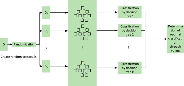
FIGURE 1. Working principles of the random forest model.

Establishment of an Improved RF-Based Ultra-short-term PV Cluster Output Power Prediction Model

Preliminary Predictions

There are three main strategies for predicting the output power of PV clusters consisting of distributed stations, namely, build-up, spatial upscaling, and ensemble strategies. The build-up strategy obtains predictions for individual stations and stacks the final predictions for those stations to obtain the overall final prediction for the output power of the entire cluster. The spatial upscaling strategy divides a cluster into several regions following certain rules and stacks the weighted predictions for stations that best represent the output power of the respective regions to obtain the predictions for the entire cluster. The ensemble method, which is the simplest and most straightforward one, obtains predictions for the total output power of the entire cluster using the historical total output power data of the cluster as training data (Yang et al., 2020).

There are no state variables that cover a large area, such as historical weather conditions or NWP, for the entire cluster; there are only temporal features, such as different sunrise and sunset times and maximum irradiance times (or peak output-power times) at the geographical location of the PV cluster in different seasons. Therefore, the set-pair method and RF model were used, because neither method requires a state variable. Using data from the previous 30 days as the training data, the output power of a PV cluster in Northeast China over 5 days (numbered days 76–80) in 2019 was predicted using build-up and ensemble strategies separately, and the prediction errors were comparatively analyzed. The cluster consisted of 20 stations, had a total output power of 650 MW, and was sampled every 15 min. Table 1 shows the results.

TABLE 1

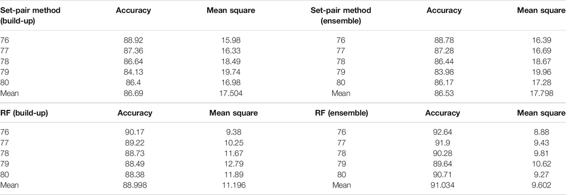
TABLE 1. Comparison of prediction methods and strategies.

Due to the influence of the pooling effect in the output power of the cluster, the predictions yielded by the ensemble strategy using the RF model for the 5 days had smaller prediction errors compared to those yielded by the build-up strategy. The RF model improved the accuracy of the predictions for the 5 days by 2.47, 2.68, 1.55, 1.15, and 2.33%, respectively, and by 2.03% on average. The set-pair method had lower accuracy, with an average accuracy for the 5 days that was 1.6% lower. Therefore, the RF model and the ensemble strategy were used for predicting the output power of the PV cluster.

Correction of Preliminary Predictions

To address the problem of the loss of prediction accuracy for the RF model, the preliminary predictions were corrected using the peak correction method. The daily time series of output power data was divided into morning and afternoon phases:

Morning (or increasing) phase: because the sampling points are before the peak output power time, the correction was made using the peak output power predicted based on the trend.

Afternoon (or decreasing) phase: because the time of maximum output power has already occurred, the correction was made using the current maximum output power.

If P_tmax > P_max, the:

$P_i^{\prime }= \left(1-\left|\frac{P_{tmax}-P_{imax}}{P_{tmax}}\right|\right)P_i(7)$

If P_tmax < P_max, then:

$P_i^{\prime }= \left(1+\left|\frac{P_{tmax}-P_{imax}}{P_{imax}}\right|\right)P_i(8)$

where P_i is the preliminary prediction for the ith sampling point, P_imax is the maximum of the preliminary predictions, P_i^′ is the correction, and P_tmax is the maximum of the observations up to the current sampling point.

The output power predictions for the morning phase were corrected using a different method because different from that of the afternoon phase, as the PV output power in the morning phase gradually increases with solar irradiance, and the actual peak output power of the prediction day is unknown at the time of prediction (Li and Fang, 2009).

The DGM(1,1) has a broader modeling mechanism than GM(1,1) and can effectively avoid the error between the whitening model and the whitening equation (Lin et al., 2013; Jiang et al., 2014; Yang et al., 2021). In this study, the increasing trend for PV output power was predicted using the metabolic DGM(1,1) model, which replaces the oldest information x₍₀₎(1) with the latest information x₍₀₎(k+1) to predict the following set of data. The grey model varies with time. For the DGM(1,1) model, suppose there is a source series as follows:

$X^{\left(0\right)}=\left(x^{\left(0\right)}\left(1\right),x^{\left(0\right)}\left(2\right),\dots ,x^{\left(0\right)}\left(n\right)\right)(9)$

then the following equation is referred to as DGM(1,1) model:

$x^{\left(1\right)}\left(k+1\right)=\gamma x^{\left(1\right)}\left(k\right)+\rho (10)$

Designate the first-order accumulating generation operator as α⁽¹⁾:

${\alpha }^{\left(1\right)}{x}^{\left(1\right)}=x^{\left(1\right)}\left(k\right)-x^{\left(1\right)}\left(k-1\right),k=2,\dots ,n(11)$

$x^{\left(1\right)}\left(k\right)={\displaystyle \sum }_{i=1}^k{x}^{\left(0\right)}\left(i\right),k=\mathrm{1,2},\dots ,n(12)$

then the following equation is referred to as the whitening equation of the DGM(1,1) model:

$\frac{d^2}{d{t}^2}+\gamma \frac{d{x}^{\left(1\right)}}{dt}=\rho (13)$

Suppose:

$B=\left[\begin{array}{cc}-x^{\left(1\right)}\left(1\right)& 1\\ -x^{\left(1\right)}\left(2\right)& 1\\ ⋮& ⋮\\ -x^{\left(1\right)}\left(n-1\right)& 1\end{array}\right],\text{Y}=\left[\begin{array}{c}{x}^{\left(1\right)}\left(2\right)\\ x^{\left(1\right)}\left(3\right)\\ ⋮\\ x^{\left(1\right)}\left(n\right)\end{array}\right](14)$

then the least-square estimate of the parameter $\widehat{\alpha }={\left[\gamma \rho \right]}^T$ of DGM(1,1) is:

$\widehat{\alpha }={\left(B^{T}B\right)}^{–1}{B}^{T}Y(15)$

Finally, the mathematical model of the source series can be expressed as:

$x^{\left(0\right)}={\alpha }^{\left(1\right)}{x}^{\left(1\right)}\left(k\right)=\left(\gamma -1\right)\left[x^{\left(0\right)}\left(1\right)-\frac{\rho }{1-\gamma }\right]{\gamma }^{k-1}(16)$

For example, the time series of the output power of the cluster, beginning from the time of startup, is predicted at moment t = 4 using DGM(1,1), as follows: The time series was reversed and then fed into the DGM(1,1) model for prediction, yielding (t₂, Y_t2), which has an angle of φ with respect to the x-axis. Another straight line runs through the starting point of prediction t₅ and the point of the maximum of predictions t₁₁. The two straight lines are translated such that they converge at (t₄, Y_t4). Accuracy is maximized when the two straight lines have the same slope.

The preliminary predictions yielded by the RF model for the morning phase can be corrected using the following equation:

$P{\mathrm{\prime }}_i=\left(P_i-P_x\right)\times \frac{\tan \phi }{\tan \theta } \left(i=\mathrm{1,2},\dots ,16\right)(17)$

$\tan \phi =\frac{Y_{t-1}-Y_{t-3}}{2}, \tan \theta =\frac{P_{imax}-P_1}{t_{P_{max}}-t_1}(18)$

where P_i is the preliminary prediction for the ith sampling point, P_i^′ is the correction, P_x is the actual output power at the current moment, Y_t is the observed output power, and $t_{P_{max}}$ is the moment of the peak output power predicted based on the trend.

Prediction Process of Improved RF-Based Ultra-short-term PV Cluster Output Power Prediction Model

Figure 2 shows the prediction process.

FIGURE 2

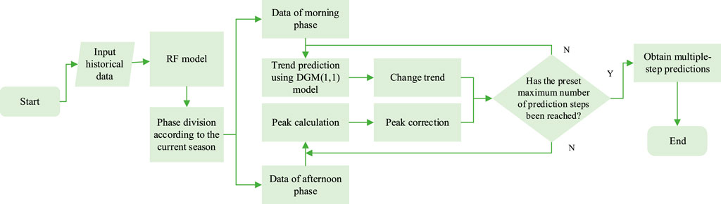
FIGURE 2. Improved stochastic forest model process.

Selection of Assessment Indexes

The model was assessed using the root mean square error (RMSE) and accuracy. These two indexes were calculated using the following equations:

$RMSE= \sqrt{\frac{1}{n}{\displaystyle \sum }_{i=1}^n{\left[\frac{\tilde{P}\left(i\right)-P\left(i\right)}{P_{cap}}\right]}^2}\times 100\%(19)$

where $\tilde{P}\left(i\right)$ is the predicted PV output power, P(i) is the actual PV output power, $P_{cap}$is the total installed capacity of the station, n is the length of the sampling point, and i is the serial number of the sampling point of prediction.

Average prediction accuracy:

$r_{1i}=\left[1-\sqrt{\frac{1}{n}{\displaystyle \sum }_{i=1}^n{\left(\frac{\tilde{P}\left(i\right)-P\left(I\right)}{P_{cap}}\right)}^2}\right]\times 100\%(20)$

$r_1=\frac{1}{n}{\displaystyle \sum }_{i=1}^n{r}_{1i}(21)$

where r_1i is the prediction accuracy at the ith point, and r₁ is the average prediction accuracy.

Testing and Analyses

Analyses of Preliminary Predictions

The output power of a PV cluster in Jilin Province, China over 7 consecutive days in March 2019 was predicted using 90 and 10% of the total output power data of 5,760 clusters in the 60 days prior to the prediction days as the training and testing datasets, respectively. Table 2 presents the results.

TABLE 2

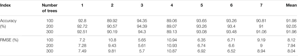
TABLE 2. Forecast results using 60-days historical data.

For a given period of historical data, prediction runs using different numbers of trees yielded largely similar results. Thus, the number of trees has a nonsignificant effect on the classification process and results. However, this may be due to an inadequate amount of time series data; thus, further verification was performed by increasing the length time considered.

Further prediction runs were performed using 90 and 10% of the total output power data of 2,880 clusters over the 30 days prior to the prediction days as the training and testing datasets, respectively. Table 3 shows the results.

TABLE 3

TABLE 3. Forecast results using 30-days historical data.

The prediction runs using different numbers of trees yielded markedly different results depending on the length of the period considered. A shorter span of time series data improved the quality of the predictions. Following the preliminary predictions, the parameters of the RF model were configured as follows: using the data of 2,880 clusters in 30 days prior to the prediction day as the training data; N_tree = 100.

Using the data of the cluster from January to June 2019 as the training dataset for the preliminary prediction, the ultra-short-term prediction was performed using the RF model. Figure 3 shows the monthly RMSE error frequency curves. Table 4 shows the monthly average prediction accuracies and RMSEs.

FIGURE 3

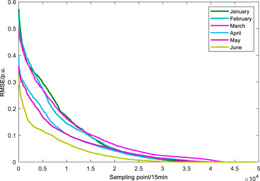
FIGURE 3. Monthly root mean square error frequency curve.

TABLE 4

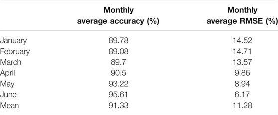
TABLE 4. Monthly average indexes of preliminary predictions.

Figure 4 shows the daily accuracy curves of the ultra-short-term predictions yielded by the RF model for 180 days (January to June) in 2019. As shown in Figure 5, the predictions yielded by the RF model for noon (high output power) have large errors, and the prediction accuracy of the 35th to 55th sampling points were generally lower than 80%, greatly affecting the overall prediction accuracy of the model.

FIGURE 4

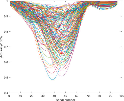
FIGURE 4. Daily forecast accuracy curve for each day from January to June in 2019.

FIGURE 5

FIGURE 5. Daily forecast accuracy from April to June.

As shown in Figure 5, the predictions for April to June had relatively high accuracies, namely, 90.50, 93.22, and 95.61%, respectively; however, the model failed to identify the peak output power.

Figure 7 shows the daily curves of the observed cluster of actual total output power in June 21–30. The daily average prediction accuracies for June 24 and 30 were 94.6 and 95.72%, respectively. As shown in Figures 6–10, the correlations of prediction accuracy and error of the RF model with the level of PV cluster output power are nonsignificant, with the prediction accuracy remaining above 93% for sampling points with the lowest level of output power. The weather type of the entire cluster cannot be defined due to the geographically scattered distribution of the stations. As noted earlier, low-accuracy sampling points mainly occur in the range of the 35th to 55th sampling points, i.e., the period corresponding to the peak output power. Therefore, the accuracy loss in prediction for noon was corrected through peak correction.

FIGURE 6

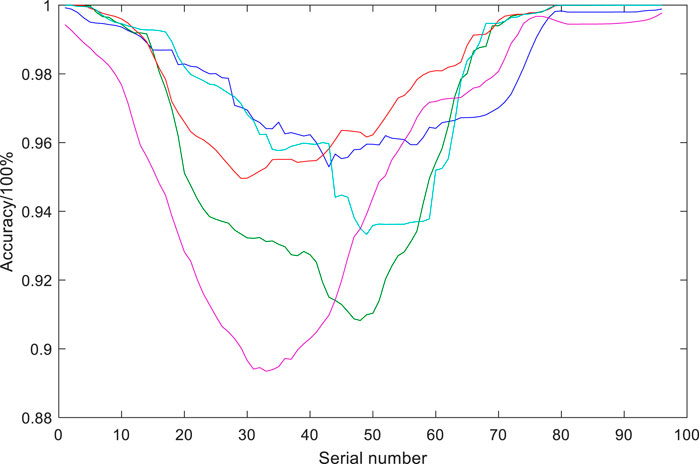
FIGURE 6. Daily prediction accuracy curves for the 5 days with the highest daily average prediction accuracy.

FIGURE 7

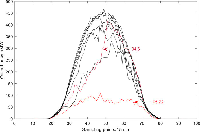
FIGURE 7. Daily curves for observed cluster total output power from 21 to 30 June.

FIGURE 8

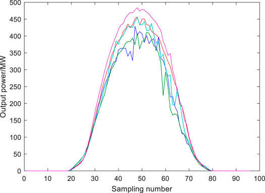
FIGURE 8. Daily observed output power curves for the 5 days with the highest prediction accuracy.

FIGURE 9

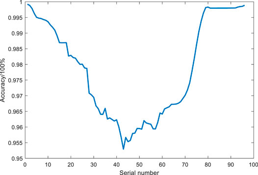
FIGURE 9. Prediction accuracy at individually sampled points for June 21, the day with the highest daily average prediction accuracy.

FIGURE 10

FIGURE 10. Sampling points with the highest prediction accuracy for June 21, the day with the highest daily average prediction accuracy.

Because the sunrise and sunset times in the geographical location of the cluster are different or because the time of peak output power is different in different seasons it is necessary to identify the critical point of the daily increasing and decreasing trends of the total output power of the cluster in different seasons. For example, the seasonal critical points of a PV cluster in Jilin Province were identified using the daily observational data of the cluster’s 20 stations in 2028 at a sampling interval of 15 min. First, the daily time points of peak output power were identified, as shown in Figure 2.

The time point of maximum output power in the cluster occurred at the 49th sampling point in 25 days from January to March (a ), at the 47th sampling point in 18 days from April to June (b ), at the 47th sampling point in 14 days from July to September (c ), and at the 47th sampling point in 14 days from October to December (d ) (Figure 11). The seasonal time points of maximum output power identified above were used to identify the respective seasonal critical points between the daily increasing and decreasing trends of cluster output power, thereby minimizing prediction error.

FIGURE 11

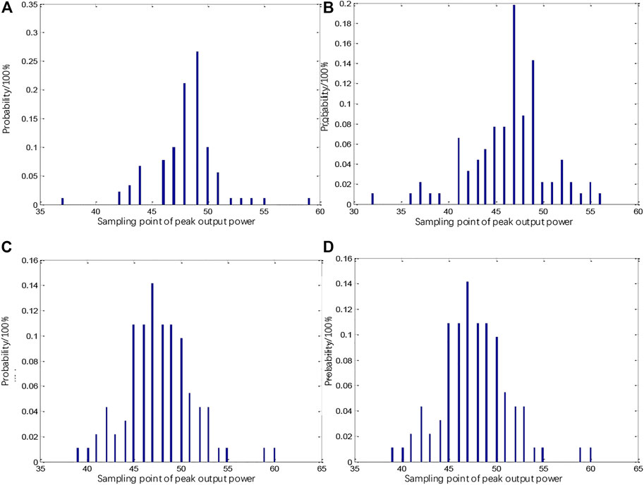
FIGURE 11. Sampling points with daily peak cluster output power in different seasons.

Correction of Preliminary Predictions

As shown in Figures 12,13 the preliminary predictions for January 21 (observed peak output power was 391.16 MW) showed a peak output power of 218.36 MW, daily average prediction accuracy of 88.38%, and an RMSE of 16.10%, while the improved predictions showed a peak output power of 390.9 MW, daily average prediction accuracy of 89.09%, and an RMSE of 14.54%. After correcting the predictions for all sampling points in the afternoon phase separately, the monthly average prediction accuracy for January 2019 improved from 89.89 to 91.76%, and the RMSE decreased from 14.42 to 11.21%.

FIGURE 12

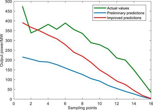
FIGURE 12. Comparison of results before and after improvement in the afternoon phase.

FIGURE 13

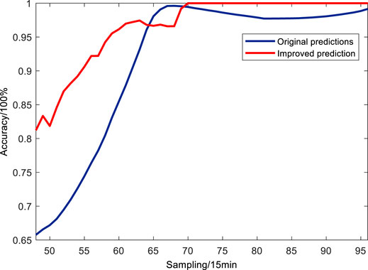
FIGURE 13. Prediction accuracy of each step after improved prediction in the afternoon phase.

As shown in Figures 14,15, the output power predictions for the morning phase were corrected using a different method because, unlike the afternoon phase, PV output power in the morning phase gradually increases with solar irradiance, the actual peak output power of the prediction day is unknown at the time of prediction, and the actual peak is not available for correcting the preliminary predictions yielded by the RF model. For example, the daily average prediction accuracy and RMSE for January 21 before the correction of the morning phase were 90.76 and 13.26%, respectively, while after the correction they were 93.16 and 10.44%, respectively. The monthly average accuracy improved from 97.16 to 92.55%, and the monthly average RMSE decreased from 11.21 to 9.87%.

FIGURE 14

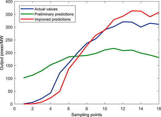
FIGURE 14. Comparison of results before and after improvement in the morning phase.

FIGURE 15

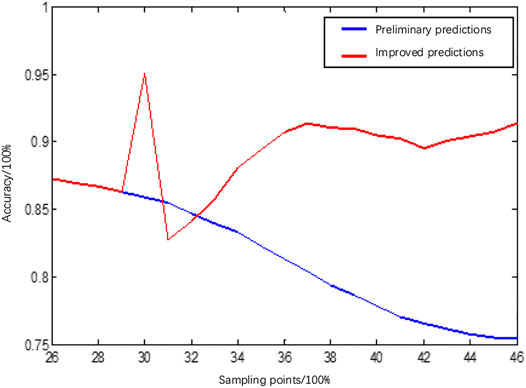
FIGURE 15. Prediction accuracy at individual sampling points in the morning phase after improvement.

From Figures 16,17, it can be seen that the PV power curve has an obvious upward trend in the morning period. Both the Persistence method and the RF method have poor effects and cannot track the actual power well. The Rank-set pair method is compared the prediction effect of the first two methods is better, but the prediction effect of the time period before the 8th sample point is still not ideal, and the Improved RF prediction model proposed in this paper has the best effect, which fits the full curve of actual photovoltaic output best; in the afternoon, it can be seen that the photovoltaic power curve has a clear downward trend and fluctuates to varying degrees. The Improved RF method proposed in this paper has a significant correction before the improvement, so that the predicted curve is closer to the actual photovoltaic output curve. At the same time, combined with the morning from the graph in the afternoon, the peak correction method has significantly improved the accuracy of the prediction model.

FIGURE 16

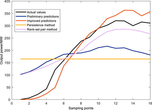
FIGURE 16. Comparison of predictions for the morning phase yielded by different methods.

FIGURE 17

FIGURE 17. Comparison of predictions for the afternoon phase yielded by different methods.

Comparison With Other Methods

As shown in Table 5, compared to persistence and rank-set pair methods, the improved RF ultra-short-term prediction model proposed above improved the monthly average prediction accuracy by 5.64 and 1.77% and reduced the RMSE by 7.95 and 5.09%, respectively, outperforming the other two prediction models in terms of all assessment indexes. Compared to the original version, the improved version of the RF model improved prediction accuracy by 1.48% and reduced RMSE by 2.94%. The daily maximum RMSE is not larger than 15%. After correction for both the morning and afternoon phases, the prediction accuracy improved by 5.23%, and the RMSE decreased by 4.65%. The results show that the correction method proposed in this paper can effectively improve the ultra-short-term prediction accuracy of photovoltaic cluster power, and has certain credibility and wide applicability.

TABLE 5

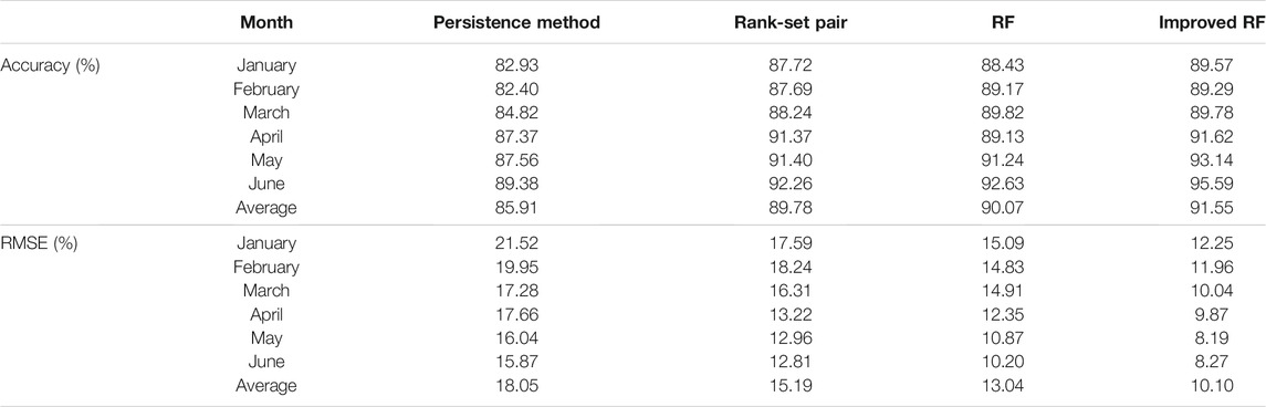
TABLE 5. Comparison of results for each prediction method.

Conclusion

To further improve the accuracy of output power prediction of PV, we proposed an RF model for ultra-short-term prediction of PV cluster output power that considers the characteristics of particular PV clusters and makes corrections based on them. The model was through application to observational datasets. The results are summarized as follows:

1) The model was tested using time series of historical data of different lengths and with different parametric settings. For a given period of data, changing the number of trees in the model does not affect the model’s performance. For a given number of trees, decreasing the span of data greatly improves the prediction accuracy of the model. Based on these findings, the model was preliminarily optimized for subsequent predictions.

2) The predictions yielded by the RF model with optimized parameters were analyzed. The results show that the traditional RF model fails to identify the peak output power for various levels of the actual output power. Considering that a PV cluster usually consists of stations distributed over a large geographical region, and it is difficult to define the state characteristics of the entire cluster, the error of output power predictions is corrected through peak correction.

3) In contrast to BPNN and other artificial intelligence methods, the improved RF based ultra-short-term PV cluster output power prediction method corrects the trends in the morning and afternoon phases and the peak output power, thus better reflecting the trend characteristics of the output power and having a stronger fitting power. Relative to the original version, the improved version of the RF model reduces error by 4.65% and improves prediction accuracy by 5.23%.

Data Availability Statement

The data analyzed in this study is subject to the following licenses/restrictions: Requests to access these datasets should be directed to MZ, 18686624544@163.com.

Author Contributions

MY is responsible for the work concept or design MZ is responsible for data collection DL is responsible for drafting the paper MM made important revisions to the paper The final version of the paper approved by XS for publication.

Conflict of Interest

Author DL is employed by Changchun Power Supply Branch of Jilin Electric Power Co., Ltd. of STATE GRID Corporation of China.

The remaining authors declare that the research was conducted in the absence of any commercial or financial relationships that could be construed as a potential conflict of interest.

Publisher’s Note

All claims expressed in this article are solely those of the authors and do not necessarily represent those of their affiliated organizations, or those of the publisher, the editors and the reviewers. Any product that may be evaluated in this article, or claim that may be made by its manufacturer, is not guaranteed or endorsed by the publisher.

Acknowledgments

This work was supported by the National Key R&D Program of China (Technology and application of wind power/photovoltaic power prediction for promoting renewable energy consumption, 2018YFB0904200).

References

Breiman, L. (1996). Bagging Predictors[J]. Machine Learn. 24 (2), 123–140. doi:10.1007/bf00058655

CrossRef Full Text | Google Scholar

Chen, L., Yin, L., and Tao, Y. (2018). Short-term Power Load Prediction Based on Deep forest Algorithm [J]. Electric Power Construction. 39 (11), 42–50.

Google Scholar

Chen, X. (2019). Photovoltaic Energy Will Phase Out Fossil Energy in Ten Years [J]. Energ. Conservation Environ. Prot. (1), 27–29.

Google Scholar

Cui, Y., Chen, Z., and Xu, P. (2020). Short-Term Power Prediction for Wind Farm and Solar Plant Clusters Based on Machine Learning Method [J]. Electric Power. 53 (3), 1–7.

Google Scholar

Huang, N., Wang, D., Lin, L., Cai, G., Huang, G., Du, J., et al. (2019a). Power Quality Disturbances Classification Using Rotation Forest and Multi‐Resolution Fast S‐Transform With Data Compression in Time Domain, IET Generation, Transm. Distribution. 13, 5091–5101. doi:10.1049/iet-gtd.2018.5439

CrossRef Full Text | Google Scholar

Huang, N., Wu, Y., Cai, G., Zhu, H., Yu, C., Jiang, L., et al. (2019b). Short-Term Wind Speed Forecast With Low Loss of Information Based on Feature Generation of OSVD. IEEE Access. 7, 81027–81046. doi:10.1109/access.2019.2922662

CrossRef Full Text | Google Scholar

Huang, N., Xing, E., Cai, G., Yu, Z., Qi, B., and Lin, L. (2018). Short-Term Wind Speed Forecasting Based on Low Redundancy Feature Selection. Energies. 11 (7), 1638. doi:10.3390/en11071638

CrossRef Full Text | Google Scholar

Jiang, X., Chen, H., and Hu, X. (2014). Research of Prediction Error Uncertainty-Based Large-Scale Integration of Intermittent Power Generation Units. Power Syst. Tech. 38 (9), 2455–2460.

Google Scholar

Jing, B., Tan, L., and Zheng, Q. (2017). An Overview of Research Progress of Short-Term Photovoltaic Forecasts [J]. Electr. Meas. Instrumentation. 54 (12), 1–6.

Google Scholar

Li, B., and Fang, L. (2009). Conditions for Function Transformation to Improve the Accuracy of Grey Prediction Model. J. Logistical Eng. Univ. 25 (4), 86–90.

Google Scholar

Li, C., Zhou, H., Li, J., and Dong, Z. (2020). Economic Dispatching Strategy of Distributed Energy Storage for Deferring Substation Expansion in the Distribution Network With Distributed Generation and Electric Vehicle. J. Clean. Prod. 253, 119862. doi:10.1016/j.jclepro.2019.119862

CrossRef Full Text | Google Scholar

Lin, S., Han, M., and Zhao, G. (2013). Capacity Allocation of Energy Storage in Distributed Photovoltaic Power System Based on Stochastic Prediction Error [J]. Proc. CSEE. 33 (4), 25–33+5.

Google Scholar

Pang, M., Zhou, D., Chen, Y., Zhong, K., Xin, Y., Qin, R., et al. (2017). Analysis of Spatial and Temporal Distribution of Downward Surface Shortwave in Xinjiang Based on CERES Data [J]. Desert Oasis Meteorol.

Google Scholar

Savarimuthu, L. J., and Victor, K. (2020). Photo Voltaic (PV) Cell Characteristics Design Using M.File in Matlab [J]. Int. J. Innovative Tech. Exploring Eng. 9 (3), 2278–3075. doi:10.35940/ijitee.c7990.019320

CrossRef Full Text | Google Scholar

Xu, B. (2013). Research of Random Forest Algorithm Optimization for High-Dimensional Data Applications [D]. Harbin, China: Harbin Institute of Technology.

Google Scholar

Xu, F., Tong, J., and Cai, S. (2016). Modeling of Cloud Cluster Characteristics for Ultra-Short-Term Prediction of Distributed Photovoltaic Energy [J]. Acta Energiae Solaris Sinica. 37 (7), 1748–1755.

Google Scholar

Yan, G., Wang, Z., and Li, J. (2014). Research on Output Power Fluctuation Characteristics of the Clustering Photovoltaic-Wind Joint Power Generation System Based on Continuous Output Analyses[C]. Proceedings of 2014 International Conference on Power System Technology, Chengdu, China, 2852–2857.

Google Scholar

Yang, M., Chen, X., Du, J., and Cui, Y. (2018a). Ultra-Short-Term Multistep Wind Power Prediction Based on Improved EMD and Reconstruction Method Using Run-Length Analysis. IEEE Access. 6, 31908–31917. doi:10.1109/access.2018.2844278

CrossRef Full Text | Google Scholar

Yang, M., Huang, X., and Su, X. (2018b). Study on Ultra-Short Term Prediction Method of Photovoltaic Power Based on ANFIS [J]. J. Northeast Electric Power Univ. 38 (4), 14–18.

Google Scholar

Yang, M., Shi, C., and Liu, H. (2021). Day-ahead Wind Power Forecasting Based on the Clustering of Equivalent Power Curves[J]. Energy. 218. 119515 doi:10.1016/j.energy.2020.119515

CrossRef Full Text | Google Scholar

Yang, M., and Huang, X. (2018). Ultra-Short-Term Prediction of Photovoltaic Power Based on Periodic Extraction of PV Energy and LSH Algorithm. IEEE Access. 6, 51200–51205. doi:10.1109/access.2018.2868478

CrossRef Full Text | Google Scholar

Yang, M., Zhang, L., Cui, Y., Zhou, Y., Chen, Y., and Yan, G. (2020). Investigating the Wind Power Smoothing Effect Using Set Pair Analysis. IEEE Trans. Sustain. Energ. 11 (3), 1161–1172. doi:10.1109/TSTE.2019.2920255

CrossRef Full Text | Google Scholar

Zhang, S. (1997). An Introduction to the Methodology of CART—Classification and Regression Tree [J]. Volcanology Mineral. Resour. 18 (1), 63–73.

Google Scholar

Zhu, L. (2006). Short-term Electric Load Prediction With Combined Data Mining Algorithm [J]. Automation Electric Power Syst. 30 (14), 82–86.

Google Scholar