Improved Analytical Method for Longitudinal Strain Analysis of Buried Pipelines Subjected to Thaw Slumping Load

Thawing landslide is a common geological disaster in permafrost regions, which seriously threatens the structural safety of oil and gas pipelines crossing permafrost regions. Most of the analytical methods have been used to calculate the longitudinal stress of buried pipelines. These analytical methods are subjected to slope-thaw slumping load, and the elastic characteristic of the soil in a nonlinear interaction behavior is ignored. Also, these methods have not considered the real boundary at both ends of the slope. This study set out to introduce an improved analytical method to accurately analyze the longitudinal strain characteristics of buried pipelines subjected to slope-thaw slumping load. In this regard, an iterative algorithm was based on an ideal elastoplastic model in the pipeline-soil interaction. Based on field monitoring and previous finite element results, the accuracy of the proposed method was validated. Besides, a parametric analysis was conducted to study the effects of wall thickness, internal pressure, ultimate soil resistance, and slope angle on the maximum longitudinal strain of the pipeline. The results from the compression section showed that the pipeline is more likely to yield, indicating an actual situation in engineering. Moreover, the maximum longitudinal tensile and compression strain of pipelines decrease with increasing the wall thickness, internal pressure, ultimate resistance of soil, and slope angle. Finally, based on the pipeline limit state equations in CSA Z662-2007 and CRES which considered the critical compression factor comprehensively, the critical slumping displacements for both tensile and compressive strain failures were derived for reference. The research results attach great significance to the safety of pipeline under slope.

Introduction

Permafrost regions in China account for 22.4% of the total land area, mainly distributed in the Qinghai-Tibet Plateau and the Great and Small Xing’an Mountains (Xu et al., 2010). As a link between oil and gas resources and markets, pipelines are exposed to different geological conditions. Among the several oil and gas pipelines that have been crossed, e.g., the Gela pipeline unavoidably traverses the permafrost regions. In China, the Mo-Da line is the first long-distance pipeline that passes through the permafrost regions. According to incomplete statistics by PipeChina North Pipeline Company, more than 40 slopes are greater than 10° along the northern area, and the maximum slope is greater than 60° (Chen, 2012). The length of slopes is mostly over 200 m, and the most extended slope reaches more than 3,000 m. It faces the risk of thawing landslides during pipelines implementation. The stability of slopes is one of the severe problems faced by pipelines in frozen soil areas (Mcroberts and Morgenstern, 1974). Slope-thaw slumping often occurs along with frozen soil melting (FSM). The FSM in the trench attaches complex force loadings to the buried pipelines, which is also vulnerable to changes in operating temperature, vegetation damage on the pipeline route, climate warming, and other factors.

Frozen soil areas are commonly faced with thawing landslides, as one of the common geological disasters (Supplementary Figure S1). In this regard, the permafrost regions accelerate their degradation effect on the oil and gas pipelines and the surrounding areas (Vasseghi et al., 2020). For instance, the Norman Wells pipeline in Canada has been bent and wrinkled six times due to landslides successively, bringing significant risks to pipeline management. The pipe under the slope of 84# was yielded and bent because of the thermal melt landslide. As a degradation effect on the Norman Wells pipeline, a new pipe with a length of 110 m was replaced and implemented in winter.

Recently, research analyzing the mechanical response of pipelines under the thermal melt slip has been categorized into numerical and analytical methods. One of the crucial discussions in the numerical method is an interaction model between pipe and soil. Tsatsisl and Ocampo et al. introduced the pipe-soil model with nonlinear contact and used the Mohr-Coulomb nonlinear constitutive model to describe the material properties (Tsatsis, 2015; Andrés et al., 2017). Ho and Eichhorn applied the nonlinear soil spring model (Ho et al., 2014; Eichhorn and Haigh, 2018). In the finite element model established by Ho, the thermal stress of the pipeline was considered, and the stress and strain distribution of the pipeline was analyzed under the action of the longitudinal landslide. Eichhorn made an in-depth analysis on the pipe-soil interaction model of the longitudinal landslide with a horizontal foundation. In the model introduced by Eichhorn, it is assumed that the soil-spring model is not necessarily applicable to the problem of large ground deformation. The soil springs in all directions are interdependent and influenced by each other, and need to be verified according to an actual situation. Furthermore, Chen et al., Huang et al. considered the interaction between pipes and soil as simple forces such as thrust and friction, without considering the elasticity characteristics of soil (Chen and Hu, 2014; Huang et al., 2015). Besides, Li and Chen et al. adopted the pipe-soil model of nonlinear contact, adding contact units at the interface of pipe-soil, so the nonlinear contact problem between pipes and soil has been solved, and further considering the elasticity of soil (Li et al., 2016; Chen et al., 2017). However, these studies abridge the frictional action between the pipe and the soil as linear. and have not profoundly investigated the nonlinearity of the soil. In doing so, Wang, Zhang et al. implemented a nonlinearity-based soil spring model to evaluate a large deformation in soil and pipeline geometry (Wang et al., 2014; Zhang et al., 2017). However, this model could not simulate the contact nonlinearity between pipe and soil, and the simulation effect of nonlinear friction between pipe and soil is not perfect. Besides, the numerical method can accurately provide the approaches to the mechanical response of pipelines under thermal-thawing slip. However, there are some issues such as costly evaluation process and standardization by applying the numerical methods.

On the other hand, the analytical method is mostly used for pipeline mechanics calculation, which is simple and easy to standardize (Zhang and Liu, 2017). A considerable amount of literature has simplified the analytical method of pipelines to a bilinear elastoplastic model. These studies have focused on the interaction between the pipelines and the soil (as an ideal elastoplastic material) in an elastic foundation beam model following Winkler’s hypothesis. Yuan established a Z-shaped pipeline model where in the middle part of pipeline is horizontally located in the landslide section at both ends (Yuan, 1993). In this study, it is considered that the surface of the slope pipe is subjected to constant shear stress, and the pipes at both ends of the slope are regarded as beams buried horizontally in the elastic soil model. The formulas for calculating the displacement and axial stress are discussed in the case of different resistance coefficients at both ends of the soil. However, elastic-plastic characteristics of soil are not considered in the landslide section of Yuan’s study, namely no attention to the relative soil displacement caused by the different pipe shearing stress. Also, Rajani et al. considered the pipe as an elastic beam buried in the elastoplastic soil, and the landslide section was semi-infinite in length with no bending at both ends (Rajani et al., 1995). In their model, the relationship between soil displacement and its resistance is linear in an elastic state. When the soil displacement increases to a certain extent, the soil will deform to a plastic state, and the resistance remains unchanged. The model introduced by Rajani et al. is classified as a bilinear elastoplastic model; however, the Poisson’s ratio and the temperature effect are not considered in this model. Moreover, Yoosef-Ghodsi et al. remarked the Poisson’s ratio and the temperature effect on the strain caused in the pipelines and believed that the initial strain of the pipeline is not zero (Yoosefghodsi et al., 2008). O ‘Rourke et al. used the nonlinear model of Ramberg-Osgood power exponential hardening to describe the constitutive relationship of pipes, assumed the soil displacement of various forms of permanent ground deformation and considered the relative displacements between pipes and soil (O’Rourke et al., 1995). He believed that the strain in the slope of middle pipeline section is zero. Based on the above considerations, the distribution of the strain in the pipelines is obtained under the action of the longitudinal landslide. However, O ‘Rourke et al. assumed that the amount of soil displacement is perfect and may not be consistent with the actual situation. Chan also adopted O ‘Rourke’s infinite slope model and idealized soil displacement model but denied the boundary condition (i.e., the strain is zero) from O ‘Rourke et al.’s model in the slope of middle pipeline section (Chan, 2000). Chan assumed that the pipeline is always in a linear elastic state with a displacement of soil along the pipeline axes. Thus, the discontinuity of pipelines strain is solved by a relative displacement of soil and pipeline in an elastoplastic state.

Above all, although the finite element numerical simulation can obtain accurate results, the calculation cost is expensive. The existing analytical methods ignore the elastic characteristics of soil spring and do not consider the actual situation of the boundary at both ends of the slope. Therefore, given the above deficiencies, this paper provides an improved analytical method for the longitudinal strain of buried pipelines under the thawing landslide, which considers elastoplastic characteristics of the axial nonlinear pipe soil interaction behaviors. Moreover, it is suitable for the pipeline under the large slope.

A Bilinear Stress-Strain Model for Buried Steel Pipelines

The bilinear stress-strain model was considered for pipeline material. Figure 1 shows a stress-strain relationship in where the elastic and plastic modulus of pipe material are E₁ and E_2, respectively. ${\sigma }_{\text{y}}$ denotes the material yield strength. and the corresponding strain is the elastic limit strain${\epsilon }_{\text{y}}$.${\epsilon }_{pl}$ denotes the plastic strain.

FIGURE 1

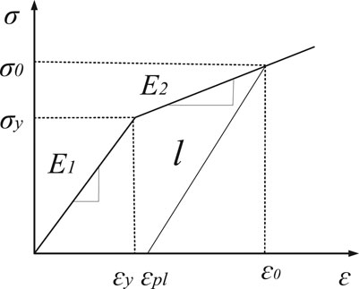
FIGURE 1. Stress and strain curves of the steel pipeline.

In case the longitudinal stress was less than the yield strength, the material characterizations were analyzed through a linear elasticity model. The maximum plastic strain of the analyzed material was considered 0.2%, The pipe will be failure when the material strain exceeds this value. Eq. 1 describes the stress-strain relationship of steel pipelines in an elastic-linear strain hardening model.

$\{\begin{array}{l}\sigma =E_1\epsilon \left(\epsilon \le {\epsilon }_y\right)\\ \sigma ={\sigma }_y+E_2\left(\epsilon -{\epsilon }_y\right)\left(\epsilon >{\epsilon }_y\right)\end{array}(1)$

Where $\sigma$ is the real stress in MPa. $\epsilon$ is the real strain. ${\sigma }_y$ is the yield strength of the analyzed material in MPa. E₁ and E₂ are the elastic and plastic modulus of the pipeline, respectively, in MPa.

The Pipe-Soil Interaction Model for Buried Pipelines

Eq. 2 describes the pipe-soil interaction as an ideal elastic-plastic model (Rajani et al., 1995).

$\{\begin{array}{l}f=\pi D{k}_{x}u\left(\left|u\right|\le u_x\right)\\ f=\pi D{k}_x{u}_x=F_x\left(\left|u\right|\ge u_x\right)\end{array}(2)$

Where f is the soil friction of pipes per unit length, u is the relative longitudinal displacement between pipe and soil, F_x is the ultimate soil resistance of pipes per unit length, and u_x is the longitudinal subgrade modulus of soil.

From Figure 2, the value of f was assumed to increase linearly with increasing the value of u when the relative longitudinal displacement value is smaller than the maximum elastic displacement. While the value of u reaches the maximum elastic displacement (i.e., u_x), the elastic stage of the soil enters the plastic state, and the value of f reaches the ultimate resistance and remains unchanged (i.e., F_x).

FIGURE 2

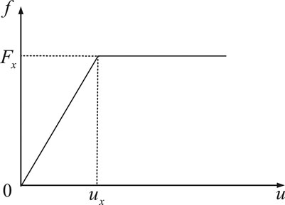
FIGURE 2. The pipe-soil interaction model (f: the soil friction of pipes per unit length; u: the relative longitudinal displacement between pipe and soil; F_x: the ultimate soil resistance of pipes per unit length; k_x: the longitudinal subgrade modulus of soil).

Analytical Method for the Longitudinal Strain of Pipelines

Mechanical Model

Figure 3 shows a side view of the pipeline sections subjected to the thawing landslide of soil. The section of BC was located in an unstable soil. Both sections of AB and CD were in stabilized soils. The length of the BC pipe section is L, and the slope angle is θ.

FIGURE 3

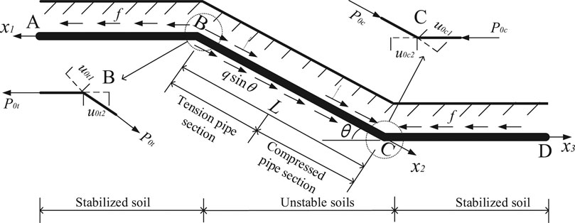
FIGURE 3. A side view of the pipeline sections subjected to the thawing landslide of soil.

The pipeline was mainly subjected to the axial force by soil slippage and friction force between pipeline and soil. As shown in Figure 3, the BC section of the pipeline was also subjected to gravity, which was expressed as $q\sin \theta$ alongside the axial direction. As found by the previous investigation results, the axial force of the pipeline in the slope section almost equals its horizontal section (Zhou, 2010). The axial displacement of the BC and AB sections at point B was $u_{0t1}$ and $u_{0t2}$, respectively, due to the axial tension$p_{0t}$. While the axial displacement of BC and CD sections at point C was $u_{0t1}$ and$u_{0t2}$, respectively, due to the axial compression $p_{0c}$.

According to the engineering, there is no relative displacement between the pipe and the soil when a pipe section is located in the unstable soil. Thus, the soil friction does not affect the pipeline. As shown in Figure 4, the axial force of the pipe reaches its maximum value at points B and C, and it gradually decreases to zero as it moves away from points B and C.

FIGURE 4

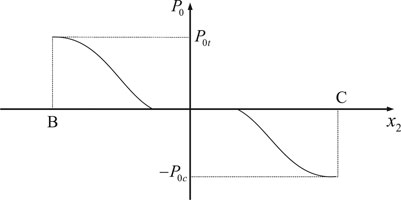
FIGURE 4. Distribution of axial force alongside the BC section of pipeline.

Considering the soil landslide, the axial force, P₀ (P_0t, P_0c), of the pipeline was calculated from Eq. 3.

$P_0=A\left({\sigma }_1^{total}-{\sigma }_1^{init}\right)(3)$

A is the cross-sectional area of pipeline in mm². ${\sigma }_1^{total}$ is the total longitudinal stress of the pipe in MPa. ${\sigma }_1^{init}$ is the initial axial force of pipeline in MPa due to the Poisson’ ratio and temperature effect, which was obtained from eq. (5) and (6).

${\sigma }_1^{init}=\nu {\sigma }_h-E_1\alpha \Delta T(4)$

${\sigma }_{\text{Mises}}=\sqrt{\frac{1}{2}\left[{\left({\sigma }_1-{\sigma }_2\right)}^2+{\left({\sigma }_2-{\sigma }_3\right)}^2+{\left({\sigma }_3-{\sigma }_1\right)}^2\right]}(5)$

From eq. (9) and (10), ${\sigma }_{Mises}$ is the Mises stress of pipeline.${\sigma }_1$, ${\sigma }_2$ and ${\sigma }_3$ are the maximum, intermediate, and minimum principal stresses of pipeline, respectively, in MPa. In this regard, the ${\sigma }_1$ of the pipeline is subjected to internal pressure, and the axial tensile load is the axial tensile stress. The ${\sigma }_2$ is the hoop stress ${\sigma }_h$ , while the ${\sigma }_3$ is 0. When the Mises stress value of the pipeline achieves the yield stress, it is considered to be yielded. The axial tensile stress ${\sigma }_{1y}^t$ was calculated from eq. (11) and (12) by considering the yield strength of the pipeline.

${\sigma }_{1y}^t=\frac{1}{2}\left({\sigma }_h+\sqrt{4{\sigma }_y^2-3{\sigma }_h^2}\right)(6)$

${\sigma }_h=\frac{p\left(D-2t\right)}{2t}(7)$

Similar to eq. (15) and (16), the ${\sigma }_1$ of the pipeline is subjected to the internal pressure, and the axial compression load is the hoop stress ${\sigma }_h$. The ${\sigma }_2$ is 0, and the ${\sigma }_3$ is the axial compression stress of the pipeline. The axial compression stress ${\sigma }_{1y}^c$ was calculated from eq. (17) by considering the yield strength of the pipeline.

${\sigma }_{1y}^c=\frac{1}{2}\left({\sigma }_h-\sqrt{4{\sigma }_y^2-3{\sigma }_h^2}\right)(8)$

Thus, the ultimate axial force of the pipeline was obtained from eq. (19) and (20) subjected to the tension and compression loads.

$P_{yt}=A\left({\sigma }_{1y}^t-{\sigma }_1^{init}\right)(9)$

$P_{yc}=A\left({\sigma }_{1y}^c-{\sigma }_1^{init}\right)(10)$

A vertical view of the pipeline crossing the slope is shown in Figure 5. The displacement of points A and D at the infinite far end of the horizontal pipeline is 0. The displacement at points B and C in the horizontal direction is converted into the slope direction. It was assumed that the displacement of the slope $u_{total}$ is equal to the geometric elongation of the pipe under a tension in the slope direction. It is also equal to the geometric compression of the pipe being compressed in the slope direction (eq. 23).

$\{\begin{array}{l}{u}_{total}\left(P_{0t}\right)=u_{0t1}\left(P_{0t}\right)+u_{0t2}\left(P_{0t}\right)\cos \theta \\ u_{total}\left(P_{0c}\right)=u_{0c1}\left(P_{0t}\right)+u_{0c2}\left(P_{0t}\right)\cos \theta \end{array}(11)$

FIGURE 5

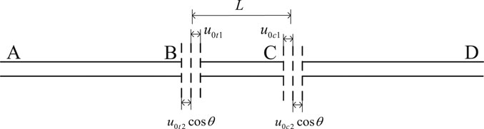
FIGURE 5. A vertical view of a pipeline longitudinally crossing a thawing landslide slope.

Governing Equations for a Pipe Segment in the Slope Section

As shown in Figure 5, the crossing pipeline in the slope was divided into three parts: AB ($-\infty \le x_1\le 0$), BC ($0\le x_2\le L$), and CD ($0\le x_3\le +\infty$) pipe sections. A micro-unit was selected from the section of BC in the pipeline. dx (x₁, x₂, and x₃) the length changes of the micro-unit, and N is the total axial force of the pipeline (Figure 6, eq. 25).

$N+\left(f+q\sin \theta \right)\cdot dx=N+dN(12)$

The density (${\rho }_{soil}=7.85\times {10}^{-6}kg/mm$) and gravity ($q={\rho }_{soil}D\pi t{g}_{gra}$) of the steel pipe are 2.49 kN/m and 77 kN/m, respectively. In this study, the friction force of the steel pipe is much greater than its gravity value; thus, the effect of gravity on the results was ignored (Eq. 13)-(15).

$N+f\cdot dx=N+dN(13)$

$\frac{dN}{dx}=\{\begin{array}{l}{k}_x\pi Du\text{When the soil is elastic}\\ F_x\text{When the soil is plastic}\end{array}(14)$

$\{\begin{array}{l}N=E_{1}A\epsilon =E_{1}A\frac{d}{dx}u\left(\epsilon \le {\epsilon }_y\right)\\ N=A{\sigma }_y+A{E}_2\left(\epsilon -{\epsilon }_y\right)=A{\sigma }_y+A{E}_2\left(\frac{d}{dx}u-{\epsilon }_y\right)\left(\epsilon >{\epsilon }_y\right)\end{array}(15)$

Eq. (30) and (31) were obtained through substituting the geometric eq. (32) and (33).

$\{\begin{array}{l}\frac{d^{2}u}{d{x}^2}-\frac{k_{x}u\pi D}{EA}=0\text{When the soil is elastic}\\ \frac{d^{2}u}{d{x}^2}-\frac{F_x}{EA}=0\text{When the soil is plastic}\end{array}(16)$

$\{\begin{array}{l}u=k_1{e}^{\lambda x_2}+k_2{e}^{-\lambda x_2}\text{When the soil is elastic}\\ u=\frac{1}{2EA}\hspace{0.17em}{F}_x{x}^2+k_{3}x+k_4\text{When the soil is plastic}\end{array}(17)$

Where $\lambda =\sqrt[2]{k_x\pi D/EA}$, $k_1$, $k_2$, $k_3$, $k_4$ are undetermined coefficients.

FIGURE 6

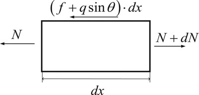
FIGURE 6. A schematic diagram of the total axial force in the pipeline segments.

The Distribution Function of the Longitudinal Strain in Pipelines

Pipelines in unstable and stabilized soils are semi-infinite (Xi and Wen, 2019), the tension section of the pipeline in the uphill stabilized and unsteady slope soils is symmetrical. Meanwhile, the compression section of the pipeline in the downhill stabilized and unsteady slope soils is symmetrical. The distribution function of the longitudinal strain in pipelines were divided into three stages I, II, and III.

At the stage I, the pipeline and soil represent an elastic state. As shown in Figure 7, the coordinate value of point B is 0. The soil on the left and right sides of point B is defined as stabilized and unstable types, respectively.

FIGURE 7

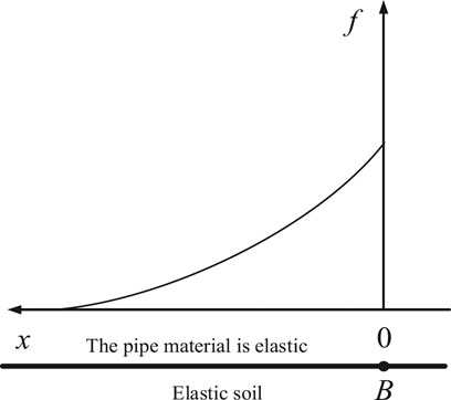
FIGURE 7. The distribution of soil reaction forces in the tension section of the pipeline at the stage I.

The displacement and strain functions of the uphill pipeline section were determined as follows:

$u_1=a_1{e}^{\lambda x_2}+a_2{e}^{-\lambda x_2}(18)$

${\epsilon }_1=a_1\lambda e^{\lambda x_2}-a_2\lambda e^{-\lambda x_2}(19)$

Where boundary conditions are $u_{1(x=+\infty )}=0$ and ${\epsilon }_{1(x=0)}=\frac{P_{0t}}{E_{1}A}$. Thus,

$u_1=-\frac{P_{0t}}{E_{1}A\lambda }\hspace{0.17em}{e}^{-\lambda x}(20)$

${\epsilon }_1=\frac{P_{0t}}{E_{1}A}\hspace{0.17em}{e}^{-\lambda x}(21)$

In eq. (40) and (41), the displacement of the horizontal section in the pipeline at point B is $u_{0t2}=\frac{P_{0t}}{E_{1}A\lambda }$. The displacement of the horizontal section in the pipeline at point C is $u_{0c2}=\frac{P_{0c}}{E_{1}A\lambda }$.

At the stage II, the soil is in a plastic state, and the pipeline is in a elastic state. As shown in Figure 8, the coordinate value of point B₁ is 0. When x ≤ 0, the soil is in an elastic state. When 0 < x ≤ L_BB1, the soil is in a plastic state.

FIGURE 8

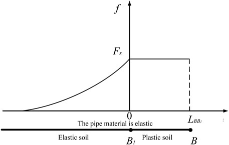
FIGURE 8. The distribution of soil reaction forces in the tension section of the pipeline at the stage II.

The displacement and strain functions of the uphill section of pipeline are as follows:

$\{\begin{array}{l}{u}_1=a_3{e}^{\lambda x}+a_4{e}^{-\lambda x}\left(-\infty <x\le 0\right)\\ u_1=\frac{1}{2EA}\hspace{0.17em}{F}_x{x}^2+a_{5}x+a_6\left(0\le x\le L_{B{B}_1}\right)\end{array}(22)$

$\{\begin{array}{l}{\epsilon }_1=a_3\lambda e^{\lambda x}-a_4\lambda e^{-\lambda x}\left(-\infty <x\le 0\right)\\ {\epsilon }_1=\frac{1}{EA}\hspace{0.17em}{F}_{x}x+a_5\left(0\le x\le L_{B{B}_1}\right)\end{array}(23)$

Where boundary conditions are $u_{1(x=-\infty )}=0$, $u_{1(x=0)}=u_x$, and ${\epsilon }_{1(x=L_{B{B}_1})}=\frac{P_{0t}}{E_{1}A}$.

$\{\begin{array}{l}{u}_1=u_x{e}^{\lambda x}\left(-\infty <x\le 0\right)\\ u_1=\frac{1}{2E_{1}A}{F}_x{x}^2+\frac{P_{0t}-F_x{L}_{B{B}_1}}{E_{1}A}x+u_x\left(0\le x\le L_{B{B}_1}\right)\end{array}(24)$

$\{\begin{array}{l}{\epsilon }_1=u_x\lambda e^{\lambda x}\left(-\infty <x\le 0\right)\\ {\epsilon }_1=\frac{1}{E_{1}A}\hspace{0.17em}{F}_{x}x+\frac{P_{0t}-F_x{L}_{B{B}_1}}{E_{1}A}\left(0\le x\le L_{B{B}_1}\right)\end{array}(25)$

Eq. (46) represents the displacement function of the horizontal section in the pipeline at point B.

$u_{0t2}=-\frac{1}{2E_{1}A}{F}_x{L}_{BB1}^2+\frac{P_{0t}}{E_{1}A}{L}_{B{B}_1}+u_x(26)$

$u_{0t2}=\frac{1}{2E_{1}A{F}_x}\left(P_{0t}^2-{\left(P_{0t}^{cril1}\right)}^2\right)+u_x(27)$

Also, the critical axial force and the displacement function at point C are formulated as eq. (49) and (50), respectively.

$P_{0c}^{cril1}=\left|-E_{1}S\lambda u_x\right|(28)$

$u_{0c2}=\frac{1}{2E_{1}A{F}_x}\left(P_{0c}^2-{\left(P_{0c}^{cril1}\right)}^2\right)+u_x(29)$

At the stage III, both the pipeline and soil are in a plastic state. As shown in Figure 9, the coordinate value of points B, B₂, and B₃ are $L_{B{B}_3}$, $L_{B_2{B}_3}$, and 0, respectively. When $x\le -L_{B_2{B}_3}$, the soil is in an elastic state. When $-L_{B_2{B}_3}<x\le -L_{B{B}_3}$, the soil is in a plastic state. Considering $x\le 0$ and $0<x\le -L_{B{B}_3}$, the pipeline is in an elastic and a plastic state, respectively. As the pipeline reaches $P_{0t}^{cri2}=P_{yt}$ at point B, the elastoplastic boundary is $P_{0\text{t}}=P_{yt}$. Also, the critical axial force of the pipeline is $P_{0t}^{cri2}$ at point B. When $P_{0\text{t}}>P_{yt}$ the pipeline enters a plastic state at point B. The length of the elastic section in the pipeline ($L_{B_2{B}_3}$) was calculated from eq. (53) in the plastic soil.

$L_{B_2{B}_3}=\frac{1}{F_x}\left(P_{0t}^{cril2}-P_{0t}^{cril1}\right)(30)$

At point B₃, the displacement function of the pipeline is:

$u_{0t3}=-\frac{F_x}{2E_{1}A}{L}_{B_2{B}_3}^2+\frac{P_{0t}^{cril2}}{E_{1}A}{L}_{B_2{B}_3}+u_x(31)$

Also, the length of the plastic section in the pipeline ($L_{B{B}_3}$) from eq. (56) in the plastic soil.

$L_{B{B}_3}=\frac{1}{F_x}\left(P_{0t}-P_{yt}\right)(32)$

Thus, the displacement and strain functions of the uphill horizontal section in the pipeline were calculated from eq. (58) and (59).

$\{\begin{array}{l}{u}_1=a_7{e}^{\lambda x}+a_8{e}^{-\lambda x}\left(-\infty <x\le -L_{B_2{B}_3}\right)\\ u_1=\frac{1}{2E_{1}A}{F}_x{x}^2+a_{9}x+a_{10}\left(-L_{B_2{B}_3}\le x\le 0\right)\\ u_1=\frac{1}{2E_{2}A}{F}_x{x}^2+a_{11}x+a_{12}\left(0\le x\le L_{B{B}_3}\right)\end{array}(33)$

$\{\begin{array}{l}{\epsilon }_1=a_7\lambda e^{\lambda x}-a_8\lambda e^{-\lambda x}\left(-\infty <x\le -L_{B_2{B}_3}\right)\\ {\epsilon }_1=\frac{1}{E_{1}A}{F}_{x}x+a_9\left(-L_{B_2{B}_3}\le x\le 0\right)\\ {\epsilon }_1=\frac{1}{E_{2}A}{F}_{x}x+a_{11}\left(0\le x\le L_{B{B}_3}\right)\end{array}(34)$

At the stage III, boundary conditions are ${\epsilon }_{1(x=L_{B{B}_3})}=\frac{P_{0t}}{E_{2}A}+\frac{P_{yt}}{E_{1}A}-\frac{P_{yt}}{E_{2}A}$, $u_{1(x=-\infty )}=0$, $u_{1(x=-L_{B_2{B}_3})}=u_x$, and $u_{1(x=0)}=u_{0t3}$.

$\{\begin{array}{l}{u}_1=u_x{e}^{\lambda L_{B_2{B}_3}}{e}^{\lambda x}\left(-\infty <x\le -L_{B_2{B}_3}\right)\\ u_1=\frac{1}{2E_{1}A}{F}_x{x}^2+\left(\frac{u_{0t3}-u_x}{L_{B_2{B}_3}}+\frac{F_x{L}_{B_2{B}_3}}{2E_{1}A}\right)x+u_{0t3}\left(-L_{B_2{B}_3}\le x\le 0\right)\\ u_1=\frac{1}{2E_{2}A}{F}_x{x}^2+\left(\frac{P_{yt}}{E_{1}A}-\frac{P_{yt}}{E_{2}A}\right)x+\frac{1}{E_{2}A}\left(P_{0t}-F_x{L}_{B{B}_3}\right)x+u_{0t3}\left(0\le x\le L_{B{B}_3}\right)\end{array}(35)$

$\{\begin{array}{l}{\epsilon }_1=u_x{e}^{\lambda L_{B_2{B}_3}}\lambda e^{\lambda x}\left(-\infty <x\le -L_{B_2{B}_3}\right)\\ {\epsilon }_1=\frac{1}{E_{1}A}{F}_{x}x+\frac{u_{0t3}-u_x}{L_{B_2{B}_3}}+\frac{F_x{L}_{B_2{B}_3}}{2E_{1}A}\left(-L_{B_2{B}_3}\le x\le 0\right)\\ {\epsilon }_1=\frac{1}{E_{2}A}{F}_{x}x+\frac{P_{yt}}{E_{1}A}-\frac{P_{yt}}{E_{2}A}+\frac{1}{E_{2}A}\left(P_{0t}-F_x{L}_{B{B}_3}\right)\left(0\le x\le L_{B{B}_3}\right)\end{array}(36)$

At point B, the displacement of the uphill horizontal section in the pipeline is:

$u_{0t2}=\frac{1}{2E_{2}A}{F}_x{L}_{B{B}_3}^2+\left(\frac{P_{yt}}{E_{1}A}-\frac{P_{yt}}{E_{2}A}\right)L_{B{B}_3}+\frac{1}{E_{2}A}\left(P_{0t}-F_x{L}_{B{B}_3}\right)L_{B{B}_3}+u_{0t3}(37)$

$u_{0t2}=\frac{P_{0t}^2}{2E_{2}A{F}_x}+\left(\frac{1}{E_2}-\frac{1}{E_1}\right)\frac{\left(P_{0t}^{cril2}-2P_{0t}\right)P_{0t}^{cril2}}{2A{F}_x}+\frac{u_x}{2}(38)$

At point C, the critical axial force ($P_{0c}^{cri2}=P_{yc}$) and the displacement function of the pipeline were calculated by the following equations.

$u_{0c2}=\frac{P_{0c}^2}{2E_{2}A{F}_x}+\left(\frac{1}{E_2}-\frac{1}{E_1}\right)\frac{\left(P_{0c}^{cril2}-2P_{0c}\right)P_{0c}^{cril2}}{2A{F}_x}+\frac{u_x}{2}(39)$

$u_{0t1}=u_{0t2};u_{0c1}=u_{0c2}(40)$

FIGURE 9

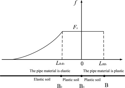
FIGURE 9. The distribution of soil reaction forces in the tension section of the pipeline at the stage III.

A Solution for the Maximum Longitudinal Strain of the Pipeline

The maximum longitudinal tensile strain of the pipeline is at point B, and the maximum longitudinal compressive strain is at point C. When the soil on the slope is in a plastic state, the friction force of the pipeline per unit length is F_x. The axial force of the pipeline at points B and C is $P_{0t}=P_{0t}^{\max }$ and$P_{0c}=P_{0c}^{\max }$, respectively. The equilibrium equation of axial force for the pipeline on the slope can be expressed as follows:

$P_{0t}^{\max }+P_{0c}^{\max }=F_{x}L(41)$

The amount of thawing landslide is the same on the uphill and downhill slopes. Thus, the maximum axial force of the pipeline and critical value of thawing landslide $u_s^{crit}$ is calculated using eq. (69) when the soil is in a plastic state.

$u_{total}\left(P_{0t}^{\max }\right)=u_{total}\left(P_{0c}^{\max }\right)(42)$

For a specific value of thawing landslide $u_s$, when $u_s<u_s^{crit}$, the soil is in an elastic state. Eq. (71) was used to calculate the axial force of the slope pipeline at points B and C.

$u_{total}\left(P_{0t}\right)=u_{total}\left(P_{0c}\right)=u_s(43)$

When $u_s\ge u_s^{crit}$, the soil is in a plastic state. The axial force of the slope pipeline at points B and C reaches the maximum value $P_{0t}=P_{0t}^{\max }$ and $P_{0c}=P_{0c}^{\max }$, respectively.

$\{\begin{array}{l}0<P_{0t}^{cril1}\left(\text{the first stage}\right)\\ P_{0t}^{cril1}\le P_{0t}\le P_{0t}^{cril2}\left(\text{the second stage}\right)\\ P_{0t}\ge P_{0t}^{cril2}\left(\text{the third stage}\right)\end{array}(44)$

$\{\begin{array}{l}0<P_{0c}^{cril1}\left(\text{the first stage}\right)\\ P_{0c}^{cril1}\le P_{0c}\le P_{0c}^{cril2}\left(\text{the second stage}\right)\\ P_{0c}\ge P_{0c}^{cril2}\left(\text{the third stage}\right)\end{array}(45)$

$\{\begin{array}{l}{P}_{0t}=E_{1}A{\epsilon }_B\left(\text{the first stage and second stage}\right)\\ P_{0t}=A{\sigma }_{yt}+A{E}_2^t({\epsilon }_B-{\epsilon }_{yt})\left(\text{the third stage}\right)\end{array}(46)$

$\{\begin{array}{l}{P}_{0c}=E_{1}A{\epsilon }_C\left(\text{the first stage and second stage}\right)\\ P_{0c}=A{\sigma }_{yc}+A{E}_2^c\left({\epsilon }_C-{\epsilon }_{yc}\right)\left(\text{the third stage}\right)\end{array}(47)$

The specific process is shown in Figure 10. The strain of the pipeline at points B and C are ${\epsilon }_B$ and ${\epsilon }_c$, respectively. Thus, the maximum longitudinal tensile and compressive strains of the pipeline can be expressed as eq. (77), respectively.

$\{\begin{array}{l}{\epsilon }_t^{\max }={\epsilon }_B+{\epsilon }_1^{init}\left(a\right)\\ {\epsilon }_c^{\max }={\epsilon }_C+{\epsilon }_1^{init}\left(b\right)\end{array}(48)$

FIGURE 10

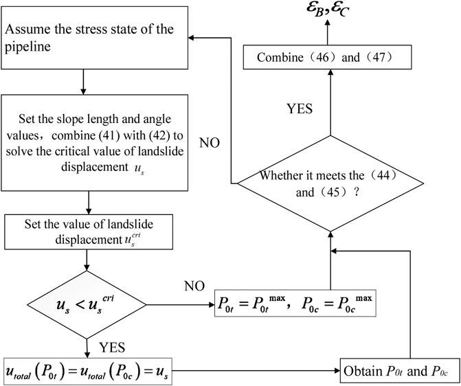
FIGURE 10. Steps for solving the maximum longitudinal strain of the pipeline at points B and C.

Validation of the Analytical Method

Verification of Strain Results Using Field Monitoring

To validate the developed analytical model, combined with the actual situation of an X65 pipeline in China, the analytical calculated results were compared with monitoring data. As shown in Supplementary Figure S2, the length of the slope is 1,000 m, and the slope angle is about 30°. The soil types mainly include silty clay, gravelly silty clay, gravel, and gravel sand. The value of a thawing landslide is about 10 mm. Table 1 represents the effective parameters of the pipeline subjected to the thawing landslide. The diameter (D) and the wall thickness (t) are 813 mm, 12.7 mm, respectively. Also, the design factor (f_p) is 0.4. Besides, the operating internal pressure (p) is 5.80 MPa, the yield strength of pipeline (σ_y), and the tensile strength (F_y) are 5.8, 450, and 535 MPa, respectively. The yield ratio (R_Y/T) and the Poisson’s ratio (v) are 0.84 and 0.3, respectively. Moreover, the elastic modulus (E₁) is 205 GPa, the plastic modulus ($E_2^t,E_2^c$) is 6,150 MPa. Furthermore, the temperature difference between the pipe installation and operation ($\Delta T$) is 20°C. The ultimate resistance of soil (F_x) is 77kN/m.

TABLE 1

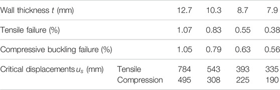
TABLE 1. Critical displacements of the thawing landslide of soil under an ultimate strain.

The stress value of the pipeline was obtained by a fiber grating sensing technology. The monitoring results revealed that the maximum longitudinal tensile stress at position 1 is 50 MPa, and the maximum longitudinal compressive stress at position 2 is 30 MPa. Theoretical calculation results showed that the maximum longitudinal tensile stress of the pipeline is 59.90 MPa, and the maximum longitudinal compressive stress is 35.55 MPa. The relative error between the analytical and monitoring results is less than 20%.

Verification via Previous Landslide FEM Results

To further validate the developed analytical model, a comparative analysis was performed between results from theoretical analysis of the maximum longitudinal strain and numerical simulation in the pipeline subjected to the thawing landslide of soil. Supplementary Table S1 represents the effective parameters of the pipeline subjected to the thawing landslide. Also, Figure 11 shows that the maximum longitudinal strain of the pipeline derived by the proposed analytical model agrees well with documented FE results.

FIGURE 11

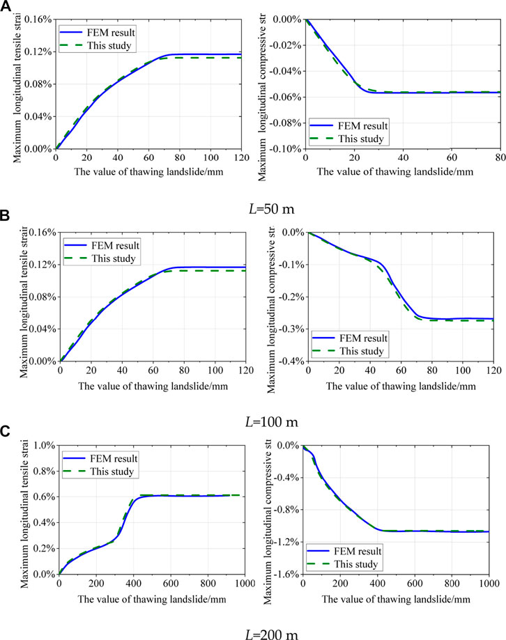
FIGURE 11. The result verification of the maximum longitudinal strain in the pipeline with (A) L = 50 m, (B) L = 100 m, and (C) L = 200 m.

Parametric Analysis of Pipes’ Maximum Longitudinal Strain

The maximum longitudinal strain subjected to thawing landslide was calculated by coding the program of the maximum longitudinal strain with numerical calculation software MATLAB. The size and operation related parameters, soil properties, and slope angle impact on the maximum axial strain of the pipeline subjected to thaw slumping load. In this section, the effects of wall thickness, internal pressure, ultimate resistance of soil, and slope angle are researched on the longitudinal strain of the pipeline.

Baseline Condition

Supplementary Table S2 shows basic parameters of the pipeline, which mainly come from the X65 pipeline in China. The slope length was ranged at 200, 300, 400, and 500 m, respectively. The calculated longitudinal tensile and compressive strains of the pipeline under the basic conditions are shown in Figure 12.

FIGURE 12

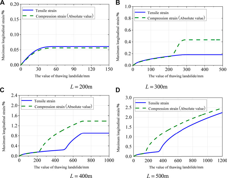
FIGURE 12. The maximum longitudinal strain of the pipeline under the reference condition with (A) L = 200 m, (B) L = 300 m, (C) L = 400 m and (D) L = 500 m.

From Figure 12, when the thermal melt slip of the soil reaches the critical value ($u_s^{cri}$), the frictional force between the pipeline and the soil reaches an ultimate resistance. It means the soil enters the plastic state, and the longitudinal strain of the pipeline also reaches the maximum value. As a result, the continuous increase of the slip will not cause the increase of the longitudinal strain.

The Ultimate Strain of the Pipeline

The tensile failure and compression buckling of the pipeline are related to each other. When the maximum longitudinal tensile strain reaches the ultimate tensile strain, the pipeline undergoes a tensile failure. While the maximum longitudinal compressive strain reaches the ultimate compressive strain, the compression buckling occurs in the pipeline. In this paper, the weld defect was assumed to be a surface type, and the strain-based design of CSA Z662-2007 guideline was used to calculate the ultimate tensile strain of the pipeline (eq. 49).

${\epsilon }_t^{cri}={\delta }^{\left(2.36-1.58R_{Y/T}-0.101\xi \eta \right)}\left(1+16.1R_{Y/T}^{-4.45}\right)\left(-0.157+0.239{\xi }^{-0.241}{\eta }^{-0.315}\right)(49)$

Also, a model proposed by CRES (Liu et al., 2017)which considered the critical compression factor comprehensively was adopted to calculate the ultimate compressive strain. This model accurately considers the geometrical imperfections and the pipeline properties (eqs. 50-58).

$F_{\text{LD}}=1(50)$

${\epsilon }_{\text{r}}=F_{\text{DP}}\cdot F_{\text{YT}}\cdot F_{\text{G}1}\cdot F_{\text{NF}}(51)$

$f_{\text{pc}}=1.8\times {10}^{-4}\times {\left(\frac{D}{\delta }\right)}^{1.6}(52)$

$f_{\text{p}}=\frac{PD}{2\delta {\sigma }_y}(53)$

$\{\begin{array}{l}{F}_{\text{DP}}=980\times \left[0.5{\left(\frac{D}{\delta }\right)}^{-1.6}+1.9\times {10}^{-4}\right]f_{\text{p}}<f_{\text{pc}}\\ F_{\text{DP}}=980\times \left(1.06f_{\text{p}}+0.5\right){\left(\frac{D}{\delta }\right)}^{-1.6}{f}_{\text{p}}\ge f_{\text{pc}}\end{array}(54)$

$f_{\text{g}}=\frac{h_g}{\delta }(55)$

$f_{\text{n}}=\frac{{\sigma }_{\text{a}}^{\text{c}}}{{\sigma }_{\text{y}}}(56)$

$\{\begin{array}{l}{F}_{\text{NF}}=1.2f_{\text{n}}^2+1f_{\text{n}}\ge 0\\ F_{\text{NF}}=1f_{\text{n}}<0\end{array}(57)$

${\epsilon }_{\text{c}}^{\text{crit}}=\min \left({\epsilon }_{\text{u}},F_{\text{LD}}\times {\epsilon }_{\text{r}}\right)(58)$

Supplementary Table S3 represents the results from the ultimate tensile strain parameters. The buckling strength ratio of the pipeline ($R_{\frac{Y}{T}}$) is 0.84, and the apparent toughness (${\delta }_T$) is 0.267 mm. By analyzing the factors affecting the tensile failure, the weld defect size is 50 × 5 mm. From analyzing the factors affecting the compression buckling, the peak wave of the weld defect from the height to bottom of the outer surface (h_g) is the maximum value of 0.13%D and 8%$\delta$.

The Effect of Wall Thickness

Due to different design factors of four regional levels, the wall thickness alongside the gas pipeline was different under the same design pressure. Figure 13 shows the effect of wall thickness on the pipeline’s maximum longitudinal tensile and compression strains. In Figure 13, the length of the slope is 500 m. The design factors are 0.4, 0.5, 0.6, and 0.72, and the internal pressure of the pipeline is set at 5.8 MPa. According to the specification of API standard steel pipe, the pipeline’s wall thickness is 12.7, 10.3, 8.7 and 7.9 mm, respectively. The values of other parameters are the same as shown in Supplementary Table S2.

FIGURE 13

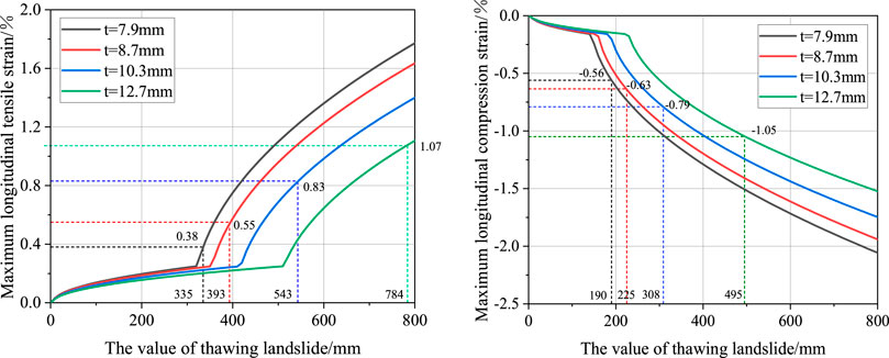
FIGURE 13. Influence of wall thickness on the maximum longitudinal strain.

As shown in Figure 13, the compression section of the pipeline is more likely to yield. As analyzed in Mechanical Model, the absolute value of the longitudinal compressive stress is less than the longitudinal tensile stress when the pipeline is yielding so that the stress of the pipeline is more likely to reach the yield stress under the compressional conditions. The pipeline is prone to a buckling damage at the bottom slope. These results are consistent with the actual situation in engineering (Randolph et al., 2010).

Both the maximum longitudinal tensile and compression strains increase with decreasing the pipe’s wall thickness. As indicated in Table 1, the smaller the pipe’s wall thickness leads to the smaller the critical displacement of soil. This is due to the fact that the smaller the wall thickness, the greater the hoop stress and the longitudinal strain of the pipeline. Moreover, a decrease in the ultimate tensile stress is due to the smaller of wall thickness. Therefore, the smaller the pipe’s wall thickness easily enters to the plastic state.

When the pipeline is in an elastic state, the wall thickness has little effect on the maximum longitudinal tensile and compression strains. In the pipe’s bilinear stress-strain model, the pipe’s elastic modulus is larger than the plastic modulus. Therefore, the fluctuation of longitudinal stress in the pipeline produces a larger strain change in the plastic state than the elastic state.

The Effect of Internal Pressure

The operating pressure alongside the pipeline was affected by seasonality and design factors. Figure 14 shows the effect of internal pressure on the maximum longitudinal tensile and compression strains of the pipeline. In Figure 14, the slope length and the wall thickness of the pipeline are 500 m and 12.7 mm, respectively. The design factor is 0.4, 0.5, 0.6, and 0.72. The internal pressure of the pipeline corresponds to 5.80, 7.26, 8.71, and 10.45 MPa, respectively. The values of other parameters are the same as shown in Supplementary Table S2.

FIGURE 14

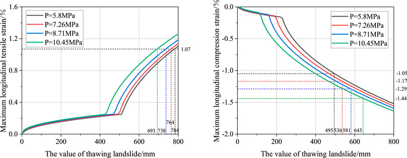
FIGURE 14. The effect of operating internal pressure on the maximum longitudinal strain.

As shown in Figure 14, both the maximum longitudinal tensile and compression strains of the pipeline increase with the internal pressure. Table 2 also represents the results of the critical displacement in the pipeline under various working conditions. The results show that the greater the internal pressure, the smaller the critical displacement of tensile failure. Due to the higher operating pressure of the pipeline, the hoop stress will be a larger value so that the longitudinal conduit of the strain increases. Pipes with larger internal pressure are more likely to achieve the yield strength under the same ultimate tensile strain. However, for compressive buckling case, the critical displacement increases with the internal pressure oppositely, caused by the increase of ultimate tensile strain.

TABLE 2

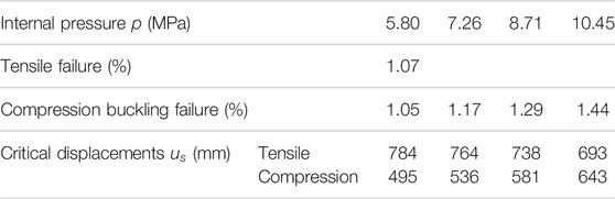
TABLE 2. The results of critical displacements in the thawing landslide of soil under an ultimate strain.

The Effect of the Maximum Resistance of Soil

The field investigation shows that the yielding soil displacement is between 5 and 8 mm; therefore, the ultimate resistance of the axial soil spring in the pipeline is between 77 kN/m and 122 kN/m. Figure 15 shows the effect of soil’s ultimate resistance on the maximum longitudinal tensile and compression strains in the pipeline. From Figure 15, the length of the slope is 500 m, the yielding soil displacement is between 5 and 8 mm, and the ultimate resistance of the soil per unit length is 77 kN/m, 92 kN/m, 107 kN/m, and 123 kN/m, respectively. The values of other parameters are the same as presented in Supplementary Table S2.

FIGURE 15

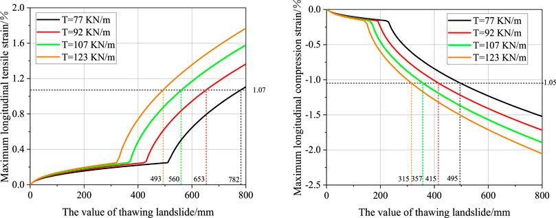
FIGURE 15. The effect of the maximum resistance of soil on the maximum longitudinal strain.

As shown in Figure 15, both the maximum longitudinal tensile and compression strains of the pipeline increase with the ultimate resistance of the soil. Table 3 also represents the results of the critical displacement in the pipeline under various working conditions. The results show that the greater the ultimate resistance of soil, the smaller the critical displacement of soil. Due to the greater the ultimate resistance of soil, the axial friction of the pipeline will be greater so that the greater the longitudinal strain is the easier the pipeline to achieve the yield strength.

TABLE 3

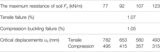
TABLE 3. The results of critical displacements of the thawing landslide of the soil under an ultimate strain.

The Effect of Slope Angle

The field investigation shows that most of the slope angles are between 20° and 60°. Figure 16 illustrates the effect of slope angle on the maximum longitudinal tensile and compression strains in the pipeline. From Figure 16, the length of the slope is 500 m, and the slope angle is between 20° and 60° with an equal interval of 5°. The values of other parameters are the same as presented in Supplementary Table S2.

FIGURE 16

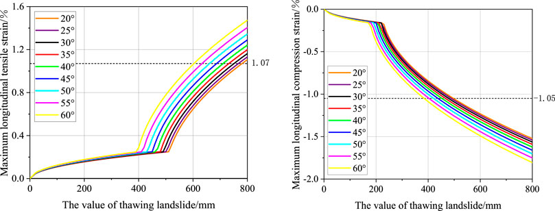
FIGURE 16. Influence of slope angle on the maximum longitudinal strain.

According to Figure 16, both the maximum longitudinal tensile and compression strains of the pipeline increase with the slope angle. Table 4 also represents the results of the critical displacement in the pipeline under various working conditions. The results show that the greater the slope angle, the smaller the critical displacement of soil. According to Figure 3. and Eq. (11), by increasing the slope angle ($\theta$), the value of $\cos \theta$ is smaller, and the axial force and the maximum axial strain are greater in the slope of pipeline, leading to easily achieve the yield strength.

TABLE 4

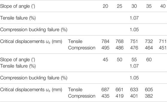
TABLE 4. The results of critical displacements of thawing landslide of soil under ultimate strain.

Conclusion

The purpose of the current study was to introduce an improved analytical method for the longitudinal strain analysis of buried pipelines subjected to the thaw slumping load. In the analytical calculations, a bilinear stress-strain model was adopted to the pipe material, and the pipe-soil interaction was assumed to be an ideal elastoplastic model. According to the elastoplastic change process of the pipeline-soil, the derivation was divided into three stages. First, the pipelines are all in the elastic state. Second, parts of the soil enter the plastic state, but the pipeline is still in the elastic state. Third, the pipeline and parts of the soil enter the plastic state. Based on these stages, the calculation method of the maximum longitudinal stress of the pipeline subjected to the thaw slumping load was given, and the rapid calculation of the maximum longitudinal strain of the pipeline was realized by numerical calculation software MATLAB. This research provides important insights into the improved analytical method is consistent with the calculated results of the nonlinear finite element model and is inconsistent with the real monitoring data of one X65 pipeline. Some conclusions can be drawn as follows:

1) In comparison with the tensile section, the compression section of the pipeline is more likely to yield. Since the absolute value of the longitudinal compressive stress is less than the longitudinal tensile stress, the pipeline is yielding so that the stress of the pipeline is more likely to reach the yield stress under a compressive condition. This result which discussed above is also consistent with the actual situation that the pipeline is prone to buckling damage at the bottom slope under pressure.

2) The maximum longitudinal tensile and compression strains decrease with the increase of wall thickness and increase with the internal pressure, the ultimate resistance of soil, and the slope angle. The soil’s ultimate resistance has the most significant influence on the maximum longitudinal strain, while the slope of angle has the most negligible impact.

3) The critical displacement of tensile failure in the pipeline increases with increasing the pipe’s wall thickness and decreases with increasing the internal pressure, the ultimate resistance of soil, and the slope angle. The main reason is that the hoop stress of the pipeline is closely related to the pipe’s wall thickness and operating internal pressure. The hoop stress increases as the pipe’s wall thickness decreases and the internal pressure increases, leading to increase the maximum longitudinal tensile strain. If the pipe’s wall thickness is smaller, the internal pressure is larger and the pipeline easily yields. While the ultimate resistance of soil increases and the slope angle decreases, the longitudinal tensile force and the maximum longitudinal tensile strain increases in the pipeline. It can be concluded that the larger ultimate resistance of soil leads to the smaller of slope angle and the pipeline easily yields.

4) The critical displacement of compressive buckling in the pipeline increases with increasing the pipe’s wall thickness and internal pressure; however, it decreases with increasing the ultimate resistance of soil and slope angle. The effect of the pipe’s wall thickness, the ultimate resistance of soil, and the slope angle on the critical displacement of compression buckling is the same as tensile failure effect on the pipeline. The ultimate compression stress increases with increasing the internal pressure, leading to an increase in the critical displacement of pipelines.

Data Availability Statement

The original contributions presented in the study are included in the article/Supplementary Material, further inquiries can be directed to the corresponding author.

Author Contributions

BJ: Research the method and wrote the first draft of the manuscrip XL: Methodological and theoretical guidance of the study DB: verify the method and data analysis YY and JJ: wrote sections of the manuscript YL: acquisition of data HZ: revising the manuscript critically for important intellectual content.

Funding

This research has been co-financed by National Science Foundation of China (Grant No. 52004314), Tianshan Youth Program (Grant No. 2019Q088), the Open Project Program of Beijing Key Laboratory of Pipeline Critical Technology and Equipment for Deepwater Oil and Gas Development (Grant No. BIPT2020005).

Conflict of Interest

Author DB was employed by company Western Pipeline Co. Ltd of PipeChina. Author YL was employed by company China Petroleum Pipeline Engineering Corporation.

The remaining authors declare that the research was conducted in the absence of any commercial or financial relationships that could be construed as a potential conflict of interest.

Publisher’s Note

All claims expressed in this article are solely those of the authors and do not necessarily represent those of their affiliated organizations, or those of the publisher, the editors and the reviewers. Any product that may be evaluated in this article, or claim that may be made by its manufacturer, is not guaranteed or endorsed by the publisher.

Supplementary Material

The Supplementary Material for this article can be found online at: https://www.frontiersin.org/articles/10.3389/fenrg.2021.742348/full#supplementary-material

References

Andrés, O., Hernandez, J., and Mauricio, P. O. (2017). Analysis and Mitigation Techniques for Axial Landslides to Pipeline: Case Study KM 35+690 Ocensa. ASME 2017 International Pipeline Geotechnical Conference, Lima, Peru, July 25-26, 2017.

Chan, P. (2000). Soil-Pipeline Interaction in Slopes. Canada: Doctoral dissertation, University of Calgary.

Chen, L. Q., Song, L. Q., Wu, X. D., Qiu, X. D., Liu, Q., Xia, Y., et al. (2017). Fem-based Stress Analysis of Gas Pipelines in Landslide Areas. Nat. Gas Industry.

Google Scholar

Chen, P. C. (2012). Risk Analysis and Management Solution in Permafrost Regions of Mohe-Daqing Pipeline. Pipeline Technique and Equipment. doi:10.3969/j.issn.1004-9614.2012.01.001

Chen, Q. Q., and Hu, M. L. (2014). Stress Analysis of Product Oil Pipeline Crossing Landslide Area. Pipeline Technique and Equipment. doi:10.3969/j.issn.1004-9614.2014.05.005

Eichhorn, G. N., and Haigh, S. K. (2018). “Landslide Pipe-Soil Interaction: State of the Practice,” in Pipeline Safety Management Systems; Project Management, Design, Construction, and Environmental Issues; Strain Based Design; Risk and Reliability; Northern Offshore and Production Pipelines, 2. doi:10.1115/ipc2018-78434

CrossRef Full Text | Google Scholar

Ho, D., Wilbourn, N., Vega, A., and Tache, J. (2014). Safeguarding a Buried Pipeline in a Landslide Region. Pipelines. 2014, 1162–1174. doi:10.1061/9780784413692.105

CrossRef Full Text | Google Scholar

Huang, K., Lu, H., Wu, S., Han, X., and Jiang, Y. (2015). The Stress Analysis of Buried Gas Pipeline Crossing the Landslide. Chin. J. Appl. Mech. 4, 689–693. doi:10.11776/cjam.32.04.D023

Google Scholar

Li, C., Ma, G., Cai, S., Yang, D., Xia, K., and Cui, H. (2016). Effect of Thawing Landslide on Stress of Buried Pipelines in Permafrost Regions. J. Liaoning Shihua Univ. 36, 30–33. doi:10.3969/j.issn.1672-6952.2016.03.007

Google Scholar

Liu, M., Zhou, H. G., and Wang, B. (2017). Strain-based Design and Assessment in Critical Areas of Pipeline Systems With Realistic Anomalies. TRB 2017 Meeting, Washington, DC.

Mcroberts, E. C., and Morgenstern, N. R. (1974). The Stability of Thawing Slopes. Can. Geotech. J. 11 (4), 447–469. doi:10.1139/t74-052

CrossRef Full Text | Google Scholar

O’Rourke, M. J., Liu, X., and Flores-Berrones, R. (1995). Steel Pipe Wrinkling Due to Longitudinal Permanent Ground Deformation. J. Transportation Eng. 121 (5), 443–451. doi:10.1061/(ASCE)0733-947x(1995)121:5(443)

CrossRef Full Text | Google Scholar

Rajani, B. B., Robertson, P. K., and Morgenstern, N. R. (1995). Simplified Design Methods for Pipelines Subject to Transverse and Longitudinal Soil Movements: Reply. Can. Geotechnical J. 32, 783. doi:10.1139/t95-111

CrossRef Full Text | Google Scholar

Randolph, M. F., Seo, D., and White, D. J. (2010). Parametric Solutions for Slide Impact on Pipelines. J. Geotech. Geoenviron. Eng. 136 (7), 940–949. doi:10.1061/(ASCE)gt.1943-5606.0000314

CrossRef Full Text | Google Scholar

Tsatsis, A., Kourkoulis, R., and Gazetas, G. (2015). Buried Pipelines Subjected to Ground Deformation Caused by Landslide Triggering, 5th ECCOMAS Thematic Conference. Comput. Methods Struct. Dyn. Earthquake Eng. 3, 25–27. doi:10.7712/120115.3524.1405

Google Scholar

Vasseghi, A., Haghshenas, E., Soroushian, A., and Rakhshandeh, M. (2021). Failure Analysis of a Natural Gas Pipeline Subjected to Landslide. Eng. Fail. Anal. 119, 105009. doi:10.1016/j.engfailanal.2020.105009

CrossRef Full Text | Google Scholar

Wang, L. W., Zhang, L., Dong, S. H., and Lu, M. X. (2014). Analysis of Mechanical Influencing Factors of Pipeline Landslide Based on Soil spring Model. Oil & Gas Storage Transport. 33, 380–390. doi:10.6047/j.issn.1000-8241.2014.04.008

Google Scholar

Xi, S., and Wen, B. P. (2019). Mechanical Response of Polygonal-Shape Transverse Buried Gas Pipeline Under the Action of Landslide. Oil & Gas Storage Transport. 38, 1350–1358. doi:10.6047/j.issn.1000-8241.2019.12.005

Google Scholar

Xu, X. Z., Wang, J. C., and Zhang, L. X. (2010). Frozen Soil Physics. Beijing: Science Press.

Yoosefghodsi, N., Zhou, J., and Murray, D. W. (2008). A Simplified Model for Evaluating Strain Demand in a Pipeline Subjected to Longitudinal Ground Movement. International Pipeline Conference, Calgary, September 29-October 3, 2008.

Yuan, Z. M. (1993). The Axial Force Caused by Landsliding Along the Axial Direction of Pipeline. Pet. Plann. Eng. 4, 35–38. doi:10.3969/j.issn.1004-2970.1993.06.006

Google Scholar

Zhang, H., and Liu, X. B. (2017). Design Strain Calculation Model for Oil and Gas Pipelines Subject to Geological Hazards. Oil & Gas Storage Transport. 36, 91–97. doi:10.6047/j.issn.1000-8241.2017.01.012

Google Scholar

Zhang, S. Z., Li, S. Y., Chen, S. N., Wu, Z. Z., Wang, R. J., and Duo, Y. Q. (2017). Stress Analysis on Large-Diameter Buried Gas Pipelines under Catastrophic Landslides. Pet. Sci. 14, 1-7. doi:10.1007/s12182-017-0177-y

CrossRef Full Text | Google Scholar

Zhou, W. (2010). Reliability of Pressurised Pipelines Subjected to Longitudinal Ground Movement. Struct. Infrastructure Eng. 8, 1–13. doi:10.1080/15732479.2010.505244

CrossRef Full Text | Google Scholar