Potential Analysis of the Attention-Based LSTM Model in Ultra-Short-Term Forecasting of Building HVAC Energy Consumption

Predicting system energy consumption accurately and adjusting dynamic operating parameters of the HVAC system in advance is the basis of realizing the model predictive control (MPC). In recent years, the LSTM network had made remarkable achievements in the field of load forecasting. This paper aimed to evaluate the potential of using an attentional-based LSTM network (A-LSTM) to predict HVAC energy consumption in practical applications. To evaluate the application potential of the A-LSTM model in real cases, the training set and test set used in experiments are the real energy consumption data collected by Kitakyushu Science Research Park in Japan. Pearce analysis was first carried out on the source data set and built the target database. Then five baseline models (A-LSTM, LSTM, RNN, DNN, and SVR) were built. Besides, to optimize the super parameters of the model, the Tree-structured of Parzen Estimators (TPE) algorithm was introduced. Finally, the applications are performed on the target database, and the results are analyzed from multiple perspectives, including model comparisons on different sizes of the training set, model comparisons on different system operation modes, graphical examination, etc. The results showed that the performance of the A-LSTM model was better than other baseline models, it could provide accurate and reliable hourly forecasting for HVAC energy consumption.

Introduction

According to statistics, building energy consumption accounts for about 40% of the total energy consumption (Mohsin et al., 2020), and the proportion of building carbon dioxide emissions is as high as 36% of the total emissions (Jradi et al., 2017; Mohsin et al., 2021). Heating, ventilation, and air-conditioning (HVAC) systems account for 40% (or even higher) of the commercial building energy consumption (Kim et al., 2019; Wang et al., 2021). Higher energy consumption usually means greater energy saving potential, so the research of energy-saving technology combining big data and artificial intelligence has become one of the hot spots in recent years (Sun et al., 2021). Simulation modeling is mainly used to predict energy consumption in the design stage of HVAC. The factors considered include building physical parameters, outdoor meteorological parameters, indoor environmental parameters, and room usage (Ma et al., 2017). Since there are different degrees of assumptions and simplifications in the process of establishing the model, there may be a large error between the predicted energy consumption in the design stage and the actual operation time. The data-driven forecasting model is mainly used to predict energy consumption in the operation stage of HVAC. The HVAC energy consumption is affected by many factors, not only by the building itself, but also by meteorological conditions (such as outdoor temperature and illumination), internal personnel activities (such as occupancy and power consumption), time lag, and the actual use of air conditioning (such as control deviation and operation scheme adjustment) (Wang et al., 2016). Under the influence of these factors, the HVAC load curve has the characteristics of strong fluctuation, large randomness, and not obvious periodicity compared with the electric load curve. This presents great challenges in designing data-driven HVAC models. To solve this problem, Wasim Iqbal et al. proposed the method of negative Binomial regression (NBR) model analysis (Iqbal et al., 2021), BinbinYu proposed a method based on the Dynamic Spatial Panel Model (DSPM) Model (Yu, 2021), and WeiqingLi et al. proposed the data envelopment analysis (DEA) and entropy method (Li et al., 2021a) to analyze the interaction between various factors. At present, the operating parameters of the HVAC system in buildings are mainly set according to the load prediction in the design stage. It will lead to the HVAC system working in a state of low efficiency, resulting in a large amount of energy consumption.

To solve this problem, Model predictive control (MPC) was proposed and had been widely used (Mayne, 2014; Sultana et al., 2017; Zhan and Chong, 2021). There have been many examples of load forecasting applied to MPC in other energy fields. For example, Xueyuan Zhao proposed a short-term household load forecasting model to guide users’ power consumption behavior and adjust power grid load (Zhao et al., 2021); Based on the forecast of wind power generation and electricity price, J.J. Yang proposed a charge-discharge control strategy for energy storage equipment based on the data drive, which realized the maximization of income of energy storage equipment (Yang et al., 2020a). Fangyuan Chang proposed a charging cost control solution based on reinforcement learning by using long and short-term memory networks (LSTM) to predict real-time electricity prices (Chang et al., 2020). Jin Li proposed an adaptive genetic algorithm based on neighborhood search to optimize the total cost related to energy consumption and running time of electric vehicles. (Li et al., 2020). This shows that predicting system energy consumption accurately and adjusting dynamic operating parameters of the HVAC system in advance is the basis of realizing MPC (Hazyuk et al., 2012).

Load forecasting can be divided into ultra-short-term, short-term, medium-term, and long-term according to different purposes, and the ultra-short-term load forecast refers to the load forecast within 1 h in the future (Guo et al., 2018; Qian et al., 2020). Due to the time delay of building thermal load, the change of influencing factors in the short term cannot immediately change the HVAC energy consumption (Huang and Chow, 2011). Therefore, the prediction of ultra-short-term load can minimize the impact of the uncertainty of input variables on the prediction results. The behavior of HVAC can be expressed as time-series data with a certain periodically. The prediction model can learn the load mode of the system from the time-series data, and use these modes to make load predictions. After the prediction range is determined, the appropriate algorithm needs to be selected. The algorithms in the field of time series prediction can be divided into two categories: traditional machine learning algorithms and deep learning algorithms. Traditional machine learning algorithms are mostly based on statistical models, Current popular algorithms include Autoregressive Moving Average (ARIMA) (Liu et al., 2021), support vector machine (SVM) (Ma et al., 2018), Regression Tree (Yang et al., 2020b), Random Forest (Li et al., 2021b), and artificial neural networks (ANN) (Wei et al., 2019; Bui et al., 2020).

In recent years, with the rapid development of deep learning, the deep neural network has been more and more applied in the field of load prediction. Deep learning is a series of new structures and new methods evolved based on multi-layer neural networks (Lv et al., 2021a). Deep learning models have obvious advantages over traditional machine learning models in predicting multivariable time series problems. In the real world, time series prediction presents multiple challenges, such as having multiple input variables, the need to predict multiple time steps, and the need to perform the same type of prediction for multiple actual observation stations (Askari et al., 2015). In particular, a deep learning model can support any number but a fixed number of inputs and outputs. Multivariable time series have multiple time-varying variables, each of which depends not only on its past value but also on other variables. These characteristics are correlated with each other, and in this case, multiple variables need to be considered to give the best-predicted energy consumption.

The most basic Deep learning model is Deep Neural Networks (DNN), also known as multi-layer perceptron (MLP). DNN has more hidden layers than ordinary artificial neural networks, which gives it the ability to learn complex patterns. Deb proposed a DNN - based model for predicting the daily cooling load of buildings (Deb et al., 2016). Massana proposed a DNN model-based method for predicting short-term electrical loads in non-residential buildings (Massana et al., 2015). Zhihan Lv et al. proposed a layered DAE support vector machine (SDAE-SVM) model based on a three-layer neural network and achieved good prediction results (Lv et al., 2021b). However, the DNN model cannot retain time-series information. It can only be predicted according to the current input and output values, and cannot learn the time dependence of data, which limits the accuracy of its prediction time series.

Recursive neural network (RNN), as a special deep neural network, can retain and consider the time variation of time series in the training process (Hochreiter and Schmidhuber, 1997), which makes it very suitable for time series data with periodicity. The time series of HVAC energy consumption is influenced by environmental variables and human living habits and has a strong periodicity. However, due to the problems of gradient explosion and gradient disappearance in the RNN network, the long-term dependence in time series cannot be retained, which limits the prediction accuracy of the RNN network. The long-short term memory (LSTM) network adds a series of multi-threshold gates based on the RNN network, which can deal with a long-term dependency relationship to a certain extent. LSTM networks were first used in natural language processing (Verwimp et al., 2020), machine translation (Su et al., 2020) and video recognition (Lv et al., 2021c), etc. In recent years, LSTM networks have attracted more and more attention in the field of load prediction. The authors of (Wang et al., 2019a) used the LSTM network to build a regional scale building energy consumption prediction model. Sendra-Arranz proposed a variety of multi-step prediction models based on the LSTM network to predict residential HVAC consumption (Sendra-Arranz and Gutiérrez, 2020). Zhe Wang proposed a new method for predicting plug loads using the LSTM network. Through the data collected from a real office building in Berkeley, California, the prediction accuracy of this method was verified to be better than that of the traditional machine learning algorithm (Wang et al., 2019b; Wang et al., 2020).

Since the LSTM network adopts the code-decoding framework, the limitations of the code-decoding framework will lead to information loss when processing long time series. Bahdanau first introduced the attention mechanism into the code-decoding framework in 2014 (Bahdanau et al., 2014). The attention mechanism can quantitatively assign a weight to each specific time step in the time series feature, which improves the attention distraction defect of traditional LSTM (Li et al., 2019). As far as the author knows, the LSTM model based on the ATTENTION mechanism has not been applied in the field of HVAC energy consumption prediction, but some researchers have started experiments in other load fields and achieved some results (Lu et al., 2017; Yu et al., 2017; Liang, et al, 2018). Such as Heidari used an attention-based LSTM (A-LSTM) model to predict the load of the solar-assisted hot water system and proved that the prediction accuracy of the A-LSTM model was better than that of the traditional LSTM model (Heidari and Khovalyg, 2020). Jince Li proposed an improved attention-based LSTM (A-LSTM) model for multivariate time series of predictions of two process industry cases (Li, et al, 2021c). Tongguang Yang proposed an attention-based LSTM model to predict the day-ahead PV power output (Yang et al., 2019). All these cases show that the A-LSTM model has significant advantages over the traditional LSTM model in dealing with time series problems.

This paper aims to develop a new HVAC ultra-short-term energy consumption prediction model. To achieve this goal, this paper first conducted potential rule analysis and feature engineering for 9 years’ operation data of Kitakyushu Science and Research Park’s (KSRP) Energy Center and constructed a data set for modeling. Then, we developed the LSTM model based on this data set and developed the A-LSTM model by adding the attention layer to the LSTM model. Besides, the RNN model, DNN model, and SVR model were also developed to compare performance. The hyper-parameters of the above models were optimized by the TPE algorithm to ensure prediction accuracy. Next, we used the data from the Energy Center from 2002 to 2009 as the training set and the data from 2010 as the test set to conduct experiments, and gradually reduced the size of data sets to evaluate the performance of the above five models in different training sets. Finally, we also evaluated the small-scale prediction effects of the above five models under four typical operating modes.

Based on the literature review the main novelty of the paper can be summarised as follows:

• This paper studies and verifies that the deep learning method with the attention mechanism has advantages in the memory and feature selection of time series information of air conditioning load prediction. As far as the author knows, the LSTM model based on the ATTENTION mechanism has not been applied in the field of HVAC energy consumption prediction.

• In this paper, we use the Tree-Structured of Parzen Estimators (TPE) algorithm to optimize the parameters of each baseline model, to ensure that all the baseline models involved in horizontal comparison are in the best prediction performance, and to ensure the authenticity of the prediction performance comparison

• In this paper, we used the real building data set instead of the standard data set to verify the load prediction potential of the A-LSTM model, which verified the value of this model in actual engineering. The results show that the A-LSTM model has advantages over the traditional machine learning algorithm in various operating modes, especially in the heating high load period, and has great potential in the field of ultra-short-term load prediction of HVAC.

Methodology

LSTM Neural Network

RNN network is a kind of neural network used to process time series. Compared with the traditional DNN network and CNN network, RNN adopts a cyclic structure to replace the hidden layer of the feedforward neural network. In the process of information transmission, there will be a part of the information left in the current neuron during each cycle, and the retained information will be used as the input of the next neural unit with the new information. In this way, the RNN network implements “memory”. However, when the input time series is too long, it is difficult to retain the information in the RNN network, this is also known as the phenomenon of gradient disappearance and gradient explosion (Hochreiter and Schmidhuber, 1997).

Based on the RNN unit, the input gate $i_t$, output gate $o_t$, forgetting gate $f_t$ and cell state $C_t$ are added to the LSTM unit to control the inheritance and abandonment of information. There are three inputs of the LSTM unit: the input vector $x_t$ at the current time slot t, the unit state $C_{t-1}$ at the time slot t−1, and the state of the hidden layer $h_{t-1}$ at the time slot t−1. The final output of the LSTM unit is the cell state $C_t$ at the current time slot t and the state of the hidden layer at the current time $h_t$ To figure out the $h_t$, we first let the $W_i,W_o$ and $W_f$ be the weight matrix of the input gate, the output gate, and the forgetting gate, and let the $\left[h_{t-1},x_t\right]$ represent the combination of the hidden state at the moment t−1 and the input of the unit at the time slot t into a new vector. Besides, let the $b_i$, $b_o$, and $b_f$ be their bias vectors, and let the $\sigma$ represent the Sigmoid activation function. The formulas of the $i_t$, $o_t$, and $f_t$ are shown below:

$i_t=\sigma \left(W_i\cdot \left[h_{t-1},x_t\right]+b_i\right)(1)$

$o_t=\sigma \left(W_o\cdot \left[h_{t-1},x_t\right]+b_o\right)(2)$

$f_t=\sigma \left(W_f\cdot \left[h_{t-1},x_t\right]+b_f\right)(3)$

Finally, let $\text{tan}h$ represent the activation function, $\text{*}$ represent the Hadamard product, and let the ${\tilde{C}}_t$ be the state of the intermediate unit input at time slot t, then we can calculate the $h_t$ as follows:

${\tilde{C}}_t=\text{tan}h\left(W_C\cdot \left[h_{t-1},x_t\right]+b_c\right)(4)$

$C_t=f_t\ast C_{t-1}+i_t\ast {\tilde{C}}_t(5)$

$h_t=o_t\ast \text{tan}h\left(C_t\right)(6)$

Attention Mechanism

Although the LSTM model has a memory function, and it can save some time-series information, but because the standard LSTM model uses the traditional encoder-decoder structure, it still has some limitations. When processing the time series $x_t$, the Encoder will first encode the input sequence into a fixed-length implicit vector $h$ and give the same weight to the implicit vector. However, when the length of $x_t$ increases, the average weight distribution will reduce the discrimination of $x_t$, and some important time-series information will be ignored in the process of training the model, thus affecting the prediction accuracy of the model.

The Attention mechanism is a mechanism used to optimize the Encoder-Decoder structural model, It can be combined with a variety of models depending on the actual situation. An encoder-decoder model with an Attention mechanism first learns the weight of each element from the sequence and then recombines the elements by weight. By assigning different weight parameters to each input element, the Attention mechanism can focus more on the parts that are relevant to the input element, thereby suppressing other useless information. Its biggest advantage is that it can consider global connection and local connection in one step, and can realize the parallel computation, which is particularly important for big data computation. In this paper, the Bahdanau algorithm (Bahdanau et al., 2014) is adopted to realize the Attention mechanism, and the structure of the A-LSTM model adopted is shown in Figure 1:

FIGURE 1

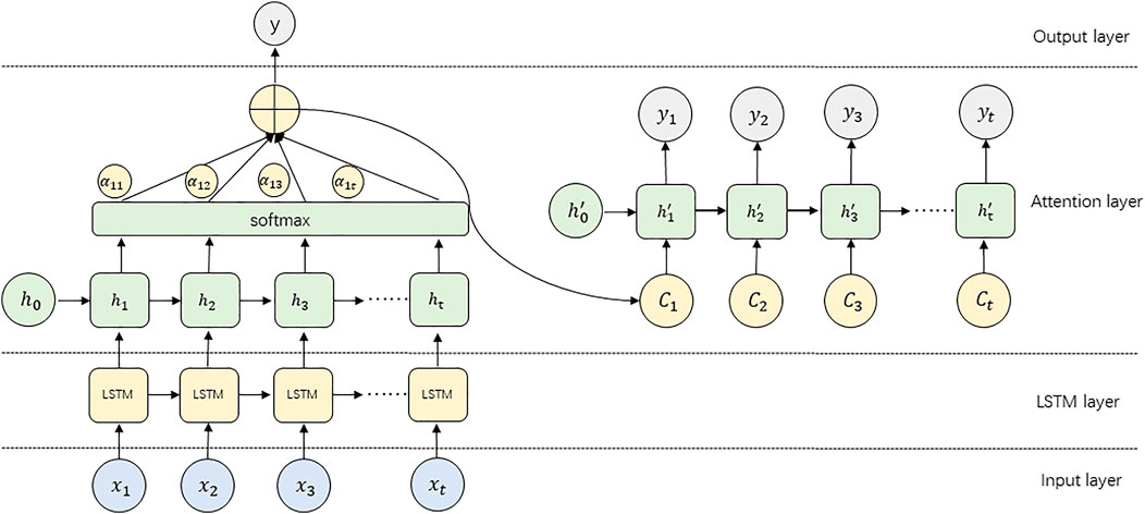
FIGURE 1. The structure of the A-LSTM model.

The calculation process of the Attention layer is shown in Eqs 7–9. $\text{i}$ denotes the moment; $j$ denotes the j element in the sequence; $T$ denotes the length of the sequence; ${\alpha }_{tj}$ denotes the weight value; $e_{tj}$ is the matching degree between the element to be encoded and other elements.

$e_{tj}=a\left(h_{i-1},h_j\right)(7)$

${\alpha }_{tj}=\frac{\exp \left(e_{tj}\right)}{{\Sigma }_{k=1}^t\exp \left(e_{tj}\right)}(8)$

$C_t={\displaystyle \sum }_{j=1}^T{\alpha }_{tj}{h}_i(9)$

Tree-Structured of Parzen Estimators

The performance of machine learning models largely depends on the selection of hyperparameters. With the increase of model complexity and the amount of training data, automatic hyperparameter optimization plays an increasingly important role in the developments (Nguyen et al., 2020). Compared with traditional manual parameter adjustment, automatic parameter optimization has the following advantages: 1) It reduces the manpower of development work. 2) Improve the performance of machine learning models. 3) Improve the reproducibility of the results (Luo et al., 2021). In this paper, the Tree-Structured of Parzen Estimators (TPE) algorithm was used to achieve automatic optimization of the model’s hyperparameters. TPE algorithm is an improved algorithm of Bayesian optimization algorithm (BO). It solves the limitation of the traditional BO algorithm to deal with classification parameters and conditional parameters, so it has higher efficiency.

The main process of the TPE algorithm is to convert the hyperparametric space into the nonparametric density distribution first, and then model the process $p\left(x|y\right)$. As shown in Eq. 10, TPE uses two density distributions of Equation to define $p\left(x|y\right)$, $y<y^{\text{*}}$ indicates that the value of the objective function is less than the threshold, and $y\ge y^{\text{*}}$ denotes that the value of the objective function is greater than or equal to the threshold.

$p\left(x|y\right)=\{\begin{array}{c}l\left(x\right) \text{if} y<y^{\ast }\\ g\left(x\right) \text{if} y\ge y^{\ast }\end{array}(10)$

The calculation of Expected Improvement (EI) is shown in Eqs 11–13.

$E\left(x\right)=\underset{-\infty }{\overset{y^{\ast }}{{\displaystyle \int }}}\left(y^{\ast }-y\right)\frac{p\left(x|y\right)p\left(y\right)}{p\left(x\right)}\text{d}y(11)$

$\gamma =p\left(y<y^{\ast }\right)(12)$

$P\left(x\right)=\underset{R}{{\displaystyle \int }}P\left(x|y\right)P\left(y\right)\text{d}y(13)$

Substitute Eqs 12, 13 into Eq. 11 to get the final Eq. 14.

$E{I}_{y^{\ast }}\left(x\right)={\left(\gamma +\frac{g\left(x\right)}{l\left(x\right)}\left(1-\gamma \right)\right)}^{-1}(14)$

It can be seen from Eq. 13 that point $x^{\text{*}}$ with the largest Ei is the point with the smallest $g\left(x\right)/l\left(x\right)$. The TPE algorithm evaluates the improvement points according to $g\left(x\right)/l\left(x\right)$ in each iteration, and finally returns a point $x^{\text{*}}$ with the largest EI. The corresponding process is shown in Figure 2.

FIGURE 2

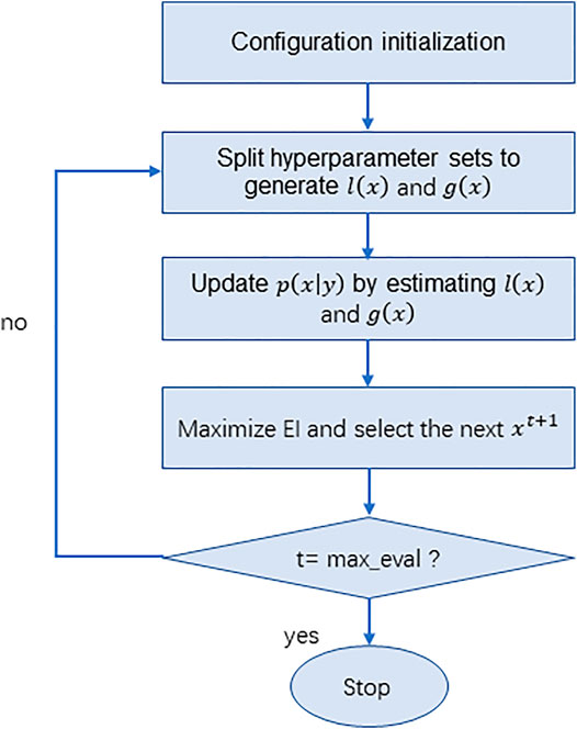
FIGURE 2. Flowchart of the TPE algorithm.

Case Study

Case Introduction

In this paper, data collected by the CCHP system of Kitakyushu Science Research Park (KSRP) in Japan were used as the research object. The KSRP system was a distributed energy system consisting of a gas engine (160 kW), a fuel cell (200 kW), and a photovoltaic system (150 kW). The system mainly supplied energy to the main teaching building of The University of Kitakyushu, which can meet the teaching and office needs of more than 3,000 people. The target building was divided into four floors, the first floor included the student center, meeting rooms and classrooms. The second to fourth floors were teachers’ offices and student research rooms.

The system was powered by the gas engine, fuel cells, photovoltaic system and the utility grid. The cooling load, heating load and hot water load were mainly provided by the absorption chiller, while the gas engine and fuel cell also provided part of the cooling and heating load when generating electricity. The basic schematic diagram of CCHP system at KSRP was shown in Figure 3. The system also included a detailed data acquisition system that recorded not only detailed operational data for each device, but also environmental data related to the target building. Using the temperature and flow data collected by the data acquisition system for hot and cold water supply and recovery, we could calculate the hot and cold load requirements of the target building in real-time. The KSRP cogeneration system was established in 2001. To make the model reflect the most real operating state of the system, we selected the data from 2002 to 2010 as the research object (78,820 pieces of data), because only 3 days of system failure occurred during this period, which could reduce the impact of data missing on the modeling.

FIGURE 3

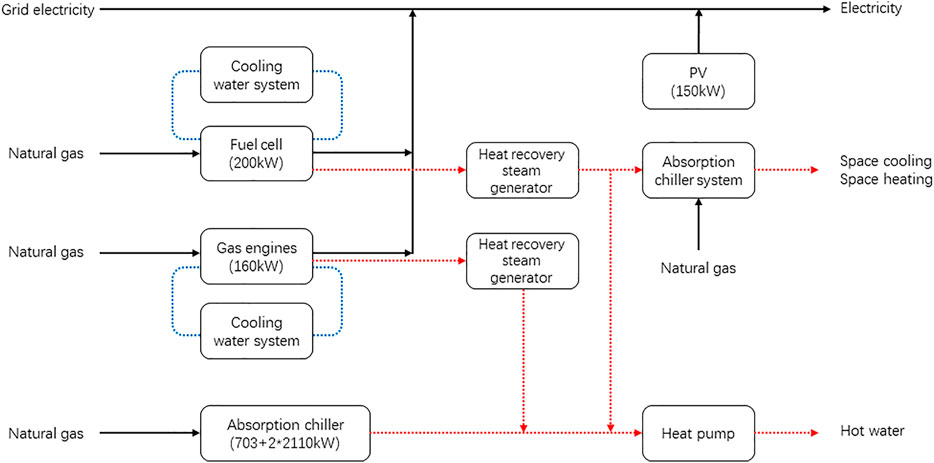
FIGURE 3. The basic schematic diagram of the CCHP system at KSRP.

Potential Analysis of Input Data Set

We first calculated the cooling and heating output of the equipment from January 1, 2002, to December 31, 2010, based on the gas consumption of the equipment and the annual average COP(cooling 1.00, heating 0.85). To verify the authenticity of the data, we also calculated the cooling and heating output based on the temperature and flow rate of cold and hot water supply and recovery collected by the system. To explore the distribution rule of these data in time series, we calculated the mean value of load in units of the month, week and hour respectively, and the results are shown in Figure 4. As can be seen from Figure 4A, the average load varies greatly each month. The annual peak value of total heating load output occurs in January, and that of total cooling load output occurs in August. Therefore, December, January, February, and March were defined as the heating season; July, August, and September as the cooling season; April, May, June, October, and November as the low-load season. The prediction effect of the model will be evaluated respectively according to this division. It can be seen from Figure 4B that the cooling and heating loads are higher on weekdays than on weekends; It also can be seen from Figure 4C that the average daily load distribution in the heating season and the cooling season is significantly different. All of the above time information can reflect the impact of human activities on load, so they can be used as characteristic factors for database construction.

FIGURE 4

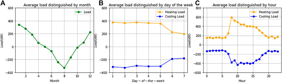
FIGURE 4. The diagram of average load distributed by the time: (A) average load distinguished by month, (B) average load distinguished by day of the week, (C) average load distinguished by hour.

We also selected other environmental factors that might affect the heat and cold output to build the initial database, including data collected by the Energy Center every hour from January 1, 2002, to December 31, 2010, a total of 78,820 pieces of data. Each group of data includes time information, outdoor temperature (°C), relative humidity (%), irradiance ($W\mathrm{∕}{m}^2$), wind speed (m/s), wind direction, and load output (The positive load indicates the heating load, and the negative load indicates the refrigeration load). In addition, the index “trend” indicates the ordinal number of the data in the time series. Since features with small correlation will provide unnecessary information in the training of the model, which will affect the robustness of the model, Pearson correlation analysis was conducted for all features, and the results are shown in Figure 5. It can be seen that the biggest factor affecting the load is outdoor temperature, followed by the time serial number. The correlation between wind direction and load was too small (−0.0087), and we had deleted this feature in later modeling. Examples of these data were shown in Table 1. In the following experiments, we used the data from 2002 to 2009 as the training set, the data from 2010 as the test set, and then randomly extracted 20% data from the training set as the verification set. Since the numerical dimensions of different variables are greatly different, it is necessary to normalize the data so that the data can be uniformly mapped to the interval [0,1]. In the next section, based on this data set, we will build a prediction model that can predict the next hour’s load according to the input data of the first N hours.

FIGURE 5

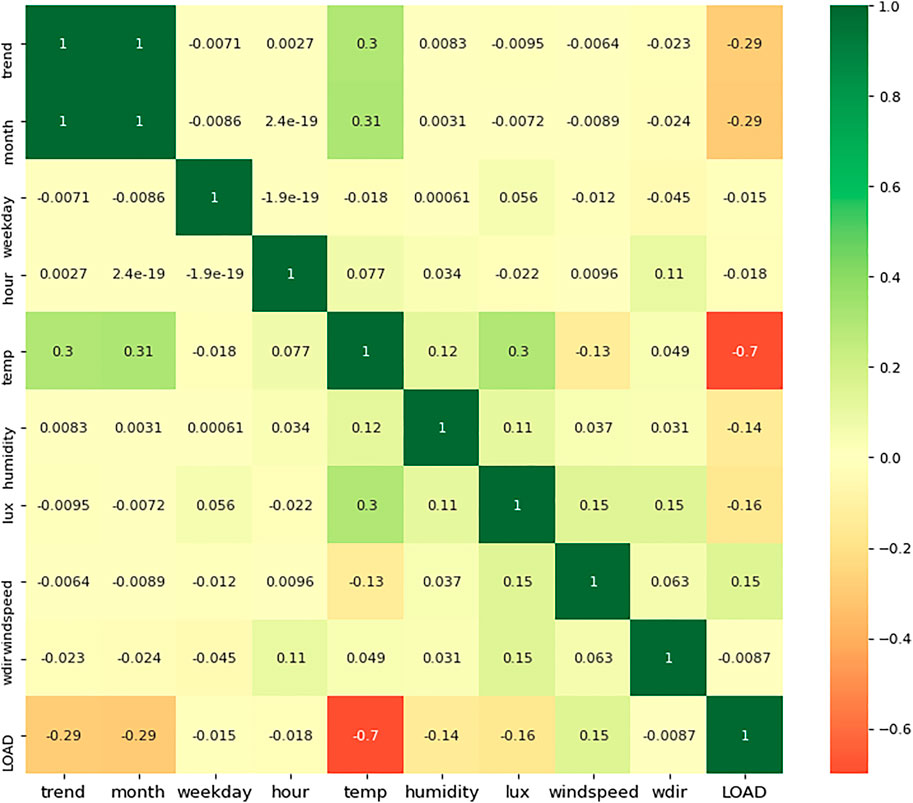
FIGURE 5. Correlation analysis between the available features.

TABLE 1

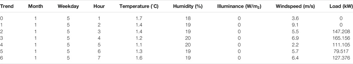
TABLE 1. Example of the database.

Result and Discussion

Model Parameter Setting

In this study, we used the Hyperopt framework to implement the TPE algorithm and automatically optimized the hyperparameters of all baseline models. The programming language is Python and the deep learning framework is TensorFlow2.0. Hyperopt is a Python library for hyperparametric optimization based on Bayesian optimization. It supports the optimization of continuous, discrete, and condition variables. Using the Hyperopt framework requires setting four parameters: specifying the objective function to be optimized, defining the search space with super parameters, Trails Database, and the search algorithm. This section will take the LSTM model as an example to outline the method of constructing the model. After the parameter optimization of the LSTM baseline model was completed, we added an attention layer after the hidden layer of the LSTM model to build the A-LSTM model.

The LSTM baseline model needs to optimize four parameters, which are the time step L of each layer in LSTM (using the length of the previous data), the size of the hidden unit m of each layer, the size of the batch processing b in the training process (we used the two-layer LSTM structure, and set the same hidden unit for each layer by default), and the drop rate of the Dropout layer. To determine the range of L, we first performed autocorrelation analysis on load data to identify data cycle patterns, and the results are shown in Figure 6. In Figure 6, the X-axis represents “hours” and the Y-axis represents the autocorrelation coefficient. We found that the overall autocorrelation of the load is in the form of cycle decline, and the autocorrelation of the load is a cycle of 24 h, which means the autocorrelation peak occurs every 24 h. Therefore, we define the conditional parameters of L as (12, 24, 36, 48). To avoid overfitting, we added a dropout layer after each LSTM layer, and the conditional parameters of drop rate are (0.2, 0.3, 0.4, 0.5). Due to the limited computational force, based on ensuring the prediction accuracy, we set the conditional parameter sets of m and b based on the empirical method: m ∈{32,64,128,256} and b ∈{32,64,128,256} (Wang et al., 2019b). We input the above conditional parameters into the Hyperopt framework and use the TPE algorithm to optimize the model’s super parameters. Figure 7 shows the optimized RNN, LSTM, and A-LSTM model structure, the hyperparameters of these models are determined by the TPE algorithm.

FIGURE 6

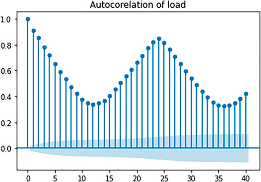
FIGURE 6. Load autocorrelation analysis results.

FIGURE 7

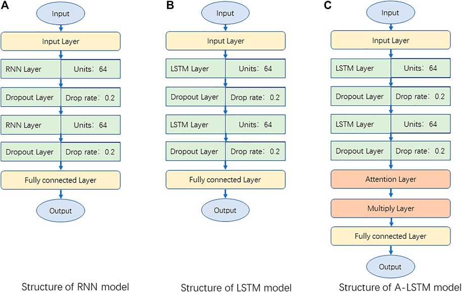
FIGURE 7. Structure of RNN, LSTM, and A-LSTM model.

Since the above three models are all recurrent neural networks, we also set up the DNN model and the SVR model for horizontal comparison. These two models also input all the data 24 h before the time slot t and the time data at the time slot t to predict and finally output the load data at the time slot t. The optimal hyperparameters of the DNN model optimized by the TPE algorithm are shown in Table 2. The optimal hyperparameters of the SVR model optimized by the TPE algorithm are shown in Table 3. The topology of the above five models depends on the characteristics of the KSRP dataset, so for the other datasets, the structure and hyperparameters of the model should be adjusted according to the data. Since the focus of this study was to explore the potential of the LSTM model with the attention mechanism in the field of load prediction. Therefore, on the premise of ensuring the prediction accuracy, the topological structure and input characteristics of the model were simplified as far as possible, to improve the generalization ability of the model and reduce the required computational force.

TABLE 2

TABLE 2. Hyperparameters for DNN model.

TABLE 3

TABLE 3. Hyperparamers for SVR model.

Annual Prediction Performance Comparison

To evaluate the time series prediction effect of the A-LSTM model on this data set, we compared it with the same type of RNN, LSTM model, and DNN model without memory function in this experiment. All models have been trained and tested 5 times, and the final data used for comparison is the average of the five test results to reduce the errors caused by random numbers. Root Mean Square Error (RMSE), Mean Absolute Error (MAE), and R-Square Value (R2_SCORE) were used as indicators of the evaluation model, which were calculated according to Eqs 15–17. The $y_i$ denotes the real observations, ${\overline{y}}_i$ denotes the average of the observed value, ${\tilde{y}}_i$ denotes the predicted value, N denotes the number of test samples.

$RMSE=\sqrt{\frac{1}{n}{\displaystyle \sum }_{i=1}^n{\left(y_i-{\tilde{y}}_i\right)}^2}(15)$

$MAE=\frac{1}{N}{\displaystyle \sum }_{i=1}^N\left|y_i-{\tilde{y}}_i\right|(16)$

$R^2=1-\frac{{\Sigma }_{\text{i}=1}^n{\left(y_i-\widetilde{y_i}\right)}^2}{{\Sigma }_{\text{i}=1}^n{\left(y_i-{\overline{y}}_i\right)}^2}(17)$

We first used the data of 8 years (from 2002 to 2009) as the training set to train the models and evaluated the effect of the load forecast in 2010. The results of the five models respectively predicting the annual data of 2010 are shown in Table 4. It could be seen that although the prediction results of each model were close to, the prediction accuracy of the A-LSTM model was the highest. Compared with the second-best predicted LSTM, A-LSTM’s RMSE decreased by 3.06%, MSE decreased by 6.54%, and R² value increased by 0.43%. The reason why the evaluation results are close is that the system operates under low or zero load for a large amount of time in a year, and the prediction error during these periods is very small, which may reduce the overall average prediction error. We will explore this phenomenon in the next section.

TABLE 4

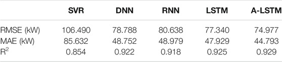
TABLE 4. Comparison of prediction errors between different models.

To explore the influence of the size of the training set on the prediction accuracy of the model, we also conducted the following experiments: keeping the topological structure of the above five models unchanged, gradually reducing the training set in a unit of 2 years, and the 2010 data were used as the test set to evaluate each model separately. The experimental results are shown in Figure 8. We found that the prediction accuracy of each model decreases with the reduction of the training set. The experiment shows that the prediction accuracy of the A-LSTM model was the best when the data of 8, 6, and 4 years were used as the training set. Compared with the suboptimal LSTM model, its RMSE decreased by 3.06, 10.86, and 11.29%, respectively. R² value increased by 0.43, 2.21, and 2.57%, respectively. However, when 2 years’ data were used as the training set, the prediction accuracy of the A-LSTM model decreased significantly, and its prediction accuracy was only better than that of the SVR model. This indicates that the prediction accuracy of the A-LSTM model will increase with the length of training set, and the prediction accuracy of 4-years or 6-years data sets of the A-LSTM model has obvious advantages compared with other models. This means that when the length of training set is greater than a certain threshold (6–8 years), the advantage of its prediction accuracy will gradually decrease compared with other cyclic neural network models. Besides, when the length of the training set is less than A certain threshold value (4–2 years), the prediction accuracy of the A-LSTM model will decrease significantly.

FIGURE 8

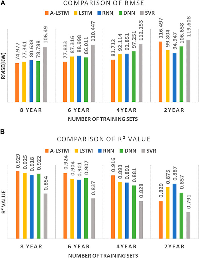
FIGURE 8. The prediction accuracy of each model under different lengths of training set: (A) the comparison of RMSE, (B) the comparison of R² value.

Prediction Performance Comparison at High and Low Loads

In the previous section, we discussed how a large number of zero-load and low-load forecasts over a year may affect the average error. To more intuitively evaluate the prediction effect of the A-LSTM model, we selected data of 2 weeks in each of four periods in the 2010 years for comparison. Among the data selected for the experiment, two groups were high-load period data (2010.1.1 to 2010.1.14 and 2010.8.1 to 2010.1.14), and the other two groups were low-load period data (2010.3.1 to 2010.3.14 and 2010.5.16 to 2010.5.30). the results are shown in Table 5. As can be seen from Table 4, the prediction accuracy of the A-LSTM model was significantly higher than that of other models. In the high heating load stage, compared with the second-best predicted LSTM, A-LSTM’s RMSE decreased by 10.02%, MSE decreased by 5.93%, and R² value increased by 2.59%; In the high cooling load stage, RMSE of A-LSTM decreased by 9.21%, MSE decreased by 8.80%, and R² value increased by 1.88%, compared with that of the second-best predicted LSTM. In the low heating load stage, compared with the second-best predicted LSTM, A-LSTM’s RMSE decreased by 6.25%, MSE decreased by 3.94%, and R² value increased by 5.14%; In the low cooling load stage, RMSE of A-LSTM decreased by 5.24%, MSE decreased by 4.47%, and R² value increased by 2.36%, compared with that of the second-best predicted RNN. This indicates that compared with the low-load stage, A-LSTM in the high-load stage has an obvious improvement compared with other models, which also indicates that A-LSTM has more potential in peak prediction. It can be seen from Table 5 that the prediction accuracy of the five models for the cooling load is higher than that for the heating load. Taking the A-LSTM model as an example, RMSE decreased by 18.515 (kW), MAE decreased by 15.733 (kW), and R² value increased by 0.051 in the peak cooling period compared with the peak heating period. This change was also evident during periods of low load.

TABLE 5

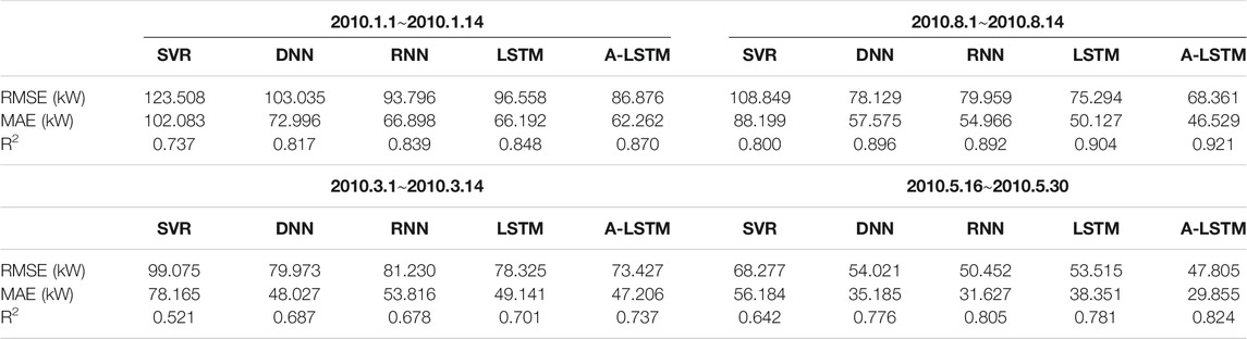
TABLE 5. Performance of A-LSTM models compared to the baseline model.

To explain this phenomenon, the characteristic correlation coefficients of the cooling season and heating season were statistically analyzed. Figure 9 can explain the reasons for the above phenomena from one perspective. It can be seen from Figure 9 that the correlation coefficients between the load and other characteristics in the refrigeration season are higher than those in the heating season, especially the temperature, illumination, and humidity. This indicates that the output of cooling load is more affected by environmental factors, while the output of heat load is more affected by the laws of human production and life. The existing data cannot fully reflect the laws of human production and life, but it reflects the environmental factors more comprehensively, so this phenomenon occurs.

FIGURE 9

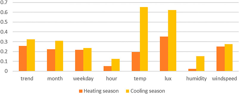
FIGURE 9. Absolute value of correlation coefficients of load and other features in the database between heating season and cooling season.

The actual prediction curves corresponding to Table 5 are shown in Figure 10. As can be seen from the fitting curve results, the load output of the KSRP system in the high load stage was distributed discretely, and it fluctuated greatly in the short term, as the peaks and troughs often appear alternately in the time series. Except for the SVR model, other models had a good fitting effect. By comparing R² values in Table 5, we also found that the prediction curve fitting rate of all models, including the A-LSTM model, was higher in the high load period than in the low load period. It could also be seen from Figure 10 that the curve fitting effect in the period of the high load was better than that in the period of low load. This indicates that the load in the low load stage is more affected by random factors and is more difficult to predict.

FIGURE 10

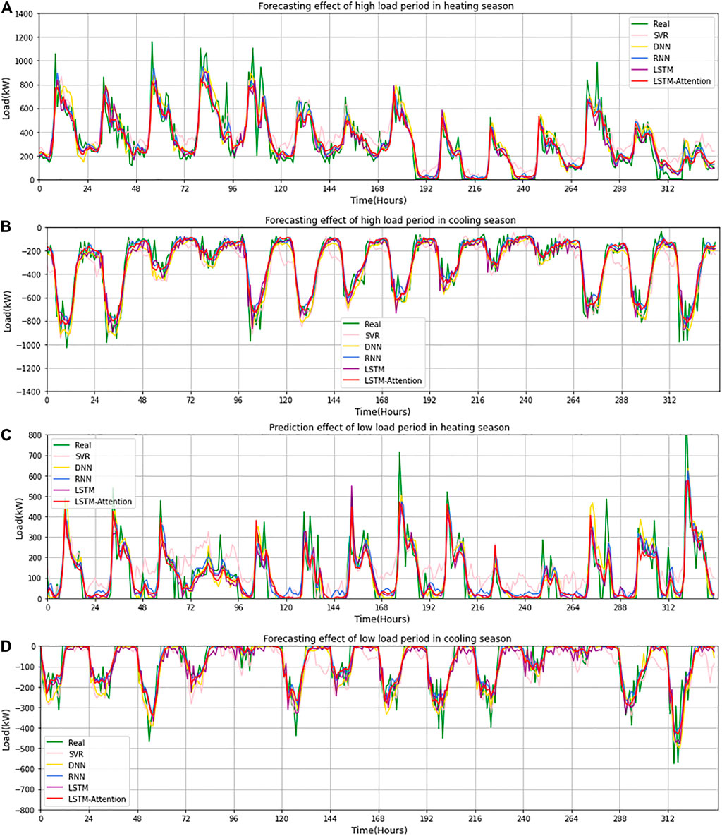
FIGURE 10. Predicted load use versus measured load use by different models for 2 weeks as a test period: (A) Forecasting effect of high load period in the heating season, (B) Forecasting effect of high load period in the cooling season, (C) Forecasting effect of low load period in the heating season, (D) Forecasting effect of low load period in the cooling season.

There are two limitations in the current study. First, due to the limited computational force, the search method adopted in the hyperparameter optimization in this paper is based on the conditional parameters, rather than the search based on the assignment interval. Although the conditional parameters based on the empirical method can ensure the accuracy of the prediction, it is undeniable that there is room for further optimization of the super parameters of the models. Secondly, the Bahdanau algorithm adopted is the classical gradient-based method to obtain the optimal solution. The gradient-based method has the advantage of easy implementation, but at the same time, it will bring premature convergence and the problem of falling into a locally optimal solution. Therefore, there is room for further optimization at the algorithm level of this study.

Conclusion

Predictive control had attracted more and more attention in building energy efficiency. Previous studies had shown that the HVAC system of large buildings was complex in structure, and its operation was affected by random environmental factors and human activities, so it was very challenging to predict its short-term HVAC load. In this paper, we first analyzed the underlying patterns in the data based on the actual operation data of KSRP Energy Center in 9 years and then determined the factors used to establish the model according to the results of the Pearce correlation calculation. The results showed that the cooling and heating load of HVAC was most affected by the outdoor temperature, and the time of daily peak load was concentrated in a specific period.

Therefore, this paper proposed a new model combining the attention mechanism with the LSTM neural network, which was implemented by the following steps: First, according to the autocorrelation analysis results of HVAC load, we determined the data of the previous 24 h as the time step to predict the load of the next hour. In the second step, we used the TPE optimization method to optimize the hyperparameters of the baseline LSTM model. The test results showed that the LSTM model with two layers of 64 neurons had the best prediction effect. Thirdly, we added the attention layer to the baseline LSTM model to build the A-LSTM model. Finally, we also set up RNN, DNN, and SVR models as horizontal comparison objects.

Finally, we took the data from KSRP Energy Center from 2002 to 2009 as the training set and the data from 2010 as the test set to test the above five models respectively. The results showed that the prediction accuracy of the A-LSTM model was the best. Compared with the LSTM model, the overall RMSE decreased by 3.06%, MSE decreased by 6.54%, and R² value increased by 0.43%. By progressively reducing the size of the training set, we found that the performance advantage of the A-LSTM model was most significant when the length of training set was between 4 and 6 years. Besides, when the size of the training set dropped to 2 years, the prediction accuracy of the A-LSTM model declined sharply, which indicates that it has limitations in predicting small sample data. To verify the impact of low-load and zero-load samples on the experimental results, we respectively selected four typical operating mode samples in 2010 for evaluation and drew the effect chart of the predicted results. The results showed that the prediction effect of the A-LSTM model for refrigeration load was better than that for heating load, and the prediction effect for the high load period is better than that for the low load period.

In conclusion, for the cooling and heating load prediction of large buildings, the introduction of the attention mechanism can not only effectively improve the prediction accuracy of the traditional LSTM model, but also improve the accuracy of peak prediction. However, in practical application, the prediction effect of this model for different operating modes is different, which in-depth influence mechanism and solutions need to be further analyzed. Besides, there is still room for optimization in the algorithm of attention mechanism. In future work, we will try to apply the A-LSTM model to real-time HVAC energy-saving control. Since the traditional MPC system is a model-based control system, it needs to model the controlled objects accurately, which may affect the generality of the model. Therefore, we are more inclined to adopt a model-free deep reinforcement learning (RL) algorithm to solve this problem, such as taking the predicted value as the observed state of the agent to improve the control accuracy of the RL model.

Data Availability Statement

The raw data supporting the conclusions of this article will be made available by the authors, without undue reservation.

Author Contributions

WG, FQ, and YL contributed to the conception and design of the study. YX organized the database. YX performed the statistical analysis. YX wrote the first draft of the manuscript. WG, FQ, and YL wrote sections of the manuscript. All authors contributed to manuscript revision, read, and approved the submitted version.

Conflict of Interest

The authors declare that the research was conducted in the absence of any commercial or financial relationships that could be construed as a potential conflict of interest.

Publisher’s Note

All claims expressed in this article are solely those of the authors and do not necessarily represent those of their affiliated organizations, or those of the publisher, the editors and the reviewers. Any product that may be evaluated in this article, or claim that may be made by its manufacturer, is not guaranteed or endorsed by the publisher.

References

Askari, S., Montazerin, N., and Zarandi, M. H. F. (2015). A Clustering Based Forecasting Algorithm for Multivariable Fuzzy Time Series Using Linear Combinations of Independent Variables[J]. Appl. Soft Comput. 35, 151–160.

CrossRef Full Text | Google Scholar

Bahdanau, D., Cho, K., and Bengio, Y. (2014). Neural Machine Translation by Jointly Learning to Align and Translate[J]. arXiv.

Bui, D-K., Nguyen, T. N., Ngo, T. D., and Nguyen-Xuan, H. (2020). An Artificial Neural Network (ANN) Expert System Enhanced with the Electromagnetism-Based Firefly Algorithm (EFA) for Predicting the Energy Consumption in Buildings[J]. Energy 190, 116370.

CrossRef Full Text | Google Scholar

Chang, F., Chen, T., Su, W., and Alsafasfeh, Q. (2020). Control of Battery Charging Based on Reinforcement Learning and Long Short-Term Memory Networks[J]. Comput. Electr. Eng. 85, 106670.

CrossRef Full Text | Google Scholar

Deb, C., Eang, L. S., Yang, J., and Santamouris, M. (2016). Forecasting Diurnal Cooling Energy Load for Institutional Buildings Using Artificial Neural Networks[J]. Energy and Buildings 121, 284–297.

CrossRef Full Text | Google Scholar

Guo, Z., Zhou, K., Zhang, X., and Yang, S. (2018). A Deep Learning Model for Short-Term Power Load and Probability Density Forecasting[J]. Energy 160, 1186–1200.

CrossRef Full Text | Google Scholar

Hazyuk, I., Ghiaus, C., and Penhouet, D. (2012). Optimal Temperature Control of Intermittently Heated Buildings Using Model Predictive Control: Part II – Control Algorithm[J]. Building Environ. 51, 388–394.

CrossRef Full Text | Google Scholar

Heidari, A., and Khovalyg, D. (2020). Short-term Energy Use Prediction of Solar-Assisted Water Heating System: Application Case of Combined Attention-Based LSTM and Time-Series Decomposition[J]. Solar Energy 207, 626–639.

CrossRef Full Text | Google Scholar

Hochreiter, S., and Schmidhuber, J. (1997). Long Short-Term Memory[J]. Neural Comput. 9 (8), 1735–1780.

PubMed Abstract | CrossRef Full Text | Google Scholar

Huang, G., and Chow, T-T. (2011). Uncertainty Shift in Robust Predictive Control Design for Application in CAV Air-Conditioning Systems[J]. Building Serv. Eng. Res. Tech. 32 (4), 329–343.

CrossRef Full Text | Google Scholar

Iqbal, W., Tang, Y. M., Chau, K. Y., Irfan, M., and Mohsin, M. (2021). Nexus between Air Pollution and NCOV-2019 in China: Application of Negative Binomial Regression Analysis[J]. Process Saf. Environ. Prot. 150, 557–565.

CrossRef Full Text | Google Scholar

Jradi, M., Veje, C., and Jørgensen, B. N. (2017). Deep Energy Renovation of the Mærsk Office Building in Denmark Using a Holistic Design Approach[J]. Energy and Buildings 151, 306–319.

CrossRef Full Text | Google Scholar

Kim, B., Yamaguchi, Y., Kimura, S., Ko, Y., Ikeda, K., and Shimoda, Y. (2019). Urban Building Energy Modeling Considering the Heterogeneity of HVAC System Stock: A Case Study on Japanese Office Building Stock[J]. Energy and Buildings 199, 547–561.

CrossRef Full Text | Google Scholar

Li, J., Wang, F., and He, Y. (2020). Electric Vehicle Routing Problem with Battery Swapping Considering Energy Consumption and Carbon Emissions[J]. Sustainability 12 (24).

CrossRef Full Text | Google Scholar

Li, J., Yang, B., Li, H., Wang, Y., Qi, C., and Liu, Y. (2021A), DTDR–ALSTM: Extracting Dynamic Time-Delays to Reconstruct Multivariate Data for Improving Attention-Based LSTM Industrial Time Series Prediction Models[J], Knowledge-Based Systems, 211, 106508. doi:10.1016/j.knosys.2020.106508

CrossRef Full Text | Google Scholar

Li, R., Xu, M., Chen, Z., Gao, B., Cai, J., Shen, F., et al. (2021B). Phenology-based Classification of Crop Species and Rotation Types Using Fused MODIS and Landsat Data: The Comparison of a random-forest-based Model and a Decision-Rule-Based Model[J]. Soil Tillage Res. 206, 104838.

CrossRef Full Text | Google Scholar

Li, W., Chien, F., Hsu, C-C., Zhang, Y., Nawaz, M. A., Iqbal, S., et al. (2021C). Nexus between Energy Poverty and Energy Efficiency: Estimating the Long-Run Dynamics[J]. Resour. Pol. 72, 102063.

CrossRef Full Text | Google Scholar

Li, Y., Zhu, Z., Kong, D., Han, H., and Zhao, Y. (2019). EA-LSTM: Evolutionary Attention-Based LSTM for Time Series Prediction[J]. Knowledge-Based Syst. 181 (Oct.1), 1047851–1047858.

CrossRef Full Text | Google Scholar

Liang, Y., Ke, S., Zhang, J., Yi, X., and Zheng, Y. (2018), GeoMAN: Multi-Level Attention Networks for Geo-Sensory Time Series Prediction[C], Proceedings of the Twenty-Seventh International Joint Conference on Artificial Intelligence IJCAI-18.Stockholm, Sweden, July 13-19, 2018.

Google Scholar

Liu, M-D., Ding, L., and Bai, Y-L. (2021). Application of Hybrid Model Based on Empirical Mode Decomposition, Novel Recurrent Neural Networks and the ARIMA to Wind Speed Prediction[J]. Energ. Convers. Manag. 233, 113917.

CrossRef Full Text | Google Scholar

Lu, J., Xiong, C., Parikh, D., and Socher, R. (2017). Knowing when to Look: Adaptive Attention via A Visual Sentinel for Image Captioning[C], Proceedings of the 2017 IEEE Conference on Computer Vision and Pattern Recognition (CVPR). Honolulu, HI, USA, 21-26 July 2017, doi:10.1109/CVPR.2017.345

CrossRef Full Text | Google Scholar

Luo, H., Cai, J., Zhang, K., Xie, R., and Zheng, L. (2021). A Multi-Task Deep Learning Model for Short-Term Taxi Demand Forecasting Considering Spatiotemporal Dependences[J]. J. Traffic Transportation Eng. (English Edition) 8 (1), 83–94.

CrossRef Full Text | Google Scholar

Lv, Z., Qiao, L., Li, J., and Song, H. (2021). Deep-Learning-Enabled Security Issues in the Internet of Things[J]. IEEE Internet Things J. 8 (12), 9531–9538.

CrossRef Full Text | Google Scholar

Lv, Z., Qiao, L., Singh, A. K., and Wang, Q. (2021). Fine-grained Visual Computing Based on Deep Learning[J]. ACM Transactions on Multimidia Computing Communications and Applications, 17. doi:10.1145/3418215

CrossRef Full Text | Google Scholar

Lv, Z., Singh, A., and Li, J. (2021). Deep Learning for Security Problems in 5G Heterogeneous Networks[J]. IEEE Netw. 35, 67–73.

CrossRef Full Text | Google Scholar

Ma, W., Fang, S., Liu, G., and Zhou, R. (2017). Modeling of District Load Forecasting for Distributed Energy System[J]. Appl. Energ. 204, 181–205.

CrossRef Full Text | Google Scholar

Ma, Z., Ye, C., Li, H., and Ma, W. (2018). Applying Support Vector Machines to Predict Building Energy Consumption in China[J]. Clean. Energ. Clean. Cities 152, 780–786.

CrossRef Full Text | Google Scholar

Massana, J., Pous, C., Burgas, L., Melendez, J., and Colomer, J. (2015). Short-term Load Forecasting in a Non-residential Building Contrasting Models and Attributes[J]. Energy and Buildings 92, 322–330.

CrossRef Full Text | Google Scholar

Mayne, D. Q. (2014). Model Predictive Control: Recent Developments and Future Promise[J]. Automatica 50 (12), 2967–2986.

CrossRef Full Text | Google Scholar

Mohsin, M., Hanif, I., Taghizadeh-Hesary, F., Abbas, Q., and Iqbal, W. (2021). Nexus between Energy Efficiency and Electricity Reforms: A DEA-Based Way Forward for Clean Power Development[J]. Energy Policy 149, 112052.

CrossRef Full Text | Google Scholar

Mohsin, M., Taghizadeh-Hesary, F., Panthamit, N., Anwar, S., Abbas, Q., and Vo, X. V. (2020). Developing Low Carbon Finance Index: Evidence from Developed and Developing Economies[J]. Finance Res. Lett., 101520.

CrossRef Full Text | Google Scholar

Nguyen, H-P., Liu, J., and Zio, E. (2020). A Long-Term Prediction Approach Based on Long Short-Term Memory Neural Networks with Automatic Parameter Optimization by Tree-Structured Parzen Estimator and Applied to Time-Series Data of NPP Steam Generators[J]. Appl. Soft Comput. 89, 106116.

CrossRef Full Text | Google Scholar

Qian, F., Gao, W., Yang, Y., and Yu, D. (2020). Potential Analysis of the Transfer Learning Model in Short and Medium-Term Forecasting of Building HVAC Energy Consumption[J]. Energy 193, 116724.

CrossRef Full Text | Google Scholar

Sendra-Arranz, R., and Gutiérrez, A. (2020). A Long Short-Term Memory Artificial Neural Network to Predict Daily HVAC Consumption in Buildings[J]. Energy and Buildings 216, 109952.

CrossRef Full Text | Google Scholar

Su, C., Huang, H., Shi, S., Jian, P., and Shi, X. (2020). Neural Machine Translation with Gumbel Tree-LSTM Based Encoder[J]. J. Vis. Commun. Image Representation 71, 102811.

CrossRef Full Text | Google Scholar

Sultana, W. R., Sahoo, S. K., Sukchai, S., Yamuna, S., and Venkatesh, D. (2017). A Review on State of Art Development of Model Predictive Control for Renewable Energy Applications[J]. Renew. Sust. Energ. Rev. 76, 391–406.

CrossRef Full Text | Google Scholar

Sun, H., Awan, R. U., Nawaz, M. A., Mohsin, M., Rasheed, A. K., and Iqbal, N. (2021). Assessing the Socio-Economic Viability of Solar Commercialization and Electrification in South Asian Countries, Environment, Dev. Sustainability, 23, 9875–9897.

CrossRef Full Text | Google Scholar

Verwimp, L., Van Hamme, H., and Wambacq, P. (2020). State Gradients for Analyzing Memory in LSTM Language Models[J]. Comp. Speech Lang. 61, 101034.

CrossRef Full Text | Google Scholar

Wang, J., Huang, G., Sun, Y., and Liu, X. (2016). Event-driven Optimization of Complex HVAC Systems[J]. Energy and Buildings 133, 79–87.

CrossRef Full Text | Google Scholar

Wang, W., Hong, T., Xu, X., Chen, J., Liu, Z., and Xu, N. (2019). Forecasting District-Scale Energy Dynamics through Integrating Building Network and Long Short-Term Memory Learning Algorithm[J]. Appl. Energ. 248, 217–230.

CrossRef Full Text | Google Scholar

Wang, Z., Hong, T., and Piette, M. A. (2020). Building thermal Load Prediction through Shallow Machine Learning and Deep Learning[J]. Appl. Energ. 263, 114683.

CrossRef Full Text | Google Scholar

Wang, Z., Hong, T., and Piette, M. A. (2019). Predicting Plug Loads with Occupant Count Data through a Deep Learning Approach[J]. Energy 181, 29–42.

CrossRef Full Text | Google Scholar

Wang, Z., Liu, J., Zhang, Y., Yuan, H., Zhang, R., and Srinivasan, R. S. (2021). Practical Issues in Implementing Machine-Learning Models for Building Energy Efficiency: Moving beyond Obstacles[J]. Renew. Sust. Energ. Rev. 143, 110929.

CrossRef Full Text | Google Scholar

Wei, Y., Xia, L., Pan, S., Wu, J., Zhang, X., Han, M., et al. (2019). Prediction of Occupancy Level and Energy Consumption in Office Building Using Blind System Identification and Neural Networks[J]. Appl. Energ. 240, 276–294.

CrossRef Full Text | Google Scholar

Yang, F., Wang, D., Xu, F., Huang, Z., and Tsui, K-L. (2020). Lifespan Prediction of Lithium-Ion Batteries Based on Various Extracted Features and Gradient Boosting Regression Tree Model[J]. J. Power Sourc. 476, 228654.

CrossRef Full Text | Google Scholar

Yang, J. J., Yang, M., Wang, M. X., Du, P. J., and Yu, Y. X. (2020). A Deep Reinforcement Learning Method for Managing Wind Farm Uncertainties through Energy Storage System Control and External reserve Purchasing[J]. Int. J. Electr. Power Energ. Syst. 119, 105928.

CrossRef Full Text | Google Scholar

Yang, T., Li, B., and Xun, Q. (2019), LSTM-Attention-Embedding Model-Based Day-Ahead Prediction of Photovoltaic Power Output Us-Ing Bayesian Optimization[J]. IEEE Access, 7, 171471-171484, 1-1.PP(99, doi:10.1109/ACCESS.2019.2954290

CrossRef Full Text | Google Scholar

Yu, B. (2021). Urban Spatial Structure and Total-Factor Energy Efficiency in Chinese Provinces[J]. Ecol. Indicators 126, 107662.

CrossRef Full Text | Google Scholar

Yu, Z., Yu, J., Fan, J., and Tao, D. (2017), Multi-modal Factorized Bilinear Pooling with Co-attention Learning for Visual Question Answering[C], 2017 IEEE International Conference on Computer Vision (ICCV), Venice, Italy, 22-29 Oct. 2017, doi:10.1109/ICCV.2017.202

CrossRef Full Text | Google Scholar

Zhan, S., and Chong, A. (2021). Data Requirements and Performance Evaluation of Model Predictive Control in Buildings: A Modeling Perspective[J]. Renew. Sust. Energ. Rev. 142, 110835.

CrossRef Full Text | Google Scholar

Zhao, X., Gao, W., Qian, F., and Ge, J. (2021). Electricity Cost Comparison of Dynamic Pricing Model Based on Load Forecasting in home Energy Management System[J]. Energy 229, 120538.

CrossRef Full Text | Google Scholar