- 1State Grid Liaoning Electric Power Co., Ltd., Shenyang, China
- 2State Grid Shenyang Power Supply Company, Shenyang, China
- 3School of Electrical Engineering, Northeast Electric Power University, Jilin, China
Compared to the step tariff, the real-time pricing (RTP) could be more stimulated for household consumers to change their electricity consumption behaviors. It can reduce the reserve capacity, peak load, and of course the electricity bill, which could achieve the purpose of saving energy. This paper proposes a coordinated optimization algorithm and data-driven RTP strategy in electricity market. First, the electricity price is divided into two parts, basic electricity price and fluctuating price. When the electricity consumption is equal to the average daily electricity consumption, the price is defined as the basic electricity price, which is the clearing electricity price. The consumer electricity data are analyzed. A random forest algorithm is adopted to predict the load data. Optimal adjustment parameters are obtained and the load fluctuation and the fluctuation of the electricity price are further quantified. Secondly, the appliances are modeled. The operation priority is established based on the preferences of customers and the Monte Carlo method is used to form the power load curve. Then, the smart energy planning unit is proposed to optimize the appliances on/off time and running time of residential electrical appliances. An incentive mechanism is used to further standardize the temporary electricity consumption. An improved multiobjective particle swarm optimization (IMOPSO) algorithm is adopted, which adopts the linear weighted evaluation function method to maximize the consumer’s social welfare while minimizing the electricity bill. The simulation proves that the stability of the power grid is improved while obtaining the best power strategy.
Introduction
Power consumers have coincident peak load, resulting in a large peak-valley difference. For traditional power supplies, the spare capacity is relatively large, which increases the operating cost of the system. In order to reduce the peak-valley difference and enhance the stability of power supply, optimization methods were proposed from the power generation side and the load side, such as time-of-use electricity price (TOU) and Demand Response (DR). The demand side self-adjustment is more economical and practical than the investment in the power side to meet the peak demand (Li et al., 2021). To establish a standardized and healthy electricity market, it is necessary to give full play to the leverage of electricity prices in the electricity market. In recent years, TOU has played an increasingly important role in the power industry of various countries in the world and has also attracted widespread attention in the academic field (Lampropoulos et al., 2012). After the implementation of the TOU, the load demand is increased during the low period and the load demand is reduced during the peak period, in which way the consumer has an economical benefit (i.e., low utility bill). So it can change the electricity consumption behavior of consumers. Currently, the pricing models mainly include tiered electricity price (TP), real-time pricing (RTP), day-ahead pricing (DAP), time-of-use pricing (TOUP), and critical peak pricing (CPP). Zhou B. proposed a new multiobjective optimal electricity price setting model for time-of-use electricity price and stepped electricity price, which can save energy and transfer the load from peak hours to off-peak hours (Zhou et al., 2018). Mohsenian-Rad A. H. considered deployment of energy consumption scheduling (ECS) equipment in smart meters to implement autonomous demand side management in communities where multiple buildings share energy (Mohsenian-Rad et al., 2010). This article mainly studies a source of energy (a generator or step-down substation transformer) connected to the grid, without considering regional interconnection issues. From the long-term implementation of the time-of-use electricity price experience, it is found that the range of the peak-to-valley price ratio is usually between two and five times (Li et al., 2015). Based on the game theory method, a pricing model is proposed to reduce the total energy consumption cost and the peak-to-average load ratio (PAR). The use of a smart residential energy management system (SREMS) is demonstrated at the consumers’ premises to reduce the total electricity bill by optimally time scheduling the operation of household appliances. Related topics of home smart power consumption management unit are being widely studied. A new intelligent management system to accommodate the possible optimal decisions for elastic load consumption is discussed in an informational rich smart electricity grid (Alamaniotis (2020). How much of the elastic load for that specific day has been already scheduled? The temporary power demand of consumer is not considered in this paper. An increase in distributed small-scale generation and storage in residential prosumer households, Heinisch et al. (2019). The paper aims at investigating how residential photovoltaic (PV)-battery systems are operated in given different assumed incentives. However, this paper does not propose how to coordinate the battery charging and discharging strategies in the system case and household cost optimization.
This article first proposes a new RTP. The final electricity price consists of clearing price and fluctuating price. The relationship between load power consumption fluctuation and fluctuating electricity price is quantified based on a stochastic forest algorithm. In the second part, a mathematical model of household electrical equipment is established. A smart energy planning unit is proposed to optimize the on/off time and running time of residential electrical appliances. According to the equipment operation priority set by the consumers, a load forecasting model is proposed, and the Monte Carlo method is used to form a load curve. On this basis, incentive mechanisms are used to further regulate temporary electricity consumption. In the third part, the improved multiobjective particle swarm optimization (IMPSO) algorithm is used to optimize the calculation, so as to maximize the social welfare of consumers and minimize the cost of electricity. The optimal power consumption strategy is obtained, which also improves the stability of power grid. The simulation results show that the model reduces the consumers’ electricity bill, reduces the peak-valley difference of the system, and improves the stability of the system.
Establishment of Electricity Pricing Model
Load Forecasting Model Based on Stochastic Forest Algorithm
The establishment of electricity price mechanism is based on the stability of power grid. Consumers have a certain regularity in the behaviors of electricity consumption. The power consumption of four seasons in a year varies greatly. The power consumption in summer has increased significantly. If necessary, the energy must be limited to ensure the reliability of the power supply. Weather changes also affect the electricity consumption of consumers. The temperature rises, the cooling power increases significantly, and the electricity consumption fluctuates in rainy days. Therefore, load forecasting is related to weather factors, such as temperature and precipitation. Different weather factors affect the load in different ways. In the same season, weather factors affect the load in different ways. Therefore, the load data are classified by two indicators of weather temperature and rainfall.
The actual temperature at 8:00, 11:00, 12:00, 17:00, 18:00, 20:00
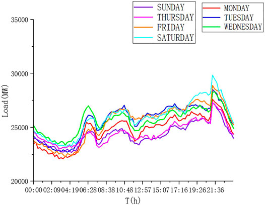
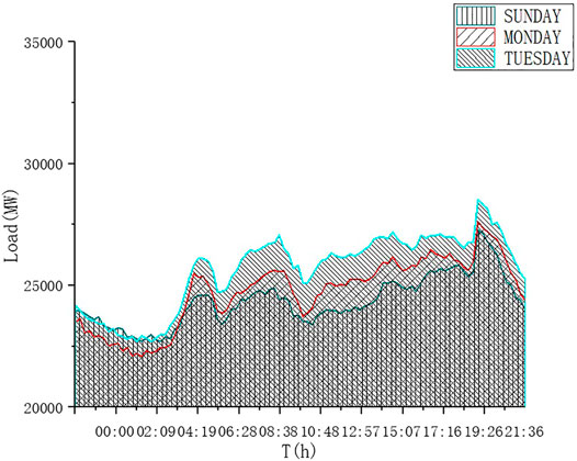
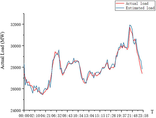
In random forest algorithm, each tree selects some samples and some features to avoid overfitting to a certain extent. Each tree randomly selects samples and randomly selects features, so that it has good antinoise ability and stable performance. It can handle very high-dimensional data and does not need to make feature selection. The decision trees of the random forest algorithm are independent of each other, the calculation speed is not affected and the training model is fast. The accuracy of the training results is high. The Monte Carlo method is used to generate the residential electricity consumption curve, which is more accurate and reliable than the historical simulation method. It also has a small amount of calculation. The traditional empirical method cannot approximate the real physical process, and it is difficult to obtain satisfactory results, while the Monte Carlo method can truly simulate the actual physical process, so the problem solving is very consistent with the reality, and very satisfactory results can be obtained. From Figure 1, it can be seen that the trend of electricity consumption in a week is basically the same, and the difference between peak and valley in a single day is about 30%. Mohsenian-Rad A H reckons that an efficient prediction is likely by looking at the prices on yesterday, the day before yesterday, and the same day last week. But the actual Monday load forecast accuracy is greatly affected by the previous day. From Figure 2, the electricity consumption pattern is quite different on weekends than on weekdays. As the load electricity consumption curve presents a certain regularity according to the week, the week is divided into seven groups, the load database is established, and the historical data are used to predict the power consumption of a certain day in the future. The Pauta criterion (3σ criterion) is selected to process the data. If the residual error is greater than 3σ, the data are considered abnormal and discarded. The standard deviation is usually used to replace the deviation (Qian, 2002).
It can be seen from the above that the weekly load data are divided into seven groups
where
Firstly, using the similar daily data, it is divided into two parts:
The forecast error rate
where
Establishment of Price Fluctuation Model
The equal area method is used to analyze the load forecasting curve and the average load value of the next day is obtain as
The electricity price consists of two parts, basic electricity price and electricity fluctuating price. The basic electricity price
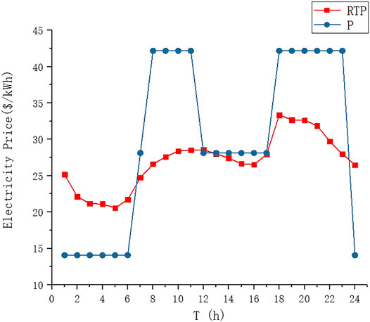
In order to avoid the unnecessary frequent fluctuation of electricity price, we ignore the situation that the fluctuation of electricity price is less than 5%. In the concept of IBR pricing, the marginal price increases with the total consumption (Reiss and White, 2005). Beyond the specific threshold of the total residential load per unit time, the electricity price will increase to a higher value. In Figure 4, it can be seen that TOU electricity price changes frequently. Compared with the step tariff, the change can highlight the regulation effect on hourly electricity consumption. The electricity price is relatively low in the early morning and at night, and the electricity price rises significantly in the morning and evening and the ladder rate changes largely. The larger price difference is conducive to the transfer of peak load, but it also makes it difficult for consumers to control the power consumption time. Therefore, it is necessary to use intelligent energy planning unit to manage the opening and closing time of household appliances.
Electric Application Model
After receiving the TOU price, the smart energy planning unit performs energy management planning. It selects a reasonable power consumption time based on consumers’ demand and plans the time length
where the consumer's application is
It can be seen from (5) that once the uninterruptible load starts to run, it will run uninterrupted until the task is completed to avoid any energy loss.
For electrical appliances with temperature restrictions, ensure that the temperature is within a reasonable range. For the cooling type operating coefficient
The Smart Energy Planning Unit
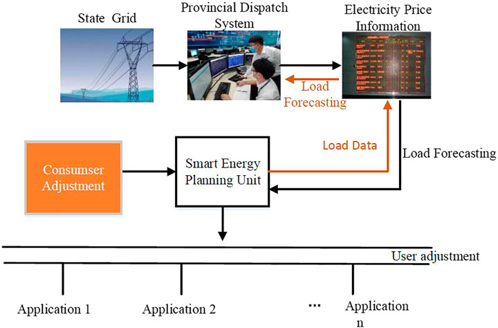
As shown in Figure 5, the smart energy planning unit obtains electricity price information through the local area network and sends instructions and receives messages through the home area network (HAN) (Hu, 2020). The information interaction network realizes the information interaction between smart modules and household appliances. The unit can capture the consumers’ electricity consumption rules and upload the forecast value of the next day's electricity demand to the grid through the regional network in advance. A two-way information transmission channel is formed, contributing to the company's power generation planning.
The Objective Function and Constraints
Goal 1. Optimize the electricity price model within the preset agreed conditions. The optimal electricity usage plan of the electricity customer within the day is obtained so that the electricity bill value generated on the day is the smallest. The optimization function of the electricity price model is
Due to the uncertainty of customer electricity usage rules. To ensure the reliability of power supply, it is necessary to establish an incentive mechanism for customers' energy management. For customers who continuously implement the electricity consumption plan for consecutive m days, the preferential state variable
Goal 2. Due to the particularity of electric energy, the total social welfare should be maximized while ensuring the minimum electricity bill for consumers. The implementation of real-time electricity prices will inevitably have a profound impact on consumers' electricity consumption behavior and the safe operation and management of the power grid. The social welfare maximization model is a model established from the perspective of the whole society as a whole, which fully reflects the interests of both supply and demand. The optimization problem is based on the basic model of the real-time electricity price pricing strategy that the government determines the electricity price or determines the guide price. The electricity price under the social welfare model will not exceed the fluctuation range required by the government to protect people's livelihood.
where
where
Constraints are shown in (5B)-(7).
When social welfare and electricity bill reach the optimal solution, respectively, their corresponding electricity consumption planning curves are different, which cannot make them reach the maximum value at the same time. Therefore, the multiobjective function is solved by linear weighted evaluation function method.
The multiobjective function obtained by linear weighting is expressed as
where
where
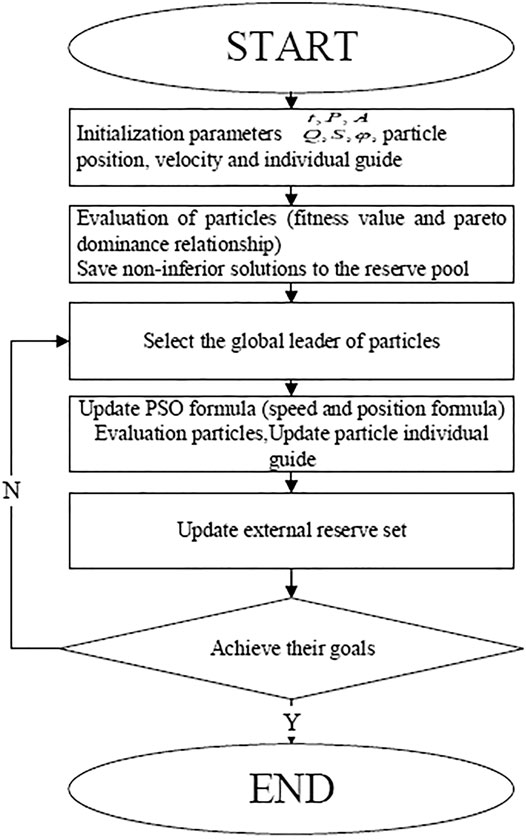
In this paper, the multiobjective particle swarm optimization algorithm is adopted to optimization. The calculation steps are shown in Figure 6.
Examples and Results
In this paper, the provincial load data of a certain area in Northeast China for the past three years are used to learn. The primary industry in this region currently accounts for 1.8% of the society, and the secondary industry is about 71.8% of the electricity consumption in the Northeast power grid. This shows that the northeast region has a relatively high degree of industrialization. The electricity consumption of the tertiary industry in Northeast China is about 14.5%. The part of urban and rural residents is about 11.9%. With the improvement of living standards, electricity consumption is still increasing. The electricity price data of PJM Dayton in 2019 are as the reference value of clearing electricity price to obtain the actual electricity price. In this paper, the Monte Carlo method is used to generate residential electricity consumption curve. About the parameter setting of electric application, the lower limit of the set temperature is 22°C, and the upper limit is 27°C. The optimum temperature is 25°C, and the scheduling period is
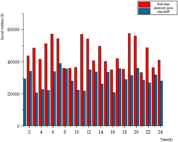
Assume that the number of consumers' appliances changes within 2–13, which are divided into fixed on-off equipment including lighting (p = 0.05 kWh) and induction cooker (about 1 kWh). Flexible control equipment includes humidifier (p = 0.05 kWh), oven (P = 1 kWh), and water dispenser (p = 0.6 kWh). From Figure 7, it can be seen that the real-time electricity price system has a certain effect on shifting the peak electricity load, and the peak electricity consumption of single-user residents has reduced about 40.13%.
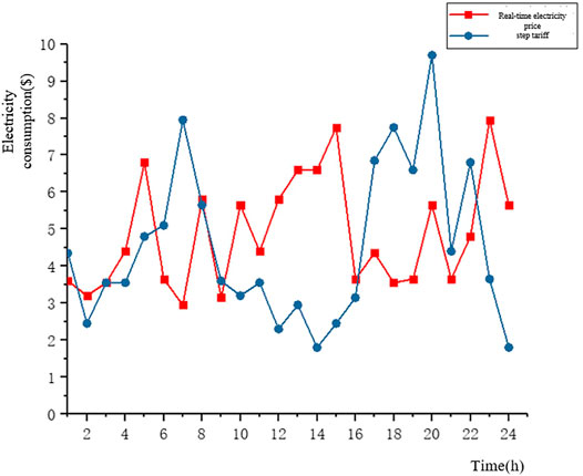
FIGURE 7. Comparison of daily electricity consumption between consumers’ real-time electricity price and step tariff.
To compare the impact of real-time electricity prices on consumers' electricity consumption behaviors and the impact on electricity bills, the following two scenarios are set up.
Scene 1. Consider only the perspective of consumers, without considering the social welfare. The consumers’ comfort index is proposed to quantify the consumers’ comfort level as Eq. 16, which reflects user satisfaction with electricity.
Scene 2. On the premise of ensuring social welfare, consider the economics and comfort of electricity customers.
Eq. 8 is optimized by particle swarm algorithm (Venter and Jaroslaw, 2003), and the upper limit of
where
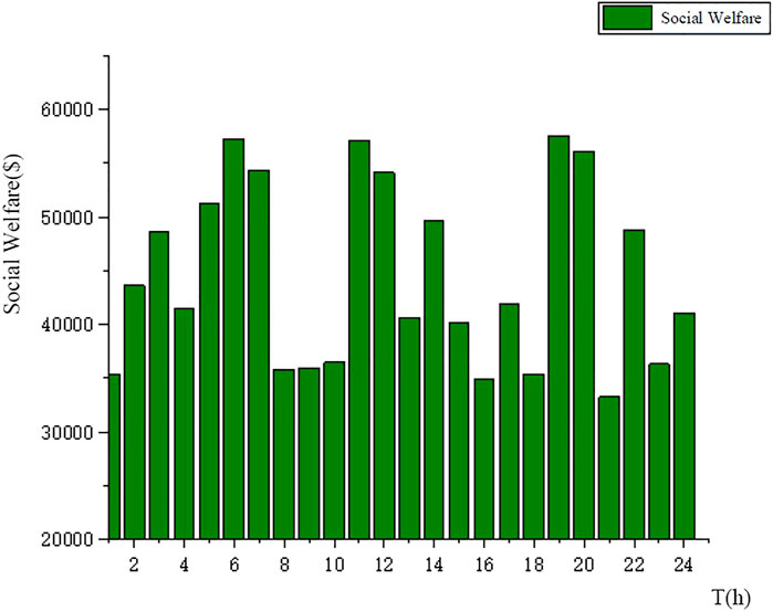
It can be seen from Table 1 that the average consumers’ weekly electricity bill is $36.85, and the average comfort index is 0.74. In this scenario, the consumers’ real-time electricity price and step tariff orders daily electricity consumption is shown in Figure 7. It can be seen that the consumers’ electricity consumption pattern has changed, and part of the load during peak period shifted to valley period. Under the premise of not disturbing consumers, the working hours of some electrical appliances are transferred to the load in the afternoon and evening hours (such as dishwashers generally start to work after meals (Dadashi-Rad et al., 2020). In order to ensure the effect of peak shaving and valley filling, the dishwasher is transferred to the load 2 hours after meals). It can be seen from Figure 8 that there is no plan for social welfare in this situation. The social welfare at this time is not very high, and the social welfare value on that day is $467,956.
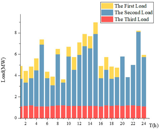
Considering scenario (2), the social welfare comparison chart is shown in Figure 9. The power distribution diagram under scenario (2) is shown in Figure 10. It can be seen that there is basically no change in part of the electricity load, and the operation basically does not change due to changes in electricity prices. The second type of electricity load is more flexible, and adjusting this type of load is the main means to ensure the economy on the basis of real-time electricity prices. The third type of load has the smallest
The smart energy planning unit could report the consumers’ electricity consumption behaviors through the regional network, which plays a corrective role in the grid load forecast. It enhances the accuracy of load forecasting for residential users. The change of parameters also has a certain impact on the optimization results. The larger the preferential ratio parameter, the weaker the consumers’ willingness to temporarily electricity consumption and the better the peak-shaving and valley-filling effect.
When the parameter
Conclusion
This paper proposes a RTP strategy. The random forest algorithm is used to forecast the load, and the fluctuation range of electricity price is determined by the fluctuation range of load. The sum of the basic electricity price and fluctuating price forms the final price. The smart energy planning unit captures the electricity price information and effectively plans the electricity consumption behavior of consumers. The optimization goal is to maximize the economy of electricity consumption and the total social welfare. The linear weighted evaluation function method is used to optimize multiobjective. Upload the consumers' electricity data to complete the two-way data transmission. The State Grid should strengthen the understanding of consumers' electricity consumption. Taking a single day as an example, the number of electrical appliances for this consumer is 13. The simulation results show that the user's weekly electricity comfort and electricity price parameters show a trend of first growth and then stability, and the reasonable setting of parameters plays an important role in the user's electricity comfort.
Data Availability Statement
The raw data supporting the conclusion of this article will be made available by the authors, without undue reservation.
Author Contributions
SW is responsible for the determination of the research direction of the paper. YZ is responsible for the editing of the text. WG is responsible for the determination of the method. AW is responsible for the data source. DL is responsible for optimized calculations. All authors contributed to manuscript revision, read, and approved the submitted version.
Conflict of Interest
SW, WG, AW, and DL are employed by State Grid Liaoning Electric Power Co., Ltd. YZ is employed by State Grid Shenyang Power Supply Company.
The remaining author declares that the research was conducted in the absence of any commercial or financial relationships that could be construed as a potential conflict of interest.
Publisher’s Note
All claims expressed in this article are solely those of the authors and do not necessarily represent those of their affiliated organizations or those of the publisher, the editors, and the reviewers. Any product that may be evaluated in this article or claim that may be made by its manufacturer is not guaranteed or endorsed by the publisher.
Abbreviations
References
Alamaniotis, M. (2020). Fuzzy Leaky Bucket System for Intelligent Management of Consumer Electricity Elastic Load in Smart Grids. Front. Artif. Intell. 3, 1–14. doi:10.3389/frai.2020.00001
Dadashi-Rad, M. H., Ghasemi-Marzbali, A., and Ahangar, R. A. (2020). Modeling and Planning of Smart Buildings Energy in Power System Considering Demand Response. Energy 213, 118770. doi:10.1016/j.energy.2020.118770
Ding, W., Yuan, J. H., and Hu, Z. G. (2005). Peak valley TOU price Decision Model Based on Customer price Response and Satisfaction. Power Syst. Auto. (20), 14–18.
Heinisch, V., Odenberger, M., Göransson, L., and Johnsson, F. (2019). Prosumers in the Electricity System-Household vs. System Optimization of the Operation of Residential Photovoltaic Battery Systems. Front. Energ. Res. 6, 145. doi:10.3389/fenrg.2018.00145
Hu, J. J. (2020). Open Sharing and Intelligent Interactive System of Power Grid Dispatching Instructions Based on Encrypted Communication Technology. Mod. Electron. Technol. 043 (002), 115–117.
Lampropoulos, I., Bosch, P., and Kling, W. L. (2012). “A Predictive Control Scheme for Automated Demand Response Mechanisms,” in IEEE Pes International Conference & Exhibition on Innovative Smart Grid Technologies, Manchester, UK, December 05, 2011-December 07, 2011. doi:10.1109/isgteurope.2012.6465647
Li, C. Y., Xu, Z., and Ma, Z. Y. (2015). Time-of-use Electricity price Optimization Model Taking into Account User Demand Response. J. Electric Power Syst. Auto. 27 (03), 11–16.
Li, Q., Li, J., Huang, Z., Fan, F., and Teng, W. (2021). A Real-Time Electricity price Decision Model for Demand Side Management in Wind Power Heating Mode. Front. Energ. Res. 9, 1–10. doi:10.3389/fenrg.2021.634603
Li, Y., Jia, Y. J., and Li, L. (2020). Short-term Power Load Forecasting Based on Random forest Algorithm. Power Syst. Prot. Control. 48 (21), 123–130.
Mohsenian-Rad, A.-H., Wong, V. W. S., Jatskevich, J., and Schober, R. (2010). “Optimal and Autonomous Incentive-Based Energy Consumption Scheduling Algorithm for Smart Grid,” in Innovative Smart Grid Technologies (ISGT), 19-21 January 2010, Gaithersburg, Maryland, USA. doi:10.1109/ISGT.2010.5434752
Reiss, P. C., and White, M. W. (2005). Household electricity demand, revisited. Rev. Econ. Stud. 72 (3), 853–883. doi:10.3386/w8687
Rothblum, U. G., and Sethuraman, J. (2008). Stochastic Scheduling in an in-forest. Discrete Optim. 5 (2), 457–466. doi:10.1016/j.disopt.2007.05.005
Venter, G., and Jaroslaw, S. S. (2003). Particle Swarm Optimization. AIAA J. 41 (8), 129–132. doi:10.2514/2.2111
Zhang, Z., Li, H., Zhao, Y., and Hu, X. (2016). “Short-term Load Forecasting Based on the Grid Method and the Time Series Fuzzy Load Forecasting Method,” in International Conference on Renewable Power Generation (RPG 2015), (IET), 17-18 Oct 2015, North China Electric Power University, Beijing, China. doi:10.1049/cp.2015.0382
Zhao, H., Ren, W. Z., and Huang, W. Y. (1997). Short Term Load Forecasting Considering Weekly Periodicity. Chin. J. Electr. Eng. 68 (03), 70–73.
Keywords: electricity market, pricing strategy, coordination optimization, peak load shifting, machine learning, random forest algorithm, multiobjective particle swarm optimization with linear weighted evaluation function method
Citation: Wang S, Zang Y, Ge W, Wang A, Li D and Tang J (2021) Data-Driven Real-Time Pricing Strategy and Coordinated Optimization of Economic Load Dispatch in Electricity Market. Front. Energy Res. 9:714951. doi: 10.3389/fenrg.2021.714951
Received: 26 May 2021; Accepted: 27 July 2021;
Published: 27 August 2021.
Edited by:
Mingyang Sun, Zhejiang University, ChinaCopyright © 2021 Wang, Zang, Ge, Wang, Li and Tang. This is an open-access article distributed under the terms of the Creative Commons Attribution License (CC BY). The use, distribution or reproduction in other forums is permitted, provided the original author(s) and the copyright owner(s) are credited and that the original publication in this journal is cited, in accordance with accepted academic practice. No use, distribution or reproduction is permitted which does not comply with these terms.
*Correspondence: Yuxiu Zang, eGl1ZGl1Yml1QDE2My5jb20=
 Shunjiang Wang1
 Yuxiu Zang