Study on Dispersion of Carbon Dioxide over the Shrubbery Region

In the carbon capture and storage (CCS) infrastructure, the risk of a high-pressure buried pipeline rupture possibly leads to catastrophic accidents due to the release of tremendous amounts of carbon dioxide (CO₂). Therefore, a comprehensive understanding of the effects of CO₂ dispersion pattern after release from CCS facilities is essential to allow the appropriate safety precautions to be taken. Due to variations in topography above the pipeline, the pattern of CO₂ dispersion tends to be affected by the real terrain features, such as trees and hills. However, in most previous studies, the dynamic impact of trees on the wind field was often approximated to linear treatment or even ignored. In this article, a computational fluid dynamics (CFD) model was proposed to predict CO₂ dispersion over shrubbery areas. The shrubs were regarded as a kind of porous media, and the model was validated against the results from experiment. It was found that shrubbery affected the flow field near the ground, enhancing the lateral dispersion of CO₂. Compared with that of the shrub-free terrain, the coverage area of the three shrub terrains at 60 s increased by 8.1 times, 6.7 times, and 9.1 times, respectively. The influence of shrub height and porosity on CO₂ dispersion is nonlinear. This research provides reliable data for the risk assessment of CCS.

Highlights

CFD model of heavy gas dispersion considers shrubs under

Sensitive analysis on arrangement of shrubs on heavy gas dispersion

Influence of shrub height and porosity on CO₂ gas concentration is nonlinear

Introduction

Burning fossil fuels leads to the enormous amounts of emission of carbon dioxide (CO₂), which increases the concentration of CO₂ in the atmosphere inevitably and contributes to the “greenhouse effect” (Peters et al., 2013). Worldwide, due to continuous industrial development, fossil fuels are still in high demand (IEA 2018) in the foreseeable feature; therefore, substantial attention has been paid to technologies that may reduce excessive concentrations of CO₂ in the atmosphere, and several technical methodologies need to be implemented. It is widely accepted that the deployment of carbon capture and storage (CCS) is one of the most promising and feasible methodologies for reducing artificial CO₂ emissions (Metz et al., 2005). CCS involves capturing CO₂ emitted by large-scale anthropogenic CO₂ sources (e.g., fossil fuel power plants) and transporting it to an isolated geological formation for storage, instead of being discharged into the atmosphere (Liu et al., 2015). Furthermore, the renewable energy industry is developing rapidly currently; however, if no effective treatment is carried out correspondingly such as CCS, the final carbon emission in numerous new energy production processes may even exceed that of fossil fuel (hydrogen production from natural gas, etc.). Pressurized pipeline application constitutes a part of the CCS chain, which is regarded as the most practical and economical land transportation methodology for the subsequent storage of large amounts of CO₂ collected from CO₂ source such as coal-fired power plants. The delivery pressure of this type of pipeline usually ranges between 10 and 20 MPa and their length can be up to hundreds of kilometers.

However, CCS technology remains at the developing stage, and the safety issue is of paramount significance. Corrosion, material defects, operator errors, and earthquakes may affect the safety of CO₂ transportation pipelines, causing inevitable rupture and leakage (Gale and Davison 2004). Notably, CO₂ is heavier than air; thus, it is more likely to sink and accumulate in low-lying areas when the transport pipeline is broken, making its spread challenging. Also, CO₂ is an asphyxiant gas, and at high concentrations, excessive CO₂ inhalation may result in coma or even death for humans and animals, which poses a substantial danger to nearby organisms (Mazzoldi et al., 2008). In addition, the features of colorless and not flammable may bring about CO₂ leakage difficult to detect. Therefore, in order to protect humans and animals from the possible harmful effects caused by pipeline accidents, it is necessary to leave a sufficient safety distance between densely populated areas and high-pressure CO₂ pipelines (Lipponen et al., 2011; Liu et al., 2012). To predict such distance, it is necessary to develop a reliable CO₂ dispersion model after the event of accidental release.

Over the past few decades, various atmospheric dispersion models have been performed, such as Accident Damage Analysis Module (ADAM) (Fabbri et al., 2017; Fabbri and Wood 2019; Fabbri et al., 2020), ALOHA (NOAA/EPA 1992) [based on DEGADIS (Havens and Spicer 1990)], DRIFT (Gant et al., 2018; Gant et al., 2021), the ESCAPE model (Expert System for Consequence Analysis and Preparing for Emergencies) (Kukkonen et al., 2017), and the HPAC/SCIPUFF (Hazard Protection Assessment Capability/Second-Order Closure Puff) (Simpson et al., 2020). With improved computational resource availability, the computational fluid dynamics (CFD) models have gradually become the most popular model.

CFD models are based on the conservation principle of the Reynolds-averaged Navier–Stokes (RANS) equation to carry out complex mathematical descriptions, thus allowing the integration of complex geometrical or physical and chemical phenomena. They enabled to be established to solve the three-dimensional space and time of fluid mechanics equations and therefore can accurately and in detail describe the complex geometrical shape of the flow (Ahmed et al., 2016; Liu et al., 2016; Efthimiou et al., 2017; Liu et al., 2017) and is increasingly used in the study of hazardous gas dispersion over the complex terrain (Sklavounos and Rigas 2006; Luketa-Hanlin et al., 2007; Gavelli et al., 2008; Tauseef et al., 2011; Hsieh et al., 2013; Tan et al., 2018).

Typically, dispersion patterns over an isolated obstacle or a group of obstacles have been studied comprehensively conducted by CFD modeling (Tominaga and Stathopoulos 2010; Takano and Moonen 2013; Kumar et al., 2015; Stabile et al., 2015; Bijad et al., 2016; Liu et al., 2016; Wingstedt et al., 2017; Liu J. et al., 2019; Ding et al., 2020; Ryan and Ripley 2020; Wang J. et al., 2021). These studies were usually designed to validate the performance of CFD in simulating the dispersion of pollutants around the obstacle/obstacles. In such terrains, pollutants may be trapped in the street “canyons” formed by buildings (obstacles) and also in the “wake” of buildings. The effects of pollutant transport models and inflow conditions, canyon structure and building size, were studied. Since the objective of the gas dispersion model is to predict the time-varying dispersion of pollutants in the real environment, it becomes necessary to consider geometrical variations within the area of interest because the wind field is inherently associating to the layout of buildings. Meroney (2010) used the CFD code ANSYS Fluent to simulate the dispersion of CO₂ in an urban environment with single or multiple building obstacles. Their study showed that a heavy gas cloud collapsed toward the ground rapidly and spread radially. Then, the cloud clusters were stratified due to the difference in density and preserved a pancake or flat appearance for a long-distance downwind. However, when the cloud was blocked by obstacles, the stratification was weakened and vertical movement was allowed. In the wake of a single obstacle or an array of buildings and owing to the low wind speed between the buildings, high concentrations of gas may continue to exist, delaying the dispersion time. Liu et al. (2016) developed a CFD model to study CO₂ dispersion over two types of terrain. It was found that the CFD model was able to produce relatively accurate concentration estimations. Also, terrain features and weather conditions had a great impact on the character of CO₂ dispersion. Hsieh et al. (2013) established a CFD model for dense gas dispersion based on the RANS method and analyzed the influence of buildings and complex terrain on the dispersion pattern. Based on the Boussinesq method, they derived the buoyancy term. This model can be used to provide the information needed for quantitative evaluation of the potential risks to the public caused by accidental or malicious release of CO₂ from CCS-related infrastructure.

From a modeling capability perspective, CFD models can simulate complex physical processes, such as heat and mass transfer, in a complex three-dimensional (3D) calculation domain. Moreover, CFD models allow the calculation of variable physical properties of the fluid, turbulence modeling, chemical reactions, creation of accurate descriptions of turbulent mixing, 3D plumes, and the geometric flow field required to disperse fluids. However, numerous previous CFD investigations have proven that the description of the turbulence model has a great influence on the predicted precision in reproducing heavy gas dispersion. This is especially true for real complex terrain. Thus, it is particularly important to select an appropriate turbulence model. Toja-Silva et al. (2017) compared differential column measurements (Chen et al., 2016) with CFD simulation. They used the RANS turbulence model based on the open-source CFD software package OpenFOAM. The accuracy of the model was validated by the comparison between the CO₂ prediction of column-averaged dry-air mole fraction (XCO₂) and the experimental measurement results. Different turbulent Schmidt numbers were compared, and Sct = 0.6 was identified as the most adequate for being used in CFD simulations of CO₂ emissions from power plants in urban areas.

In recent years, a remarkable number of efforts have been implemented to improve the ecological environment and reduce the soil losses caused by floods using afforestation and the restoration of forest vegetation. Therefore, city suburbs now usually cover not only natural vegetation but also newly planted trees. The behavior of flows over or through tree areas has become a hot area of research in numerous fields. In what relates to the influence of plant canopies on atmospheric wind environment, the analysis has been carried out. Trees are known to reduce temperature, increase humidity, prevent wind and dust, cause particle deposition (Vos et al., 2013; Jeanjean et al., 2017; Buccolieri et al., 2018), as well as resuspension (Nowak et al., 2013; Hong et al., 2018), canopy transpiration (Hagishima et al., 2007), and create shadow effects (Sabatino et al., 2015). They also reduce energy consumption and alleviate air pollution notably (Gallagher et al., 2015; Gromke et al., 2016; Li et al., 2016). The deposition of particulate matter on plant surfaces helps remove pollutants from the atmosphere, reducing their concentration. However, trees themselves act as porous obstacles to reduce wind speed, airflow, decrease air exchange, and probably lead to higher pollutant concentrations primarily due to pressure and viscous drag forces. In the foundation of the understanding of the flow within and around trees, there was an extensive numerical CFD study on the effects of vegetation on the atmospheric wind environment, which were often carried out using large eddy simulation (LES) and RANS methods. Such CFD methods ensured a true representation of flow dynamics in complex environments (e.g., urban canopies covered by vegetation) and produced high-resolution flow fields. Buccolieri et al. (2009) studied the aerodynamic effects of tree-lined greening on the flow field in urban streets and canyons, through wind tunnel tests and numerical simulations. In addition, they analyzed the dispersion process of traffic source pollutants. The CFD code ANSYS Fluent was employed to achieve a 3D numerical simulation for the flow and dispersion of traffic exhaust gas in a tree-planted city street canyon with a width to building height aspect ratio of 2. It was deduced that street trees have a notable impact on pollutant concentrations in street canyons. Moonen et al. (2013) conducted CFD simulations with the LES model to quantitatively predict pollutant dispersion potential. The model performed better in predicting a leeward canyon than in a windward wall, and the system performance near the end of the street canyon was better than that in the center of the street canyon. The presence and density of trees in the street canyon hardly systematically affect the overall model performance. This model confirmed the applicability of the COST (COST Action 732, 2007a; COST Action 732, 2007b; COST Action 732, 2007c; COST Action 732, 2010) recommendation and supported the premise that it is necessary to combine qualitative and quantitative techniques to assess the applicability of a specific model for a specific purpose. Hefny Salim et al. (2015) employed three different methods to simplify the role of urban trees in the numerical simulation of wind fields, emphasizing the impacts of trees on pollutant dispersion, air quality assessment, and wind environment comfort research. Compared with the case without trees on the streets, the results obtained by the explicit porous medium method demonstrated that trees reduced the wind speed in the street canyon. Barbano et al. (2020) used a simplified CFD tool (QUIC) to simulate and evaluate the average wind and turbulence fields of a vegetated urban neighborhood. By comparing the simulation results with and without trees, they found that trees could reduce airflow by restricting local circulation and reducing the intensity of turbulence. The results showed that the blocking effect of trees was dominant in both the average and turbulent flow fields. Both types of flow fields were sensitive to the density of obstacles (e.g., buildings and trees). Weakly unstable conditions and thermal stratification reduce the quality of the simulation results, not allowing the QUIC model to account for local airflow changes produced exclusively by trees; however, the model can capture the feature of near-neutral conditions and vertical wind directions well.

Shrubs are short woody plants with multiple trunks and are indispensable in many ecosystems. Shrubs tend to distribute more widely than trees (Myers-Smith et al., 2015). Although both trees and shrubs may exist in forest landscapes, most studies focus on tree species and their response to weather change (Morales et al., 2012; Götmark et al., 2016). Previous studies have shown that shrubs have been more sensitive to weather change than trees (Morales et al., 2012; Pellizzari et al., 2017). The flow patterns through or around the shrubs are complicated by the presence of bleed flows and displaced flows. Dong et al. (2008) measured and analyzed the flow field around shrubs with different densities in the wind tunnel. The results showed that porosity was an important factor affecting the flow field structure around shrubs. When the density of the shrub was less than the critical density of 0.08, the airflow through the shrub was obviously strengthened, while the updraft on the windward side rapidly weakens, and the seepage flow was dominant; when the value of the shrub density was equal to or exceeded the critical density, the updraft was formed on the windward side and a large vortex structure rotating clockwise appears on the leeward side. Wu et al. (2015) simulated the flow field around the shrub windbreaks in the wind tunnel. The results show that the average velocity field around the shrub can be divided into the front deceleration zone, the upper acceleration zone, the rear vortex zone, and the recovery zone downwind of the vortex zone. The protection effect of shrub windbreak varied with the change of wind speed and was affected by its structure. The shrub windbreaks with more complex layout can reduce wind speed more effectively, extend sheltering distances, and have better protective effects than simple shrub windbreaks. However, there have been few studies linking the arrangement of shrubs and their impact on heavy gas dispersion patterns to date. To quantify the risks of heavy gas dispersion, it is essential to construct heavy gas dispersion models that consider the effects of shrubs on complex terrain.

The primary purpose of this study is to evaluate the influence of complex shrubland topography on the CO₂ dispersion characteristics. The CFD model was carried out to simulate CO₂ dispersion over shrubland, and shrubs were regarded as porous media. Based on previous research, the correctness of the CFD model presented herein was verified by comparing its prediction with a full-scale blasting test data and the experimental measurement data of trees (Japan Architectural Society). The rest of this article is organized as follows: Numerical Methods introduces the numerical methods; Computational Fluid Dynamics Model explains the CFD model construction and model validation; and Results and Discussion present the influence of the location, height, and porosity of shrubs on the CO₂ dispersion characteristics. This research provides a reliable method for predicting heavy gas dispersion in case of the leakage of high-pressure CO₂ pipelines under complex shrubland terrain and the analysis procedures and results can be utilized for CCS risk assessment.

Numerical Methods

To predict the CO₂ dispersion characteristics released from high-pressure pipelines, we used CFD software ANSYS Fluent 15.0 (ANSYS 2011a) in current work. Considering the compromise between computational time and accuracy of the model, the RANS model was employed. The RANS model involves solving the conservation equations of mass, momentum, and energy. Apart from the conservation equations, turbulence and component transportation equations solve the complex problems of 3D turbulence field changes, time-varying rate of mass change of each component, and spatial distribution of concentration of different species. Shrubs were treated as kind of porous media, and their influence on the entire turbulent field was explored.

The equations used for continuity, energy conservation, and momentum were as follows:

Continuity equation

$\frac{\partial \rho }{\partial t}+\nabla \cdot \left(\rho \overrightarrow{\nu }\right)=0,(1)$

Energy equation

$\frac{\partial \left(\rho E\right)}{\partial t}+\nabla \cdot \left[\overrightarrow{v}\left(\rho E+p\right)\right]=\nabla \cdot \left[k_{eff}\nabla T-{\displaystyle \sum }_i{h}_i\overrightarrow{J_i}+\left({\overline{\tau }}_{eff}\cdot \overrightarrow{v}\right)\right],(2)$

Momentum equation (Navier–Stokes equation)

$\frac{\partial \left(\rho \overrightarrow{v}\right)}{\partial t}+\nabla \cdot \left(\rho \overrightarrow{\nu }\overrightarrow{\nu }\right)=-\nabla p+\nabla \cdot \left(\overline{\text{τ}}\right)+\rho \overline{g}+F_d,(3)$

$\overline{\tau }=\mu \left[\left(\nabla \overrightarrow{\nu }+\nabla {\overrightarrow{\nu }}^T\right)-\frac{2}{3}\nabla \cdot \overrightarrow{\nu }I\right],(4)$

where $\rho$, $\overrightarrow{\nu }$, and p are the density, velocity vector, and pressure, respectively; $\rho \overline{g}$ represents the gravitational force per unit volume; F_d is source term, and its specific content is shown in Eq. 7; $\overline{\tau }$ is the stress tensor (described in Eq. 4), where μ is the dynamic viscosity; E represents the total energy; and k_eff, T, h_i, and $\overrightarrow{J_i}$ are the effective thermal conductivity, temperature, specific enthalpy of species i, and diffusion flux, respectively.

Turbulence Equations

An improved standard k–ε model characterized by a high Reynolds number was utilized for design selection, parameter study, and the initial iteration (Smagorinsky 1963; Launder, 1972). Turbulent kinetic energy k and its dissipation rate ε were obtained from the following transport equations:

$\frac{\partial \left(\rho k\right)}{\partial t}+\frac{\partial }{\partial x_i}\left(\rho k{u}_i\right)=\frac{\partial }{\partial x_j}\left[\left(\mu +\frac{{\mu }_t}{{\sigma }_k}\right)\frac{\partial k}{\partial x_j}\right]+G_k+G_b-\rho \epsilon -Y_M+S_k,(5)$

$\frac{\partial \left(\rho \epsilon \right)}{\partial t}+\frac{\partial }{\partial x_j}\left(\rho \epsilon u_i\right)=\frac{\partial }{\partial x_j}\left[\left(\mu +\frac{{\mu }_t}{{\sigma }_{\epsilon }}\right)\frac{\partial \epsilon }{\partial x_j}\right]+C_{1\epsilon }\frac{\epsilon }{k}\left(G_k+C_{3\epsilon }{G}_b\right)-C_{2\epsilon }\rho \frac{{\epsilon }^2}{k}+S_{\epsilon },(6)$

where G_k is the turbulent kinetic energy due to the average velocity gradient; G_b is the turbulent kinetic energy due to buoyancy; Y_M represents the contribution of wave expansion to the total dissipation rate in compressible turbulence; C₁, C₂, and C₃ are constants; σ_k and σ_ε are the turbulent Prandtl numbers for k and ε, respectively; and S_k and S_ε are the user-defined sources. The standard coefficient was used to build the turbulence model, and the Boussinesq approximation method was applied to model the buoyancy effect.

In the CFD simulation process, it is particularly important to select the appropriate geometric model and physical model. Liang et al. (2006) used three different canopy shapes: the pyramid crown model, the truncated body of the pyramid crown model, and the cuboid crown model to study the influence of shrub on atmospheric flow. The results showed that the canopy shapes affected the results distinctly and the cuboid canopy model provided the best consistency with the experiment data, also with less computational time. Therefore, in the current simulation, the cuboid canopy model is selected to describe the shrub’s shape and treat it as a porous medium due to the complex microstructure of the shrub. The existence of shrubs increases the turbulence intensity around the shrub region. It reduces the wind speed downstream of the shrub region, so an additional moment source term F_d was added to the momentum in Eq. 3:

$F_d=-C_{d}a{u}_i\left|U\right|,(7)$

$\left|U\right|={\left({\displaystyle \sum _{i=1}^2{u}_i^2}\right)}^{\frac{1}{2}},(8)$

where C_d is the drag coefficient of shrubs (values are shown in Table 1); a is the leaf area density (m²/m³); u_i is the velocity component (m/s); and |U| is the average wind speed (m/s).

TABLE 1

TABLE 1. Dimensionless constants.

In the standard k–ε equation, owing to the influence of the shrub and wind shear in the airflow produces turbulence, and the turbulent energy of the surrounding flow field is attenuated. Therefore, additional source terms S_k and S_ε in Eqs. 9, 10 were defined as follows:

$S_k=C_{d}a\left({\beta }_p{\left|U\right|}^2-{\beta }_d\left|U\right|k\right),(9)$

$S_{\epsilon }=C_{d}a\left(c_{\epsilon 4}{\beta }_p{\left|U\right|}^2\frac{\epsilon }{k}-c_{\epsilon 5}{\beta }_d\left|U\right|\epsilon \right).(10)$

The dimensionless constants β_p, β_d, c_ε4, and c_ε5 are shown in Table 1.

Species Transport Equation

The species transport equation of components was carried out to calculate the spatial distribution of concentration for each species. This equation is expressed as the time-varying change rate of a component mass in the system equal to the sum of the net diffusion flux through the system interface and the generation rate of the component by a chemical reaction. Two components were considered in the current study: CO₂ and air. As there is no chemical reaction between CO₂ and air, the mass change rate of CO₂ or air in the system is equal to its net diffusion flow flux. The mass fraction of each species was predicted by solving the convection–diffusion equation and using the species transport model (ANSYS 2011a):

$\frac{\partial \left(\rho Y_i\right)}{\partial t}+\nabla \cdot \left(\rho \overrightarrow{\nu }{Y}_i\right)=\nabla \cdot \overrightarrow{J_i}+R_i+S_i,(11)$

where $R_i$ is the net productivity of the species; ρ is the density of CO₂ or air in the system; $Y_i$ is the mass fraction of species i, and the sum of fractions of all species equals 1; $\overrightarrow{\nu }$ and $\overrightarrow{J_i}$ are the gas diffusion velocity vector and diffusion flux, respectively; and $R_i$ and $S_i$ are the net production rate of species i and the additional production rate caused by the user-defined source term and discrete term, respectively. Since no chemical reaction occurs, both $R_i$ and $S_i$ were set to 0.

In the dispersion model, the viscosity and thermal conductivity of CO₂ were set to 1.37 × 10^–5 kg⋅m^-1⋅s^-1 and 0.013 W⋅m^-1⋅K^-1, respectively, and CO₂ was considered as an incompressible ideal gas and temperature T (K) as follows:

$\rho =5.3105-0.01432T.(12)$

Additionally, in heavy gas dispersion modeling, it is crucial to describe the wind speed precisely as it directly affects the air distribution. In the atmospheric boundary layer, the wind speed usually decreases with a reduction in height due to the friction effect of the ground. The wind inlet velocity is specified by a power-law correlation to express the atmospheric boundary layer. The velocity distribution defined by Peterson and Hennessey (1978) is most widely used to describe the vertical wind profile near the ground:

$u=u_r{\left(\frac{z}{z_r}\right)}^{\alpha },(13)$

where u is the wind velocity at altitude z; u_r is the reference wind speed measured at reference altitude Z_r; and wind shear index α is related to atmospheric stability, geographical environment, and other factors. The parameters used in the current work are consistent with those used in previous studies (Wang H. et al., 2021).

Computational Fluid Dynamics Model

Determination of Release Source and Computational Domain

In our previous study (Wang H. et al., 2021), we evaluated the performance of computed results of CO₂ dispersion over a flat terrain with the measures from the full-scale test carried out by the 2016 Australian CO₂ pipeline safe transportation project (Liu X. et al., 2019). Rather than the most of other “model” tests, this full-scale test provided the data represented a more realistic release scenario that CO₂ release from a buried high-pressure pipeline due to a crack induces a fracture propagating. As the test did not offer the information of all the terrain features, the influence of surrounding trees or shrubs on dispersion characteristics was ignored in the CFD model. However, trees or shrubs pattern, such as heights, porosities, and relative position from the CO₂ release source, may lead to a great impact on the surrounding flow field. This is probably the reason for the deviation between the measured and CFD resulted. Therefore, in current work, the CFD model was improved and the incorporated porous model represented the influence of trees or shrubs to provide a comprehensive view of the possible consequences of a full-scale pipeline fracture.

CO₂ dispersion over a flat featureless terrain was set as a reference case (case0), and the box-shaped computational domain was shown in Figure 1A. Figures 1B–D show the analogous computational domains with shrubs arranged in different relative positions. The domain enclosed with six boundaries, specifically the ground (in brown), wind inlet, left, right, outlet, and top. The strip shrub regions were shown in green. The size was 1,500 m (long) × 800 m (wide) × 400 m (height), and the wind inlet was located in 200 m upstream of CO₂ release source. The exit of the calculation domain (outlet) was located sufficiently far downstream from the release source; therefore, the backflow effect can be ignored. The size of the computational domain was sufficiently large and met the requirements for the dispersion simulation.

FIGURE 1

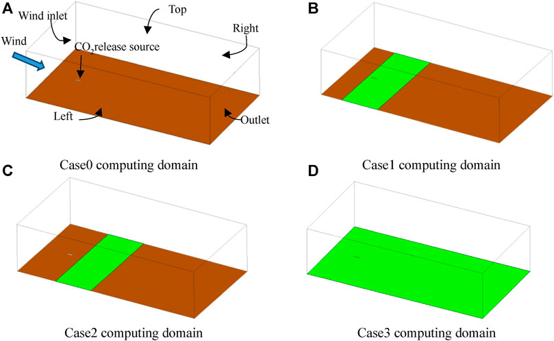
FIGURE 1. Four cases of computing domain.

A vertical release perpendicular to the wind direction was considered. The environmental parameters of the wind parameters were consistent with the test conducted by the Architectural Society of Japan and were used for comparison (AIJ, 2020; Mochida et al., 2008). The specific parameters of the four simulated cases are listed in Table 2. Case0 is the basic topography of uncovered shrubs (Figure 1A); case1 is the topography of strip shrubs covered with release sources (Figure 1B) and strip shrubs are covering the release source. To analyze the impact of shrub height and porosity on gas dispersion, the heights of the shrubs in case1 are adjusted to 0.5, 1, and 1.5 m, respectively, and the porosities are 0.3, 0.6, and 0.9. The smaller the porosity, the greater the wind resistance. Case2 is also a strip shrub terrain. The strip shrub is located at 100 m behind the release source, which is different from case1. Case3 is a terrain that is covered entirely with shrubs. The heights of shrubs in case2 and case3 are both 1 m and the porosities are both 0.9.

TABLE 2

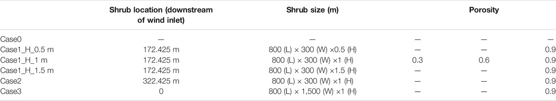
TABLE 2. Specific parameters of the four computed cases.

ANSYS-ICEM is applied to reasonably generate the hexahedral structure mesh. The grid growth rate is fixed within a certain range according to previous research (Wang H. et al., 2021), and the numbers of grid for different terrains are between 3 and 4 million.

Boundary and Initial Conditions

The numerical simulation was divided into two stages: 1) steady-state simulation and 2) transient simulation. The initial wind flow field over the specified terrain was obtained using a steady-state simulation, without the emission of CO₂. The transient simulation was based on the steady-state initial flow field as well as introducing CO₂ from the “source,” and CO₂ dispersion was simulated over time. Additionally, the simulation of case0 was based on a full-scale test (Liu X. et al., 2019), and the CFD models have been previously validated (Wang H. et al., 2021). In that case, CO₂ was simulated to dispersers over a flat featureless terrain. The numerical simulation used herein was based on the same time-varying release source inlet conditions as that in the previous study. Other cases were improved on this basis. The CFD simulation condition settings are presented in Table 3.

TABLE 3

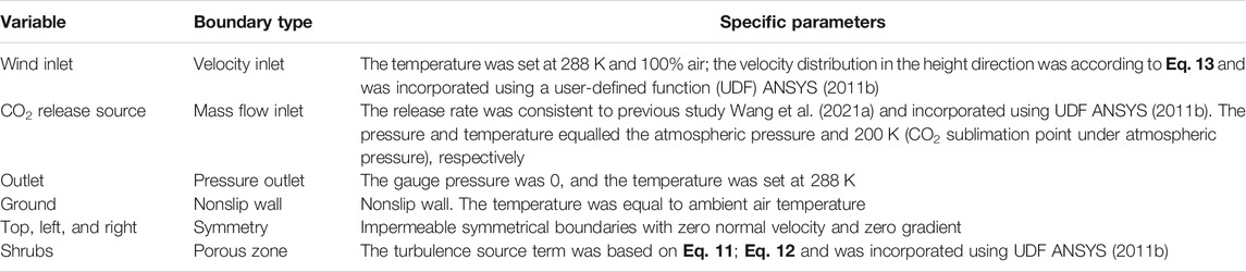
TABLE 3. Boundary condition.

Porous Media Model Verification

To evaluate the performance of the proposed porous model, flow field data from the experiment carried out by the Architectural Society of Japan were used for comparison (AIJ, 2020; Mochida et al., 2008). All the parameters, including inlet conditions and monitoring point distribution were derived from and according to with the experiment. The settings for the porous media were based on Eqs. 8, 10, 11 to obtain the corresponding UDF (ANSYS 2011b).

Table 4 shows the comparison between the measured wind speed values (AIJ) and those from the numerical simulation. As the monitoring point was located on the leeward side of the tree, the influence range and deceleration effect by the tree on the wind speed changed owing to the relative distance. Overall, the simulation results of the velocity profile were consistent with that from the experimental values, especially when the value of X/H ranged between 0.5 and 3; the data were consistent, and the relative error was small. It is worth noting that when the value of X/H was 2, the data fit was slightly worse in Figure 2. This may attribute to the underestimation of the influence range and deceleration effect of the wind speed by trees. Generally speaking, the adopted porous model could accurately simulate the influence of trees on the flow field, thereby ensuring the accurate prediction of the entire model.

TABLE 4

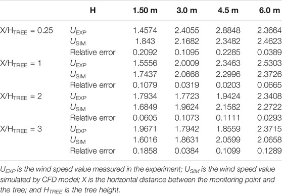
TABLE 4. Comparison of wind speed measurement (AIJ) and numerical simulation.

FIGURE 2

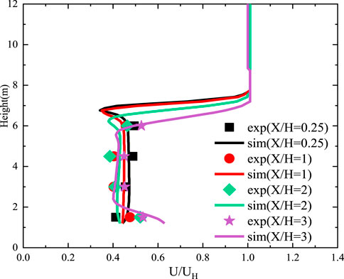
FIGURE 2. Comparison of wind speed measurement (AIJ) and numerical simulation.

Results and Discussion

Previous studies (Liu et al., 2016; Wang H. et al., 2021) indicated that the dispersion pattern of CO₂ under the condition of large-scale turbulence was dominated by convective diffusion, whereas molecular diffusion can be negligible. Initially, the effect of gravity was significant, and the gas collapsed to form a heavy gas cloud promptly. Then, the CO₂ cloud was gradually diluted by ambient air, resulting in decreased density and apparent lateral dispersion. With time, the heavy gas cloud was passively dispersed by the wind and was further diluted by air. Eventually, the effects of gravity and buoyancy achieved balance. The convection diffusion of heavy gases was affected by terrain features notably, such as obstacles, and other landscape aspects. The natural shrubs in the environment were mostly low. Since their heights quite differed from that of buildings or trees, the shrubs predominantly affected the flow field near the ground. When the location, height, porosity, and other profiles of the shrubs changed, the flow field, direction of CO₂ convection and dispersion, concentration at different locations, and consequence distance were all modified correspondingly.

Influence of Shrubland Relative Location

Figures 3A–D show the initial flow field covering the shrubs for cases 0–3 (a cross section parallel to the ground with a height of 1 m). The green region represents the zone covered by shrubs, whereas the yellow is the flat featureless region. When shrubbery cover the release source (case1), the flow field near the release source is prone to eddy currents (Figure 3B). The shrub coverage areas chosen for case1 and case3 differ substantially in terms of streamline distribution (as shown in Figures 3B,D). In terms of case2, the shrub region boundary is located 322.5 m downstream of the wind inlet and 100 m away from the center of the release source. It should be noted that in a flat terrain without shrubs, the streamlines are mostly parallel to the wind direction and approximately perpendicular to the streamlines in the shrub area (especially at the wind inlet). Whereas in the shrubland-covered area, the streamlines are mostly perpendicular to the wind direction or have a clear angle with the wind direction. The turbulent flow around the porous medium area is enhanced, the wind speed is reduced, and obvious eddies could be observed. At the junction of flat terrain and shrubland terrain, the direction of the streamline changes suddenly, where the turbulence changes more obviously.

FIGURE 3

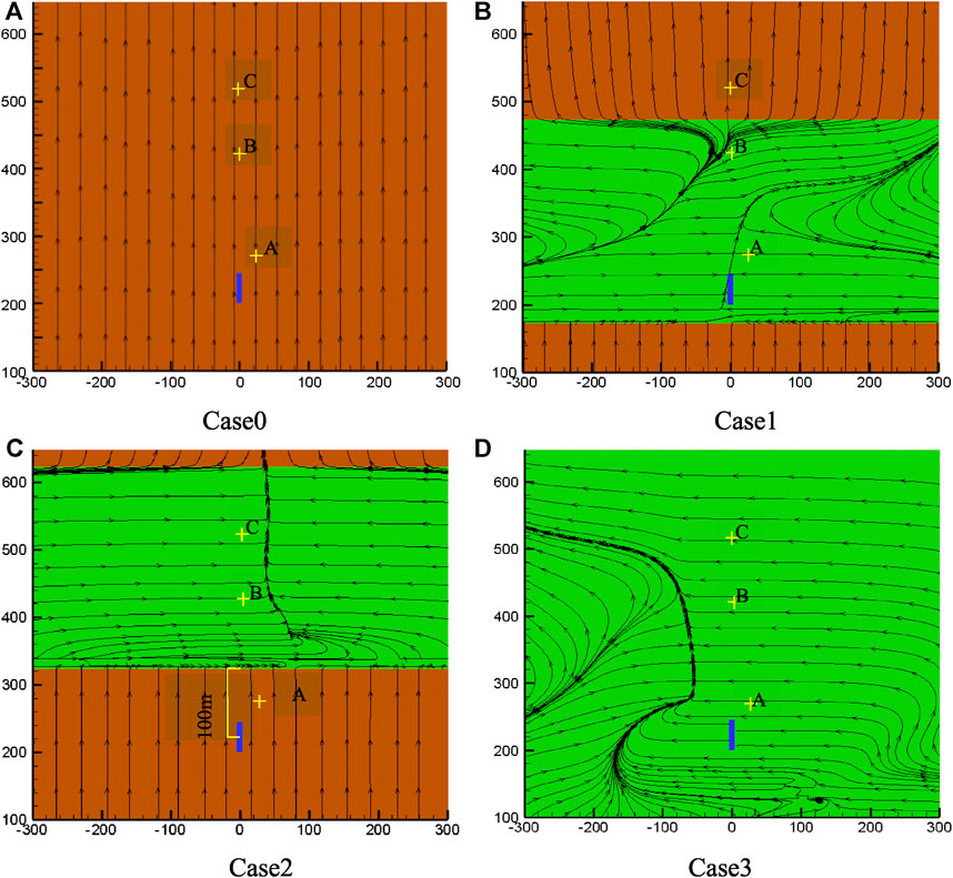
FIGURE 3. Top view of the initial flow field created in the shrubbery for three different cases.

Figures 4A–C show the time-varying CO₂ concentration at 1 m elevation at points A (50 m), B (200 m), and C (400 m). The locations of the monitoring points of the three cases are the same; points A, B, and C are, respectively, located at 50, 200, and 400 m downwind from the center of the release source. At point A (Figure 4A), the CO₂ concentration varied rapidly under all three shrubbery-covered scenarios. Clearly, when the shrubbery covers the release source (case1), the CO₂ concentration peaked three times successively. The highest CO₂ concentration reaches 29.6% in terms of case1, 5.3% in case2, and only 2.1% in case3. Also, the CO₂ concentration in case1 covered by shrubbery is 4.5% higher than that in case 0. There is no doubt that such a discrepancy is due to a significant change in the nearby flow field when a 1-m high shrub is located 100 m behind the release source (Figure 4B), thereby increasing the gas concentration. However, as for case2, unlike the other two cases where shrubs cover the release source (case1 and case3), shrubs represent porous media and substantially impact the wind environment around the release sources, diluting the CO₂ concentration and making it much lower at point A than that in a forest without shrubs (case0). It can be seen from Figure 4B that the CO₂ gas cloud in case2 disperses to point B at 39.5 s, and is the fastest case, whereas in case3 and case1, CO₂ disperses to point B at 59.2 and 65.3 s, respectively. It is observed that when the shrub region covers the release source (case1 and case3), the cloud dispersion speed slows down and the gas cloud reaches point B later. The results also show that from 104.6 s until 300 s, the concentration value at point B remained within the range between 0.5 and 1% (case1 and case3), and the overall CO₂ volume fraction vs. time curves fluctuate unobvious. Specifically, when CO₂ cloud in case2 disperses to point B, the first peak concentration of 2.3% appears at 47.6 s. Due to the existence of a certain distance between the shrub region and the release source, the effect of shrub retardation on gas dispersion is not obvious. After reaching the first CO₂ concentration peak of 0.87% and appeared at 75.1 s in case3, the concentration first decreases and then increased to the second peak. It can be seen from this that for point B, there is little difference in the delaying effect of CO₂ gas between the whole ground cover shrub (case3) and the shrub cover at the center of the release source (case1). At point C (Figure 4C), the concentration of CO₂ in case1 raised more rapidly compared with those in case2 and case3, and the maximum concentration of 1.39% lasted for approximately 19 s.

FIGURE 4

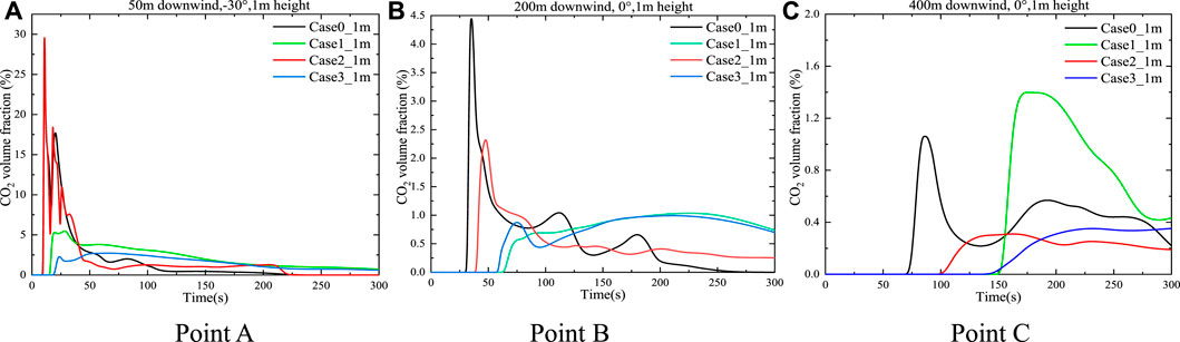
FIGURE 4. CO₂ concentrations at different locations based on the distance from the center of the CO₂ release source.

Due to the strong Joule–Thomson effect during high-pressure CO₂ expansion, the temperature of CO₂ will drop sharply after leaking from a high-pressure pipe; therefore, dry ice is formed, which will sublimate quickly, thus forming a low-temperature area near the nozzle. After pipeline rupture, CO₂ leakage flow rate also changes significantly over time. The relationship between CO₂ flow rate and time measured in the real full-size blasting experiment is as follows:

$m=C_1\left({\text{e}}^{C_{2}t}-{\text{e}}^{C_{3}t}\right),(14)$

where t was time, and C₁, C₂, and C₃ are coefficients controlling the release rate. According to the data measured from the full-scale blasting experiment (Liu X. et al., 2019), the values of these three parameters were 75300 kg s^-1, −1 s^l, and −10 s^-1, respectively.

The National Institute of Occupational Safety and Health (NIOSH) states that the long-term exposure to 0.5% (5,000 ppm) concentration of CO₂ will cause dizziness, restlessness, and helplessness. In addition, NIOSH pointed out that exposing people to a CO₂ concentration of 4% (40,000 ppm) will issue in very rapid breathing, confusion, and even coma (NIOSH 2005). Therefore, in the following analysis, the consequence distance was determined as the distance away from pipe rupture contained by the concentration envelope corresponding to this concentration level of 4% and it is called CD-4.

Figures 5–8 show the CD-4 obtained in four different terrains at different times. Under all terrain conditions, the CO₂ cloud clusters had a certain height at the initial stage of the release. As CO₂ gas is released within 12 s [corresponding to the blasting experiment (Wang H. et al., 2021)], the cloud clusters begin to collapse because of the high cloud density. The release sources in case0 and case2 are not covered by shrubs, whereas there are different distances from release sources to the shrub covering boundary as for case1 and case3. Thus, in the initial stage, lateral dispersion of CO₂ for case0 and case2 is not as obvious as that for case1 and case3. Simultaneously, the coverage areas of the CD-4 for case0 and case2 are relatively smaller at 10 s (Table 5).

FIGURE 5

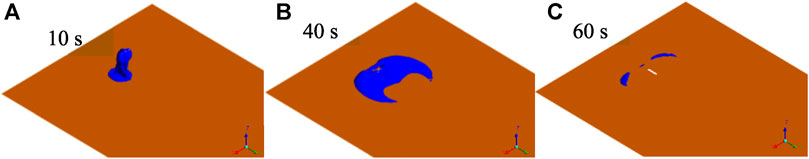
FIGURE 5. CD-4 at different time (case0).

FIGURE 6

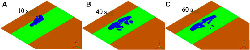
FIGURE 6. CD-4 at different times (case1).

FIGURE 7

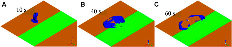
FIGURE 7. CD-4 at different times (case2).

FIGURE 8

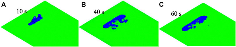
FIGURE 8. CD-4 at different times (case3).

TABLE 5

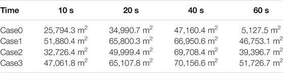
TABLE 5. CD-4 calculated at different time points of four terrain types.

In the initial dispersion stage, compared with those in case0 and case0, the lateral consequence distances in case1 and case3 became more obvious. This is because the shrub had a strong blocking effect on the wind field around the release source and delayed the formation of heavy gas clouds. It is worth noting that the dispersion of clusters may make rescue operations more difficult, especially when the coverage area is extensive, and there are high CO₂ concentrations.

In general, regardless of the thermal gradient effect (related to the air stability level) on the generation or suppression of turbulence, shrubs have a substantial impact on the near-surface flow field and are more likely to produce mechanical turbulence than shrub-free terrain. When shrubs cover the release source, the lateral dispersion of heavy gas cloud clusters becomes more significant. It is indicated that the cloud cluster grows larger and the dispersion duration is prolonged.

Effect of Shrub Height

There are a series of types of shrubs, and their heights varied from 0.1–6 m, while the common shrub heights in suburban woodlands are 0.5–1.3 m (Zhang 2009). It is valuable to study the effect of shrub height on the dispersion pattern. The reference wind speed during the simulation of dispersion is 5 m s⁻¹. Three types of shrubs with heights of 0.5, 1, and 1.5 m are considered and termed Terrain I, Terrain II, and Terrain III, respectively. Figure 9 shows the predicted time-varying CO₂ concentrations at points A, B, and C with different shrub heights where the shrub region covered the release sources. As shown in Figure 9A, for point A, when the height of the shrub is 0.5 m (Terrain I), the maximum CO₂ concentration reached 14.2%, which is approximately two times than those at the other monitoring points with shrub heights of 1 m (Terrain II) and 1.5 m (Terrain III). Such a discrepancy is supposed to be caused by the much lower turbulent kinetic energy of the 0.5 m high shrubbery area (Terrain I) compared with the those of 1 m (Terrain II) and 1.5 m (Terrain III) high shrubbery areas (as shown in Figure 10). In Figure 9B, when the height of shrubs is 0.5 m (Terrain I), the CO₂ concentration at point B presented two peaks, with the concentration at second peak being 0.5% higher than that at the first peak. This is due to the influences of the flow field in the area with the porous medium. When the heights of shrubs are 1 m (Terrain II) and 1.5 m (Terrain III), the CO₂ concentrations at point B are only with minor variations remaining stable within a range of 0.75–1.1% for a long time. As shown in Figure 9B, point C was far away from the release source and is not located in the area of the porous medium. The gas concentration value is generally low in the three cases, but the gas concentration value at the monitoring point is higher when the height was 1 m. Figures 10A–C exhibit the turbulent energy cloud diagram of the shrubland area at three different heights. It is clear that when the height of the shrub was 0.5 m, the turbulent kinetic energy in the entire porous medium area is not high. When the heights were 1 and 1.5 m, the turbulent kinetic energy distribution is close. This may be because the shrub was located 150 m behind the air inlet. Therefore, the flow field did not change correspondingly due to the linear increase in shrub height, which will be an important issue that is needed to explore in the future.

FIGURE 9

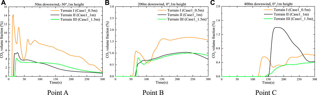
FIGURE 9. CO₂ concentrations at different locations based on the distance from the center of the CO₂ release source.

FIGURE 10

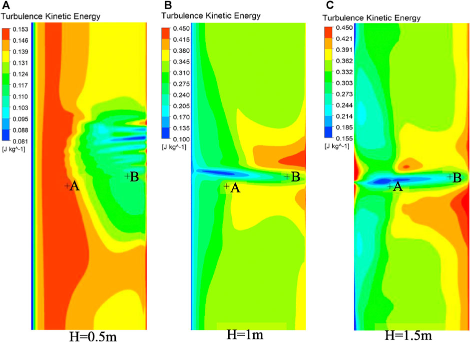
FIGURE 10. Contours of the turbulent kinetic energy at three different heights.

Figures 11, 12 demonstrate these CD-4s at different times when heights of the shrub are 0.5 and 1.5 m, respectively. Comparing with those in Figure 6, it is observed that in the initial release stage for the three height shrubs, the higher height gives rise to less degree of cloud collapse. The higher the shrub height is, the greater the thickness of the porous medium area is, and therefore, the flow field varies more obviously. Especially with the dispersion time goes on, the change is more significant. Clearly, the variation in the flow field became more remarkable (Figure 12B) at 40 s with a shrub height of 1.5 m. The CD-4 appeared as two vortex-like shapes located far from the release source. The coverage area of the isosurface also increased (Table 6). It is found by comparison that a greater shrub height led to more intense turbulent field changes in the porous medium area and more evident lateral dispersion. Generally, shrub height affects the range of cloud and the feature of CO₂ dispersion to a certain extent. Higher shrub height contributes to more complicated and noteworthy variations in the flow field, effectively delaying heavy gas dispersion and increasing lateral consequence distance.

FIGURE 11

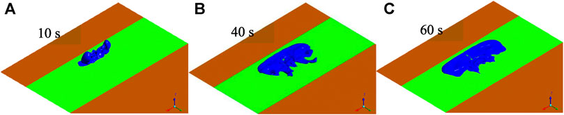
FIGURE 11. CD-4 at different time points with 0.5-m high shrubs.

FIGURE 12

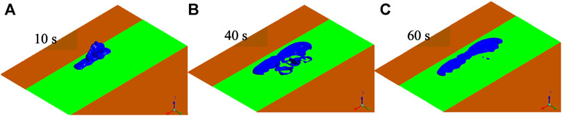
FIGURE 12. CD-4 at different time points with 1.5-m high shrubs.

TABLE 6

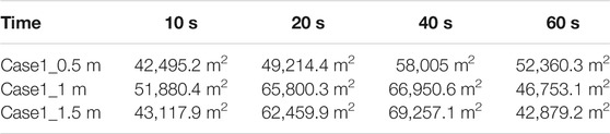
TABLE 6. Comparison of the CD-4 at different time points with shrubs of three different heights.

Effect of Shrub Porosity on Heavy Gas Dispersion

The aforementioned contents mainly have focused on the assessment of the impact of shrub region relative position and shrub height on CO₂ dispersion. However, different shrub species have different densities of branches and leaves, and also the seasons will affect these densities remarkably as well. Canopy density expressed as the porosity brings about significant variations in canopy turbulence. Therefore, it is of the great significance of investigating the effect of shrub porosity on the character of CO₂ dispersion. Nevertheless, there has a little discussion about the basic characteristics of this issue. In a sparse shrub canopy, the sparser branches and leaves result in higher porosity. As a result, the wind-blocking effect is weaker. As such, sparse canopies primarily cause variations in turbulence at the spatial level. Figure 13 compares curves of CO₂ concentration vs. time between different porosities at the three monitoring points at 1 m altitudes. The locations of the three monitoring points A, B, and C are shown in Figure 3. At point A, which located closer to the release source, time-varying concentration trends for three porosities are very similar. However, when the porosity is 0.3, the maximum CO₂ concentration is slightly higher than those in the other two cases. As the distance from the release source increased (i.e., point B in Figure 13B), the influence of porosity on the maximum gas concentration also increased. When the porosity is 0.9, the maximum CO₂ concentration at point B is significantly less than that with porosities of 0.3 and 0.6. In terms of point C located even farther away, it is observed that the gas concentration curve of porosity 0.9 increased significantly, and the maximum CO₂ concentration is more than three times higher than that of the gas concentration with the porosities of 0.3 and 0.6. The reason for this is that the gas release rate is relatively high in the initial jet state of the release, and point A is located near the release source, so the change in the porosity of the shrub had little effect on the wind speed at this point. With the continuous increase in the dispersion distance, the porous medium region has obvious differences in the wind field under different porosities. When the porosity is 0.9, the barrier effect on the wind is smaller, so it can be farther away from the release source and CO₂ is captured with a higher concentration value. For the porous medium regions with porosities of 0.3 and 0.6, when the height of the shrub is 1 m, the effect of resistance on wind filed is similar.

FIGURE 13

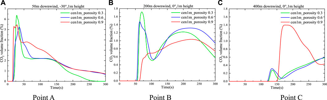
FIGURE 13. Variation of CO₂ concentration with time at three monitoring points with the same shrub height and different porosity values.

Conclusion

This article developed a CFD model to explore the influence of the shrub region on the dispersion of CO₂ released from the ruptured high-pressure pipelines. Herein, shrubs were treated as a kind of porous media, and additional momentum source terms and turbulence source terms were applied to the entire porous medium area via UDF. The CFD model was validated using previous research and existing data.

The following conclusions are drawn:

1. Shrubs as porous media have a greater impact on the near-surface flow field than shrub-free terrains. As such, shrubs are more likely to produce mechanical turbulence. The lateral dispersion is of significance, and the gas dispersion time is prolonged. Compared with the shrub-free terrain, the CD-4 of the three shrub terrains at 60 s increased by 8.1 times, 6.7 times, and 9.1 times, respectively.

2. The relative position of the shrubbery and release source impact the surface flow field of the release source significantly. When shrubs cover the release source, at the initial stage of release and owing to the increased barrier effect of shrubs on the wind, the CO₂ gas cloud rapidly collapses. Due to the influence of the porous media on the flow field, the lateral dispersion distance increases. Specifically, at 10 s, the CD-4 of the strip shrubland without cover release source is reduced by 36.9% than that of the strip shrubland covered with the release source; while compared with the strip shrubland covered with the release source, the CD-4 of the terrain of the full-covered shrub is reduced by 9.2%.

3. When shrubs are located close to the wind inlet, the impacts of the 1- and 1.5-m high shrubs on the near-surface flow field are similar. The CD-4 is also alike for the two situations. However, 0.5-m high shrubs impact the near-surface flow field scarcely, and their ability to delay gas dispersion is much lower than that of taller shrubs. The height of shrubs does not correlate linearly with delays in gas dispersion.

4. Although porosity substantially affects the resistance of shrubs to the wind, they have different effects on various terrains. When the porosity of 1-m high shrubbery ranges between 0.3 and 0.6, its impact on the flow field near the ground and the degree of gas dispersion are similar. When the porosity reaches 0.9, the impact of the multi-surface flow field of shrubs is considerably reduced, the blocking effect on the wind is weaker, and the CO₂ spreads faster.

This work supplements effective basis for understanding CO₂ dispersion over complex terrain. It also helps determine a sufficient protective distance for personnel working in resource mining and environmentally sensitive areas. Emergency plans developed based on this research can provide a reliable method for CCS-related risk assessment.

Data Availability Statement

The original contributions presented in the study are included in the article/Supplementary Material, further inquiries can be directed to the corresponding author.

Author Contributions

HW conducted experimental verification and CFD numerical simulation, analyzed the data, and wrote the manuscript. YZ made a significant contribution to the analysis and preparation of the manuscript, and he also reviewed and edited. MF helped the analysis through constructive discussions, and he also reviewed and edited. LB helped the analysis through constructive discussions. HP contributed to the research idea.

Funding

Natural Science Foundation of Hebei Province (E2019210036); Natural Science Foundation of Hebei Province (E2014210060); Fundamental research found for Hebei Province administrated Universities (ZCT202002).

Conflict of Interest

The authors declare that the research was conducted in the absence of any commercial or financial relationships that could be construed as a potential conflict of interest.

References

Ahmed, I., Bengherbia, T., Zhvansky, R., Ferrara, G., Wen, J. X., and Stocks, N. G. (2016). Validation of Geometry Modelling Approaches for Offshore Gas Dispersion Simulations. J. Loss Prev. Process Industries 44, 594–600. doi:10.1016/j.jlp.2016.07.009

CrossRef Full Text | Google Scholar

AIJ (2020). AIJ Japanese Architectural Society (AIJ) Wind Tunnel Test and Field Measurement Data. Available at: https://www.aij.or.jp.jpn/publish/cfdguide/index_e.htm (Accessed February 15, 2020).

Google Scholar

ANSYS (2011a). ANSYS FLUENT Theory Guide. USA: ANSYS Inc.

ANSYS (2011b). ANSYS FLUENT UDF Manual. USA: ANSYS Inc.

Barbano, F., Di Sabatino, S., Stoll, R., and Pardyjak, E. R. (2020). A Numerical Study of the Impact of Vegetation on Mean and Turbulence fields in a European-city Neighbourhood. Building Environ. 186. doi:10.1016/j.buildenv.2020.107293

CrossRef Full Text | Google Scholar

Bijad, E., Delavar, M. A., and Sedighi, K. (2016). CFD Simulation of Effects of Dimension Changes of Buildings on Pollution Dispersion in the Built Environment. Alexandria Eng. J. 55, 3135–3144. doi:10.1016/j.aej.2016.08.024

CrossRef Full Text | Google Scholar

Buccolieri, R., Gromke, C., Di Sabatino, S., and Ruck, B. (2009). Aerodynamic Effects of Trees on Pollutant Concentration in Street Canyons. Sci. Total Environ. 407, 5247–5256. doi:10.1016/j.scitotenv.2009.06.016

PubMed Abstract | CrossRef Full Text | Google Scholar

Buccolieri, R., Jeanjean, A. P. R., Gatto, E., and Leigh, R. J. (2018). The Impact of Trees on Street Ventilation, NOx and PM2.5 Concentrations across Heights in Marylebone Rd Street canyon. Cent. Lond. Sustain. Cities Soc. 41, 227–241. doi:10.1016/j.scs.2018.05.030

CrossRef Full Text | Google Scholar

Chen, J., Viatte, C., Hedelius, J. K., Jones, T., Franklin, J. E., Parker, H., et al. (2016). Differential Column Measurements Using Compact Solar-Tracking Spectrometers Atmos. Chem. Phys. 16, 8479–8498. doi:10.5194/acp-16-8479-2016

CrossRef Full Text | Google Scholar

COST Action 732 (2007a). Background and Justification Document to Support the Model Evaluation Guidance and Protocol. Meteorological Inst.

COST Action 732 (2007b). Best Practise Guideline for the CFD Simulation of Flows in the Urban Environment. Meteorological Inst.

COST Action 732 (2007c). Model Evaluation Cuidance and Protocol Document. Meteorological Inst.

COST Action 732 (2010). Model Evaluation Case Studies: Approach and Result. Meteorological Inst.

Ding, L., Mao, X., Yang, L., Yan, B., Wang, J., and Zhang, L. (2020). Effects of Installation Position of Fin-Shaped Rods on Wind-Induced Vibration and Energy Harvesting of Aeroelastic Energy Converter. Smart Mater. Structures 30. doi:10.1088/1361-665X/abd42b

CrossRef Full Text | Google Scholar

Dong, Z., Luo, W., Qian, G., and Lu, P. (2008). Wind Tunnel Simulation of the Three-Dimensional Airflow Patterns Around Shrubs. J. Geophys. Res. 113. doi:10.1029/2007jf000880

CrossRef Full Text | Google Scholar

Efthimiou, G. C., Andronopoulos, S., Tavares, R., and Bartzis, J. G. (2017). CFD-RANS Prediction of the Dispersion of a Hazardous Airborne Material Released during a Real Accident in an Industrial Environment. J. Loss Prev. Process Industries 46, 23–36. doi:10.1016/j.jlp.2017.01.015

CrossRef Full Text | Google Scholar

Fabbri, L., Binda, M., and Bruin, Y. Bd. (2017). Accident Damage Analysis Module (ADAM) – Technical Guidance. Luxembourg, EUR 28732 EN: Publications Office of the European Union. doi:10.2760/719457

CrossRef Full Text

Fabbri, L., and Wood, M. H. (2019). Accident Damage Analysis Module (ADAM): Novel European Commission Tool for Consequence Assessment—Scientific Evaluation of Performance. Process Saf. Environ. Prot. 129, 249–263. doi:10.1016/j.psep.2019.07.007

CrossRef Full Text | Google Scholar

Fabbri, L., Wood, M. H., Azzini, I., and Rosati, R. (2020). Global Sensitivity Analysis of the ADAM Dispersion Module: Jack Rabbit II Test Case. Atmos. Environ. 240, 117586. doi:10.1016/j.atmosenv.2020.117586

CrossRef Full Text | Google Scholar

Gale, J., and Davison, J. (2004). Transmission of CO2—safety and Economic Considerations. Energy 29, 1319–1328. doi:10.1016/j.energy.2004.03.090

CrossRef Full Text | Google Scholar

Gallagher, J., Baldauf, R., Fuller, C. H., Kumar, P., Gill, L. W., and McNabola, A. (2015). Passive Methods for Improving Air Quality in the Built Environment: A Review of Porous and Solid Barriers. Atmos. Environ. 120, 61–70. doi:10.1016/j.atmosenv.2015.08.075

CrossRef Full Text | Google Scholar

Gant, S., Weil, J., Delle Monache, L., McKenna, B., Garcia, M. M., Tickle, G., et al. (2018). Dense Gas Dispersion Model Development and Testing for the Jack Rabbit II Phase 1 Chlorine Release Experiments. Atmos. Environ. 192, 218–240. doi:10.1016/j.atmosenv.2018.08.009

CrossRef Full Text | Google Scholar

Gant, S., Tickle, G., Kelsey, A., and Tucker, H. (2021). DRIFT Dispersion Model Predictions for the Jack Rabbit II Model Inter-comparison Exercise. Atmos. Environ. 244, 117717. doi:10.1016/j.atmosenv.2020.117717

CrossRef Full Text | Google Scholar

Gavelli, F., Bullister, E., and Kytomaa, H. (2008). Application of CFD (Fluent) to LNG Spills into Geometrically Complex Environments. J. Hazard. Mater. 159, 158–168. doi:10.1016/j.jhazmat.2008.02.037

PubMed Abstract | CrossRef Full Text | Google Scholar

Götmark, F., Götmark, E., and Jensen, A. M. (2016). Why Be a Shrub? A Basic Model and Hypotheses for the Adaptive Values of a Common Growth Form. Front. Plant Sci. 7, 1–14. doi:10.3389/fpls.2016.01095

PubMed Abstract | CrossRef Full Text | Google Scholar

Gromke, C., Jamarkattel, N., and Ruck, B. (2016). Influence of Roadside Hedgerows on Air Quality in Urban Street Canyons. Atmos. Environ. 139, 75–86. doi:10.1016/j.atmosenv.2016.05.014

CrossRef Full Text | Google Scholar

Hagishima, A., Narita, K-i., and Tanimoto, J. (2007). Field experiment on Transpiration from Isolated Urban Plants. Hydrological Process. 21, 1217–1222. doi:10.1002/hyp.6681

CrossRef Full Text | Google Scholar

Havens, J., and Spicer, T. O. (1990). “LNG Vapor Dispersion Prediction with the DEGADIS Dense Gas Dispersion Model,” Report GRI 89/0242 (United States: Gas Research Institute (GRI)).

Google Scholar

Hefny Salim, M., Heinke Schlünzen, K., and Grawe, D. (2015). Including Trees in the Numerical Simulations of the Wind Flow in Urban Areas: Should We Care? J. Wind Eng. Ind. Aerodynamics 144, 84–95. doi:10.1016/j.jweia.2015.05.004

CrossRef Full Text | Google Scholar

Hong, B., Qin, H., and Lin, B. (2018). Prediction of Wind Environment and Indoor/Outdoor Relationships for PM2.5 in Different Building–Tree Grouping Patterns. Atmosphere 9, 1–39. doi:10.3390/atmos9020039

CrossRef Full Text | Google Scholar

Hsieh, K-J., Lien, F-S., and Yee, E. (2013). Dense Gas Dispersion Modeling of CO2 Released from Carbon Capture and Storage Infrastructure into a Complex Environment. Int. J. Greenhouse Gas Control. 17, 127–139. doi:10.1016/j.ijggc.2013.05.003

CrossRef Full Text | Google Scholar

IEA (2018). World Energy Outlook 2018. Paris: IEAAvailable at: https://www.iea.org/reports/world-energy-outlook-2018.

Jeanjean, A. P. R., Buccolieri, R., Eddy, J., Monks, P. S., and Leigh, R. J. (2017). Air Quality Affected by Trees in Real Street Canyons: The Case of Marylebone Neighbourhood in central London Urban Forestry & Urban Green. 22, 41–53. doi:10.1016/j.ufug.2017.01.009

CrossRef Full Text | Google Scholar

Kukkonen, J., Nikmo, J., and Riikonen, K. (2017). An Improved Version of the Consequence Analysis Model for Chemical Emergencies. ESCAPE Atmos. Environ. 150, 198–209. doi:10.1016/j.atmosenv.2016.11.050

CrossRef Full Text | Google Scholar

Kumar, P., Feiz, A-A., Ngae, P., Singh, S. K., and Issartel, J-P. (2015). CFD Simulation of Short-Range Plume Dispersion from a point Release in an Urban like Environment. Atmos. Environ. 122, 645–656. doi:10.1016/j.atmosenv.2015.10.027

CrossRef Full Text | Google Scholar

Launder, B. E., and Spalding, D. B. (1972). Lectures in Mathematical Models of Turbulence. (Waltham: Academic Press).

Li, X-B., Lu, Q-C., Lu, S-J., He, H-D., Peng, Z-R., Gao, Y., et al. (2016). The Impacts of Roadside Vegetation Barriers on the Dispersion of Gaseous Traffic Pollution in Urban Street Canyons Urban. For. Urban Green. 17, 80–91. doi:10.1016/j.ufug.2016.03.006

CrossRef Full Text | Google Scholar

Liang, L., Xiaofeng, L., Borong, L., and Yingxin, Z. (2006). Simulation of Canopy Flows Using K-ε Two-Equation Turbulence Model Withsource/sink Terms. Tsinghua Univ. (Sci. Tech.) 46, 753–756. doi:10.16511/j.cnki.qhdxxb.2006.06.001

CrossRef Full Text | Google Scholar

Lipponen, J., Burnard, K., Beck, B., Gale, J., and Pegler, B. (2011). The IEA CCS Technology Roadmap. One Year Energ. Proced. 4, 5752–5761. doi:10.1016/j.egypro.2011.02.571

CrossRef Full Text | Google Scholar

Liu, B., Liu, X., Lu, C., Godbole, A., Michal, G., and Tieu, A. K. (2016). Computational Fluid Dynamics Simulation of Carbon Dioxide Dispersion in a Complex Environment. J. Loss Prev. Process Industries 40, 419–432. doi:10.1016/j.jlp.2016.01.017

CrossRef Full Text | Google Scholar

Liu, J., Zhang, X., Niu, J., and Tse, K. T. (2019a). Pedestrian-level Wind and Gust Around Buildings with a ‘lift-Up’ Design: Assessment of Influence from Surrounding Buildings by Adopting LES. Building Simulation 12, 1107–1118. doi:10.1007/s12273-019-0541-5

CrossRef Full Text | Google Scholar

Liu, X., Godbole, A., Lu, C., and Michal, G. (2017). Investigation of Terrain Effects on the Consequence Distance of CO 2 Released from High-Pressure Pipelines. Int. J. Greenhouse Gas Control. 66, 264–275. doi:10.1016/j.ijggc.2017.10.009

CrossRef Full Text | Google Scholar

Liu, X., Godbole, A., Lu, C., Michal, G., and Linton, V. (2019b). Investigation of the Consequence of High-Pressure CO2 Pipeline Failure through Experimental and Numerical Studies. Appl. Energ. 250, 32–47. doi:10.1016/j.apenergy.2019.05.017

CrossRef Full Text | Google Scholar

Liu, X., Godbole, A., Lu, C., Michal, G., and Venton, P. (2015). Optimisation of Dispersion Parameters of Gaussian Plume Model for CO(2) Dispersion. Environ. Sci. Pollut. Res. Int. 22, 18288–18299. doi:10.1007/s11356-015-5404-8

PubMed Abstract | CrossRef Full Text | Google Scholar

Liu, Z., Zhou, Y., Huang, P., Sun, R., Wang, S., and Ma, X. (2012). Scaled Field Test for CO2 Leakage and Dispersion from Pipelines. J. Chem. Ind. Eng. (China) 63, 1651–1659. doi:10.3969/j.issn.0438-1157.2012.05.046

CrossRef Full Text | Google Scholar

Luketa-Hanlin, A., Koopman, R. P., and Ermak, D. L. (2007). On the Application of Computational Fluid Dynamics Codes for Liquefied Natural Gas Dispersion. J. Hazard. Mater. 140, 504–517. doi:10.1016/j.jhazmat.2006.10.023

PubMed Abstract | CrossRef Full Text | Google Scholar

Mazzoldi, A., Hill, T., and Colls, J. J. (2008). CFD and Gaussian Atmospheric Dispersion Models: A Comparison for Leak from Carbon Dioxide Transportation and Storage Facilities. Atmos. Environ. 42, 8046–8054. doi:10.1016/j.atmosenv.2008.06.038

CrossRef Full Text | Google Scholar

Meroney, R. N. (2010). CFD Prediction of Dense Gas Clouds Spreading in a Mock Urban Environment, 5th International Symposium on Computational Wind Engineering (CWE2010). North Carolina, USA: Chapel Hill.

Metz, B., Davidson, O., de Coninck, H., Loos, M., and Meyer, L. (2005). IPCC Special Report on Carbon Dioxide Capture and Storage United States. Available at https://www.osti.gov/biblio/20740954

Mochida, A., Tabata, Y., Iwata, T., and Yoshino, H. (2008). Examining Tree Canopy Models for CFD Prediction of Wind Environment at Pedestrian Level. J. Wind Eng. Ind. Aerodynamics 96, 1667–1677. doi:10.1016/j.jweia.2008.02.055

CrossRef Full Text | Google Scholar

Moonen, P., Gromke, C., and Dorer, V. (2013). Performance Assessment of Large Eddy Simulation (LES) for Modeling Dispersion in an Urban Street canyon with Tree Planting. Atmos. Environ. 75, 66–76. doi:10.1016/j.atmosenv.2013.04.016

CrossRef Full Text | Google Scholar

Morales, A. I. G. C., Olano Mendoza, J. M., Eugenio Gozalbo, M., and Camarero Martínez, J. J. (2012). Arboreal and Prostrate Conifers Coexisting in Mediterranean High Mountains Differ in Their Climatic Responses. Dendrochronologia 30, 279–286. doi:10.1016/j.dendro.2012.02.004

CrossRef Full Text | Google Scholar

Myers-Smith, I. H., Elmendorf, S. C., Beck, P. S. A., Wilmking, M., Hallinger, M., Blok, D., et al. (2015). Climate Sensitivity of Shrub Growth across the Tundra Biome. Nat. Clim. Change 5, 887–891. doi:10.1038/nclimate2697

CrossRef Full Text | Google Scholar

NIOSH (2005). NIOSH Pocket Guide to Chemical Hazards, DHHS (NIOSH) Publicatior No. 2005-149 (Columbia Parkway: NIOSH Publications). Available at https://www.cdc.gov/niosh/docs/2005-149/pdfs/2005-149.pdf

NOAA/EPA (1992). ALOHA User's Manual and Theoretical Description. Reports available from: NOAA/HMRAD, 7600 Sand Point Way NE, Seattle, WA 98115 and on CAMEO/ALOHA web site.

Google Scholar

Nowak, D. J., Hirabayashi, S., Bodine, A., and Hoehn, R. (2013). Modeled PM2.5 Removal by Trees in Ten U.S. Cities and Associated Health Effects. Environ. Pollut. 178, 395–402. doi:10.1016/j.envpol.2013.03.050

PubMed Abstract | CrossRef Full Text | Google Scholar

Pellizzari, E., Camarero, J. J., Gazol, A., Granda, E., Shetti, R., Wilmking, M., et al. (2017). Diverging Shrub and Tree Growth from the Polar to the Mediterranean Biomes across the European Continent. Glob. Change Biol. 23, 3169–3180. doi:10.1111/gcb.13577

PubMed Abstract | CrossRef Full Text | Google Scholar

Peters, G. P., Andrew, R. M., Boden, T., Canadell, J. G., Ciais, P., Quere, C. L., et al. (2013). The challenge to Keep Global Warming below 2 °C. Nat. Clim. Change 3, 4–6. doi:10.1038/nclimate1783

CrossRef Full Text | Google Scholar

Peterson, E. W., and Hennessey, J. P. (1978). On the Use of Power Laws for Estimates of Wind Power Potential. J. Appl. Meteorology 17, 390–394. doi:10.1175/1520-0450(1978)017<0390:OTUOPL>2.0.CO;2

CrossRef Full Text | Google Scholar

Ryan, S. D., and Ripley, R. C. (2020). A Geometric Multigrid Treatment of Immersed Boundaries for Simulating Atmospheric Dispersion in Complex Urban Environments. Atmos. Environ. 237, 117685. doi:10.1016/j.atmosenv.2020.117685

CrossRef Full Text | Google Scholar

Sabatino, S. D., Buccolieri, R., Pappaccogli, G., and Leo, L. S. (2015). The Effects of Trees on Micrometeorology in a Real Street canyon: Consequences for Local Air Quality. Int. J. Environ. Pollut. 58, 100–111. doi:10.1504/IJEP.2015.076587

CrossRef Full Text | Google Scholar

Simpson, S. M., Miner, S., Mazzola, T., and Meris, R. (2020). HPAC Model Studies of Selected Jack Rabbit II (JRII) Releases and Comparisons to Test Data. Atmos. Environ. 243, 117675. doi:10.1016/j.atmosenv.2020.117675

CrossRef Full Text | Google Scholar

Sklavounos, S., and Rigas, F. (2006). Simulation of Coyote Series Trials—Part I:: CFD Estimation of Non-isothermal LNG Releases and Comparison with Box-Model Predictions. Chem. Eng. Sci. 61, 1434–1443. doi:10.1016/j.ces.2005.08.042

CrossRef Full Text | Google Scholar

Smagorinsky, J. (1963). GENERAL CIRCULATION EXPERIMENTS WITH THE PRIMITIVE EQUATIONS: I. THE BASIC EXPERIMENT*. Monthly Weather Rev. 91, 99–164. doi:10.1175/1520-0493(1963)091<0099:GCEWTP>2.3.CO;2

CrossRef Full Text | Google Scholar

Stabile, L., Arpino, F., Buonanno, G., Russi, A., and Frattolillo, A. (2015). A Simplified Benchmark of Ultrafine Particle Dispersion in Idealized Urban Street Canyons: A Wind Tunnel Study. Building Environ. 93, 186–198. doi:10.1016/j.buildenv.2015.05.045

CrossRef Full Text | Google Scholar

Takano, Y., and Moonen, P. (2013). On the Influence of Roof Shape on Flow and Dispersion in an Urban Street canyon. J. Wind Eng. Ind. Aerodynamics 123, 107–120. doi:10.1016/j.jweia.2013.10.006

CrossRef Full Text | Google Scholar

Tan, W., Wang, K., Li, C., Liu, L., Wang, Y., and Zhu, G. (2018). Experimental and Numerical Study on the Dispersion of Heavy Gases in Urban Environments. Process Saf. Environ. Prot. 116, 640–653. doi:10.1016/j.psep.2018.03.027

CrossRef Full Text | Google Scholar

Tauseef, S. M., Rashtchian, D., and Abbasi, S. A. (2011). CFD-based Simulation of Dense Gas Dispersion in Presence of Obstacles. J. Loss Prev. Process Industries 24, 371–376. doi:10.1016/j.jlp.2011.01.014

CrossRef Full Text | Google Scholar

Toja-Silva, F., Chen, J., Hachinger, S., and Hase, F. (2017). CFD Simulation of CO2 Dispersion from Urban thermal Power Plant: Analysis of Turbulent Schmidt Number and Comparison with Gaussian Plume Model and Measurements. J. Wind Eng. Ind. Aerodynamics 169, 177–193. doi:10.1016/j.jweia.2017.07.015

CrossRef Full Text | Google Scholar

Tominaga, Y., and Stathopoulos, T. (2010). Numerical Simulation of Dispersion Around an Isolated Cubic Building: Model Evaluation of RANS and LES. Building Environ. 45, 2231–2239. doi:10.1016/j.buildenv.2010.04.004

CrossRef Full Text | Google Scholar

Vos, P. E. J., Maiheu, B., Vankerkom, J., and Janssen, S. (2013). Improving Local Air Quality in Cities: To Tree or Not to Tree? Environ. Pollut. 183, 113–122. doi:10.1016/j.envpol.2012.10.021

PubMed Abstract | CrossRef Full Text | Google Scholar

Wang, H., Liu, B., Liu, X., Lu, C., Deng, J., and You, Z. (2021a). Dispersion of Carbon Dioxide Released from Buried High-Pressure Pipeline over Complex Terrain. Environ. Sci. Pollut. Res. 28, 1–14. doi:10.1007/s11356-020-11012-7

CrossRef Full Text | Google Scholar

Wang, J., Sun, S., Tang, L., Hu, G., and Liang, J. (2021b). On the Use of Metasurface for Vortex-Induced Vibration Suppression or Energy Harvesting. Energ. Convers. Manage. 235, 113991. doi:10.1016/j.enconman.2021.113991

CrossRef Full Text | Google Scholar

Wingstedt, E. M. M., Osnes, A. N., Åkervik, E., Eriksson, D., and Reif, B. A. P. (2017). Large-eddy Simulation of Dense Gas Dispersion over a Simplified Urban Area. Atmos. Environ. 152, 605–616. doi:10.1016/j.atmosenv.2016.12.039

CrossRef Full Text | Google Scholar

Wu, X., Zou, X., Zhou, N., Zhang, C., and Shi, S. (2015). Deceleration Efficiencies of Shrub Windbreaks in a Wind Tunnel. Aeolian Res. 16, 11–23. doi:10.1016/j.aeolia.2014.10.004

CrossRef Full Text | Google Scholar

Zhang, C. (2009). “Study on the Assessment and Remote Sensing Classification Technique of Shrub in Tibet,”. Doctoral dissertation.

Google Scholar