Forecast Quality of Physics-Based and Data-Driven PV Performance Models for a Small-Scale PV System

In the context of smart grids, the need for forecasts of the power output of small-scale photovoltaic (PV) arrays increases as control processes such as the management of flexibilities in the distribution grid gain importance. However, there is often only very little knowledge about the PV systems installed: even fundamental system parameters such as panel orientation, the number of panels and their type, or time series data of past PV system performance are usually unknown to the grid operator. In the past, only forecasting models that attempted to account for cause-and-effect chains existed; nowadays, also data-driven methods that attempt to recognize patterns in past behavior are available. Choosing between physics-based or data-driven forecast methods requires knowledge about the typical forecast quality as well as the requirements that each approach entails. In this contribution, the achieved forecast quality for a typical scenario (day-ahead, based on numerical weather predictions [NWP]) is evaluated for one physics-based as well as five different data-driven forecast methods for a year at the same site in south-western Germany. Namely, feed-forward neural networks (FFNN), long short-term memory (LSTM) networks, random forest, bagging and boosting are investigated. Additionally, the forecast quality of the weather forecast is analyzed for key quantities. All evaluated PV forecast methods showed comparable performance; based on concise descriptions of the forecast approaches, advantages and disadvantages of each are discussed. The approaches are viable even though the forecasts regularly differ significantly from the observed behavior; the residual analysis performed offers a qualitative insight into the achievable forecast quality in a typical real-world scenario.

1. Introduction

Applications for forecasting the power produced by photovoltaic (PV) systems include the prediction of possible overload situations in the grid and the planning of corresponding countermeasures such as flexibility management, as well as the local optimization of energy consumption in a nanogrid.

With an increasing percentage of houses that feature small-size PV systems and the possibility of local (own) consumption, the need for reliable power forecasts to be used in subsequent processes also increases: Kraiczy et al. (2019) outline applications of PV forecasting in distribution system operation and list requirements that these would entail. The authors expect an increasing demand for PV forecasts and list day-ahead forecasts for congestion management as one of the major use cases. However, they also acknowledge that the lack of information about installed systems is a dominant characteristic for small-scale PV systems at the distribution level, which, in sum, provide far more power than large-scale PV systems that are required to provide information (Kraiczy et al., 2019, section 3).

Roughly speaking, there are two approaches to creating models of PV systems: physics-based methods attempt to model the system's behavior by physical equations and causal relations, whereas data-driven methods attempt to identify patterns in meteorological and power output data to create predictions. Hybrid methods that attempt to combine the advantages of physics-based and data-driven methods exist, as well (for example Massucco et al., 2019).

Physics-based PV performance models can be parameterized by a small set of quantities that exist in the real world and can thus be measured or taken from data sheets. Typically, a model is valid for a whole class of similar systems—a parameter set defines a specific model instance, but the underlying system of equations (the model) stays the same. Consequently, no power measurements are necessary to create forecasts for a new site. This means that this approach can be scaled to provide forecasts for many systems rapidly, and that forecasts for systems that do not exist in reality (yet) can also be created.

On the other hand, data-driven approaches such as neural networks require large amounts of historical power output data as well as historical weather forecasts. Obtaining such data often proves to be difficult for both technical as well as organizational reasons, for example concerns about the protection of privacy rights. However, forecast models can be created without knowledge about the system's technical details as long as the plausibility of results can be assessed.

Both approaches rely on weather forecasts as an input to the model. Typically, the irradiance in the horizontal plane and the air temperature are required inputs. Possibly, forecasts for wind speed, cloud cover, snow, and other quantities could also be required.

In this paper, the question “how do physics-based/data-driven PV system performance modeling approaches compare in a typical real-life scenario?” is answered by comparing one physics-based PV performance model and several data-driven forecast methods with respect to their performance, but also additional criteria such as the prerequisites for their usage. By “typical real-life scenario,” we wish to summarize the context: day-ahead forecasts based on numerical weather prediction (NWP) forecasts with only little knowledge about the PV system itself.

Similar work is, for example, reported by Ogliari et al. (2017), Richter et al. (2015, section 3.2). Ogliari et al. (2017) compared a hybrid model based on artificial neural networks to a three-parameter diode model by using the power measurements of a single PV module (245 Wp) and weather forecasts provided at 11 a.m. on the previous day and also investigated the effects of different amounts of training data and different training methods on the results. Their analysis is predominantly based on the normalized mean absolute error (nMAE).

In contrast, the comparison presented in this paper is based on an analysis of the day-ahead forecast performance for an 82 kWp-PV system installed in south-western Germany for the entire year 2019 using the weather forecasts created at 9 p.m. UTC for the following day. The analysis follows best practices suggested in the literature and comprises qualitative and quantitative assessments based on residual analysis and selected error metrics, as described in section 2.

The models for which the forecast quality is evaluated are described in section 3. Since the uncertainty of the weather forecast represents a major source of error (Richter et al., 2015, section 6), an analysis of the achieved forecast quality at a nearby weather station for key quantities is included in section 4.1. The primary use of the results of the performance analysis, shown in section 4.2, is the ability to quantify the uncertainty of a forecast as described in section 5.1. The conclusions drawn from the analysis are stated in section 5.2.

2. Method

There are many sources of uncertainty both when creating PV forecasts as well as when analyzing the forecast's quality by comparison to measurement data. In their review of these uncertainties, Richter et al. (2015) identify three groups: uncertainties with respect to the measurement or estimation of the solar resource, uncertainties in PV modeling, and other “field-related uncertainties.” They express the individual uncertainties in terms of the normalized root mean square error (nRMSE) and calculate the overall uncertainty by means of error propagation. When “using state-of-the-art models”(Richter et al., 2015, section 4) to calculate the generated energy, the authors arrive at an estimated uncertainty of ±6–±8%.

Despite this number can be useful for planning, operations, and management of PV systems, a more detailed analysis is required when attempting to understand and compare the characteristics of different forecast methods. Furthermore, Dobreva et al. (2020, p. 135) point out that the RMSE is sensitive to outliers, scale-dependent unless normalized, and lacking a “criterion indicating whether the deviation of the model is unacceptably large or reasonably small.”

In this section, the overall process for evaluating the forecast performance of the use case under investigation is outlined by explaining the graphical residual analysis applied, summarizing the metrics used, stating the equations for applying the gained information to add uncertainty information to a newly created forecast, and describing the data sets upon which the analysis was performed.

2.1. Performance Evaluation

At the start of the analysis, PV performance forecasts, boundary conditions, measurement values, and residuals (“forecast minus measurement”) were saved in a time series database (TSDB) for the entire time frame under investigation.

Then, different analyses were performed as suggested by Stein et al. (2010) as a “standardized approach to PV system performance model validation.” Stein et al. (2010) focused on the use of their approach for model validation and improvement, and thus stated that environment conditions measured as accurately as possible should be used as model input. However, subsequent processes “see” the overall forecast including the uncertainty of the weather forecast, therefore the suggested analyses were applied to the overall forecast as well.

First, measurements, forecasts, residuals, and characteristic values per day were plotted over time to allow for an interactive exploration of the data set and to identify possible (seasonal) trends or sudden changes. Best, worst and average forecast performances per day were identified to show and characterize the range of achieved forecast quality. Three days in winter were removed from the analysis because the system was obviously covered in snow; throughout the year, there are 11 more days that were removed from the analysis because there was no weather data for technical reasons.

Then, scatter plots of forecast and measurement over measured quantities were created. These plots indicate the forecast's variance, show outliers in the data set, and could also indicate systematic errors such as consistent forecast errors due to panel aging or shadowing.

For a good model that describes the relevant aspects of a system with the necessary accuracy and without any systematical errors, the residuals are expected to follow a normal distribution (page 3 in Stein et al., 2010; Dobreva et al., 2020, section 2.1). Therefore, a normal distribution with the same standard deviation σ as the residuals and an expected value μ of zero was plotted on top of a histogram of the residuals as a form of normality test. For proper scaling, a whole-number fraction of the standard deviation was chosen as bin size for the histogram and the probability density function of the normal distribution was multiplied by a scaling factor as shown in Equation (1), where N_s represents the total number of residuals, and n_b/σ denotes the number of bins per standard deviation.

$\begin{array}{ll}\text{PDF}=\frac{\sigma N_s}{n_{b/\sigma }}\times \frac{1}{\sigma \sqrt{2\pi }}{e}^{-\frac{1}{2}{\left(\frac{x-\mu }{\sigma }\right)}^2}& (1)\end{array}$

In addition to the qualitative insight that the residual analysis provides, a quantitative metric to assess the overall performance in terms of a number that allows ranking of different models is desirable. Ideally, this metric should be scale independent and robust, allow the comparison of different models at the same site and at different sites, and accurately represent the quality of the forecast.

The metrics s (Equation 2) and mm (Equation 3) proposed by Dobreva et al. (2020) fulfill these requirements and are consequently used in this work. In the defining equations, P_i represents the set of predicted values and M_i the corresponding measurements; r denotes the Pearson correlation coefficient (compare Dobreva et al., 2020, Appendix A.1).

$\begin{array}{ll}s=\sqrt{2(1-r)}& (2)\end{array}$

$\begin{array}{ll}mm=\frac{{\displaystyle {\sum }_{i=1}^n}min(P_i,M_i)}{{\displaystyle {\sum }_{i=1}^n}max(P_i,M_i)}& (3)\end{array}$

Since s emphasizes the similarity of the form of measured and forecasted values and is independent of their magnitude, mm as a metric of how well the magnitude of values is reproduced is needed as well. Table 1 summarizes the properties of s and mm.

TABLE 1

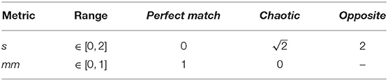
Table 1. Basic properties of the metrics s and mm.

As an example of how the proposed analysis looks like, consider the validation results of the physics-based PV-performance model described in section 3.1 against parts of the “New Data Set for Validating PV Module Performance Models” published by Marion et al. (2014): to ensure that the model equations were correctly implemented and to verify the general validity of the model, a model instance representing the HIT05667-module installed in Eugene/Oregon from December 20, 2012 through January 20, 2014 was created.

First, simulation results of this model instance using measured diffuse horizontal and direct horizontal (calculated as difference between global and diffuse) irradiance as well as ambient temperature as boundary conditions were compared to measurements for a single, perfectly sunny day (2013-05-03), as shown in Figure 1A. Measurements are shown in dark gray and the forecast in blue. For this site, the model slightly overestimates the power output in the morning and slightly underestimates the module's performance in the early morning, around noon, and in the late evening. Nonetheless, a good agreement between forecast and measurements can be achieved with only five parameters (location, azimuth and tilt angle, efficiency at reference conditions, and total area).

FIGURE 1

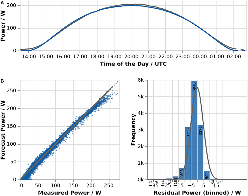
Figure 1. Comparison of measurements and the forecast created using the physics-based model for the HIT05667-module in Eugene/Oregon by means of a run plot for May 5, 2013 (A) and scatter plot and histogram of residuals for three and a half months (March 15, 2013–June 25, 2013, B).

For the time period between March 15, 2013 and June 25, 2013, a scatter plot of forecast against measured values and a histogram of the residuals were created (Figure 1B). It confirms the general validity of the model as well as the slight deviations in the form of the power curve already seen in Figure 1A. About 43% of the 13,875 calculated residuals fall in the bin from −5 to 0 W; 89% of the forecast values differ from the measurement by no more than −10 to +5 W.

The metrics confirm a very good match (s = 0.07, mm = 0.95) and there are no apparent issues. It is thus concluded that the implemented model represents the power output of a PV plant accurately enough to use it for creating PV performance forecasts.

2.2. Adding Uncertainty Information to Forecasts

Visualizing a forecast over time as a single line implies exactness; the inherent uncertainty of the forecast and its confidence level(s) are not shown. Therefore, such visualizations are incomplete at best and misleading at worst, resulting in frequent misinterpretations (Toet et al., 2016).

In order to accurately convey the inherent uncertainty of a forecast and thereby increase the potential value it has to a user, the information collected on the forecast accuracy in the past was extrapolated and applied to newly created forecasts based on the assumption that the distribution of residuals in the future is similar to their distribution in the past.

This extrapolation is based on the past distribution of the relative error $e_i=\frac{P_i-M_i}{M_i}$, evaluated at each time instant i, in terms of the 25 and 75% quartiles Q₁ and Q₃. Equations (4b) and (4c) are used to calculate the extent of the confidence band for the 50% confidence level.

$\begin{array}{ll}cban{d}_{75\%,upper}=min\left[\left(\frac{1}{1+O_1}*forecast\right),P_{max}\right]& (\mathrm{4a})\end{array}$

$\begin{array}{ll}cban{d}_{50\%,upper}=min\left[\left(\frac{1}{1+Q_1}*forecast\right),P_{max}\right]& (\mathrm{4b})\end{array}$

$\begin{array}{ll}cban{d}_{50\%,lower}=max\left[\left(\frac{1}{1+Q_3}*forecast\right),0\right]& (\mathrm{4c})\end{array}$

$\begin{array}{ll}cban{d}_{75\%,lower}=max\left[\left(\frac{1}{1+O_7}*forecast\right),0\right]& (\mathrm{4d})\end{array}$

Their interpretation is as follows: 50% of the observations exhibited a relative forecast error e_i between Q₁ and Q₃. If e_i is positive, it means that the forecast overestimated the quantity; if it is negative, the quantity was underestimated. Consequently, the quantity will be greater than the forecast with the same frequency that the forecast underestimated the quantity in the past; the upper extent of the confidence band is thus defined by Q₁. Symmetrically, the quantity is expected to be smaller than the forecast with the same frequency the forecast overestimated the quantity; meaning that the lower extent of the confidence band is defined by Q₃. Combined, the quantity is expected to fall in the resulting confidence band with a likelihood of 50%. The same argument applies for the calculation of the 75% confidence level based on the 12.5 and 87.5% octiles O₁ and O₇, as shown in Equations (4a) and (4d). For obvious reasons, the confidence band is limited by the installed maximum power of the PV system at hand and 0 W, respectively.

When comparing PV performance forecasts to power measurements for several days, it can be seen that the forecast quality differs depending on the environmental conditions: forecasts tend to be best on perfectly sunny days and worst on days with highly varying conditions; absolute errors are obviously largest around noon; etc.

In order to account for this and improve the accuracy of the confidence band, it is thus desirable to cluster model performance depending on the environmental conditions with the aim of identifying conditions for which similar forecast performance was achieved. Candidate variables for clustering include angle of incidence and time of the day; clearness or clear sky indices; and more elaborate estimation schemes of irradiance variability as proposed by Schroedter-Homscheidt et al. (2018).

For this work, the instantaneous clear sky index 1 − k_c (Equation 5) based on the forecasts for global horizontal irradiance and the calculated clear sky irradiance was selected for clustering forecast performance. Reasons for this are that unlike time of the day or angle of incidence, it does not hide seasonal or daily effects; in contrast to cloud cover, it is available in the same temporal resolution as irradiance forecasts; and its calculation is much less involved than the classification scheme suggested by Schroedter-Homscheidt et al. (2018). For calculation of the clear sky irradiance irr_cs,ghi, the algorithm suggested by Ineichen and Perez (2002) in its implementation in version 0.7.2 of pvlib (Holmgren et al., 2018) was used.

$\begin{array}{ll}1-k_c=\{\begin{array}{ll}NaN& \text{if }ir{r}_{cs,ghi}<10\\ 1-\frac{ir{r}_{global}}{ir{r}_{cs,ghi}}& \text{otherwise}\end{array}& (5)\end{array}$

The value of 1 − k_c is 0 for perfectly sunny conditions and 1 for total cloud cover. Negative values for 1 − k_c are possible if clouds that are still in sunlight after the sun has sunk below the horizon increase the brightness beyond the level that would have been present had there been no clouds. In order to avoid unphysical very large negative values, 1 − k_c is set to NaN if the clear sky irradiance is below 10 W/m².

2.3. Data Sets

There were three data sets available, which enabled the analysis of the forecast quality.

First, power measurements taken in a 15-min interval of two PV plants located in Saarlouis were provided by the Saarlouis utility company. In addition to the measurement data, information about the modules used, their total number, the exact location, and their orientation and tilt angles were provided.

Second, measured climate data and the forecast runs of the COSMO-D2 numerical weather prediction model were available since February 2, 2018. Since 2017, the German National Meteorological Service (abbreviated DWD for “Deutscher Wetterdienst”) is required by law to provide most of its data as open data¹. This includes both climate data measured at many weather stations as well as the results of different forecast models. Of these forecast models, the so-called COSMO-D2 numerical weather prediction model² provides the highest temporal and spatial resolution, but also the lowest forecast horizon. Specifically, forecasts for the next 27 h with a temporal resolution of 60 min (15 min for some quantities such as irradiance; +45 h at 3 o'clock UTC) are provided every 3 h. The grid spans Germany and some neighboring areas with a spatial resolution of approximately 2.2 km.

For creating the forecasts using the physics-based PV array performance model (section 3.1), the forecasts for direct and diffuse irradiance in the horizontal plane; air temperature at 2 m above ground; and wind speed at 10 m above ground at the grid point closest to the site of interest were used. For creation of the data-driven forecasts, the proprietary SolarForecast-API provided by Meteotest³ was used instead.

3. Modeling

The PV system under investigation consists of 87 modules with a total surface area of 127 m², tilted at 17° and oriented toward east, and 268 modules tilted at 30° and oriented toward south, with a surface area of 391 m². Data sheets state an efficiency of 17% under reference conditions for both module types installed. The system is in operation since 2010 and there is no shadowing throughout the entire day.

Below, it is summarized how this system is represented using the different modeling approaches. Additionally, their requirements with regard to input data, model creation, and model instantiation are outlined.

3.1. PV Array Performance Model

The physics-based PV array performance model under investigation calculates the power trajectory over time based on direct and diffuse irradiance in the horizontal plane, air temperature and wind speed, and the sun's position relative to the system's location.

Below, the major effects taken into account and the equations used are summarized, but a full description of the model is beyond the scope of this article. Refer to the repository on GitHub⁴ for details. Note that the model does not constitute an original contribution; it is merely an implementation of existing models in the Modelica language and largely based on Jonas et al. (2018) and the description of the modeling steps provided by the Performance Modeling Collaborative (2020).

To summarize, the model calculates the power generated by the PV array as the product of the global irradiance in the plane of array (POA), the total area of the PV panels, the efficiency of the PV module under reference conditions, and a factor accounting for the varying efficiency of the conversion depending on the loss effects of incidence angle, irradiance, and PV cell temperature. The effects of DC and mismatch losses, DC/DC MPPT, snow cover, shading, and soiling or aging effects are not represented in the model. DC/AC conversion losses are accounted for by means of a constant efficiency factor.

The weather forecast only provides values for diffuse and direct irradiance in the horizontal plane. Since PV modules are typically tilted, a conversion to the plane of array is necessary. First, the angle of incidence, the angle between the surface normal and the sun beam, is calculated as a function of the sun's position relative to the system (Reda and Andreas, 2008) in terms of solar zenith angle and solar azimuth angle and the tilt and azimuth angle of the PV array. Second, direct and diffuse irradiance in the horizontal plane are converted to the plane of array. A simple geometrical formula is used for the direct irradiance, but conversion of diffuse irradiance requires a more elaborate model. In this case, the anisotropic model by Perez et al. (1987) is used, which also calculates the irradiance reflected from the ground. Finally, the global irradiance in the plane of array is the sum of direct, diffuse, and reflected irradiance.

Reflection losses, irradiance-dependent module efficiency, and temperature dependency comprise the effects accounted for by the varying efficiency factor. The reflection losses are modeled by a physical model for the incident angle modifier in the corrected version presented in Performance Modeling Collaborative (2020, section “Physical IAM Model”) and originally published by De Soto et al. (2006, section 3). The decreased efficiency of the module with lower global irradiance at 25°C is modeled as suggested by Heydenreich et al. (2008, Equation 3) and scaled to different module temperatures as suggested in the following equation in that paper, using the power temperature coefficient of the PV cells. To calculate the module temperature as a function of ambient temperature and wind speed, the model by Faiman (2008, Equation 5) is used.

The parameters necessary for calculating the overall varying efficiency factor as well as their default values⁵ are listed in Table 2.

TABLE 2

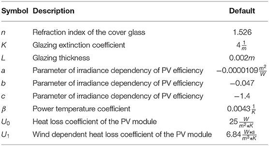
Table 2. Parameters for the calculation of the varying efficiency factor and their default values.

For analysis of the forecast quality, a model instance for both the reference module and the system of interest were instantiated using the parameters shown in Table 3 and the default values for the calculation of module efficiency are shown in Table 2. The parameter values that are not determined by the setup at the site were taken from data sheets. In the remainder of the paper, the identifier modelica is used for the physics-based parametric PV model described in this subsection.

TABLE 3

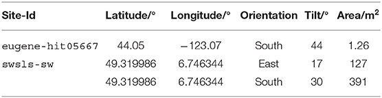
Table 3. Model parameters per site.

3.2. Data-Driven Forecast Models

Due to the non-linear and time-varying characteristics of the PV output generation, machine learning approaches like neural networks (Hossain and Mahmood, 2020) or ensemble learning techniques (Ahmad et al., 2018) such as random forest are suitable for developing models to learn and forecast the solar power generation day-ahead and intraday based on the available weather forecast data. The weather forecast features data, and the real power data are provided on a 15 min interval basis. Each plant is trained separately. The training is based on historical weather forecasts and power production measurements. The considered meteorological features are global radiation, diffuse and direct radiation, temperature, relative humidity, precipitation, and wind speed. Additionally, corresponding temporal features such as time, day, and month are also taken into account.

The dataset is roughly partitioned into 70% training set, 10% validation set, and 20% test set. Specifically, we use data from 2013 to 2018 for training and validation and data from 2019 as a test set.

Figure 2 illustrates the development process of the forecasting models based on historical weather forecasts and historical power production measurements. The process can be summarized in the following steps:

1. On the collection of the data follows a preprocessing step consisting of cleansing the data, in order to detect and clean missing data and extreme outliers in the measurements and weather forecast, to take into account the throttling time due to scheduled work on the PV plant, etc. At that stage, many strategies can be employed, for example, ignoring the extreme outliers, filling through extrapolation the gap caused by missing data, etc. Through this preliminary analysis of the raw data, the quality of the data set to be used is enhanced. The following feature engineering consists of extracting from the dataset the most relevant features that have an influence in the forecasting. The dataset is then normalized and split into training, validation, and test set.

2. Choose a model type (feed forward neural network, bagging method, etc.), specify the parameters and train and validate the defined model.

3. If the resulting model is acceptable, then evaluate with new data (test set) and save the model for future use.

4. If not, then (a) adjust the model-specific hyper-parameters, for example, number of trees, size of the feature set, etc. for the tree-based models or number of hidden layers and number of neurons per layer for the models based on neural network and (b) repeat the training and validation steps.

5. Further models can be developed with the same procedure.

FIGURE 2

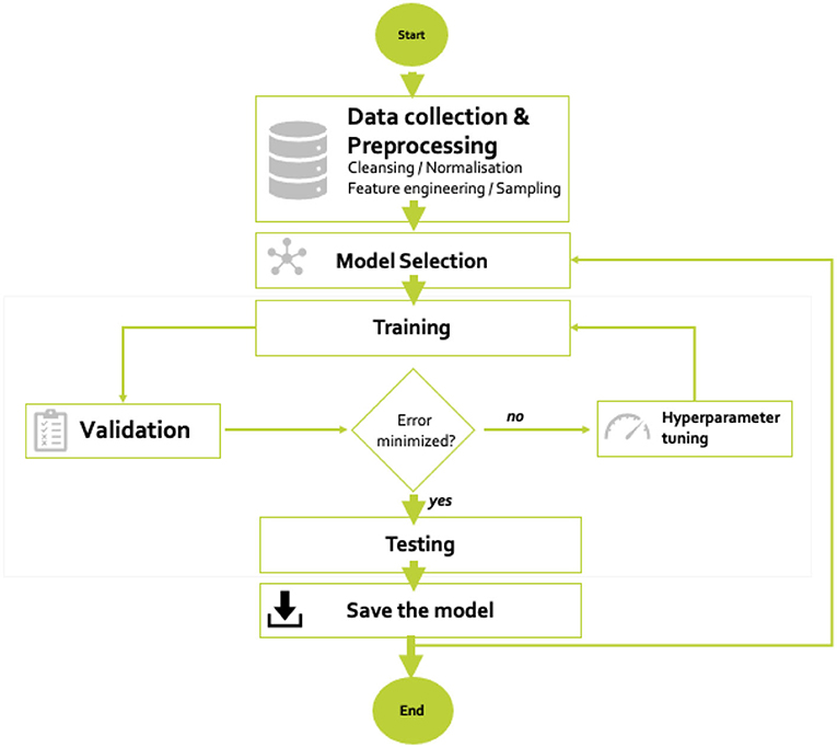
Figure 2. Flow diagram of the development process of the data-driven photovoltaic (PV) power forecasting models.

From a technical perspective, the model implementation relies on Python and the TensorFlow and scikit-learn frameworks, all of which are available under free/libre and open-source licenses.

3.2.1. Approaches Based on Neural Networks

The two first data-driven forecasting models are based on neural networks, as described as follows.

• Feed Forward Neural Networks (FFNN) (Ramsami and Oree, 2015) are characterized by unidirectional connections, from input to output. A feed-forward coupled network represents actually a directed acyclic graph. In this architecture, the neurons are organized in layers. We have being developing several models using several layers. In practice, the number of layers varies from 4 to 5, including an input layer, an output layer, and two or three hidden layers. In FFNNs, each layer is full connected with the successive layer. The input layer contains as many neurons as the size of the input space corresponding to the time elements and meteorological parameters, and the output layer contains a single neuron for the forecast value. In sum, we use two hidden layers. ReLU activation function and adam optimizer are set for the training of the network structure. To get the forecasting for the whole day, the results of the 96 quarter hours are eventually concatenated.

• Long Short-Term Memory (LSTM) (Gao et al., 2019) represent a specific kind of recurrent neural networks. They are suitable for the processing of problems where temporal aspects or sequences need to be explicitly considered, for example, in language processing.

3.2.2. Approaches Based on Ensemble Machine Learning

Ensemble machine learning refers to a supervised learning technique based on the idea that combining a large number of so-called weak learners results in much better performance than the individual performance of these weak learners, as their errors compensate each other (Ahmed Mohammed and Aung, 2016; Ahmad et al., 2018). The process consists of two steps: (1) design and training of basic learners; (2) a combination of the results of the basic learners to a single prediction by using assembling techniques such as averaging, voting, and weighted combination. When basic learners of the same type are used, the approach is referred as homogeneous ensemble model and when the basic learners are built of different algorithms, it is called heterogeneous ensemble method.

• Bagging (BAG) (Choi and Hur, 2020) regressors help to improve model performance by training in parallel each basic learner on a random subset of the training dataset and averaging the resulting single forecasts.

• Boosting (XGB [for Extreme Gradient Boosting]) is like bagging but runs sequentially. The idea behind it is that each basic learner should learn from the errors of the previous ones.

• Random Forest (RF) builds several basic learners, e.g., regression trees, by (1) training each single learner on a different random subset of the available dataset (as in bagging), (2) but also by selecting for each basic model a random combination of the features, and (3) finally aggregating them to get a more accurate and more robust result. As decision and regression tree tend to overfit, RF often yields good generalization.

We combine the five ML approaches described above to build a final forecast by applying ensemble machine learning techniques such as stacking or voting by averaging or even weighted averaging. Figure 3 shows the different steps. Using this technique of combining a small set of heterogeneous learners generally performs better, because it helps overcome the limitations of the individual learners by “averaging out” the various error of the respective models (Gashler et al., 2008). The fusion is built by a model trained from the five described methods and realizing an ensemble learning approach as shown in Figure 3. We implemented several fusion models. However, in the illustrating example shown in Figures 6–8, the fusion is based on balanced voting, which results in this case in averaging the individual forecasts.

FIGURE 3

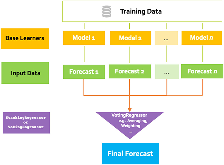
Figure 3. Fusion process according to the ensemble learning principle.

4. Results

Next, find a characterization of the observed forecast quality for key quantities of the weather forecast and the power output of the PV plant under investigation in terms of the graphical analysis and metrics outlined earlier, accompanied by a textual summary of the findings.

4.1. Forecast Quality of the Weather Prediction

The availability of both historical weather forecasts as well as measured climate data enables the evaluation of the weather forecasts' performance. Below, said performance in the time between summer solstice and winter solstice 2018 is evaluated at DWD station 10704 (near Saarlouis/Germany, located at an approximate distance of 8 km to the PV plants under investigation) for some of the quantities that are typically used as an input for PV performance forecasts, namely diffuse horizontal irradiance, air temperature, and wind speed. Additionally, the forecast quality for the global horizontal irradiance is evaluated because it is used for calculating the instantaneous clear sky index as outlined in section 2.2. Unfortunately, no measurements of direct horizontal irradiance are available and the forecast quality could therefore not be evaluated.

Scatter plots and histograms for global and diffuse horizontal irradiance shown in Figures 4A,B, respectively, reveal a wide spread of residuals and a tendency of the COSMO-D2-model to underestimate global and direct irradiance. The distribution of residuals for global horizontal irradiance is skewed toward negative values; in other words, forecast values are typically lower than measured values, especially for higher absolute values. The residual ranges from 543 to 413 W/m², with a mean of −62 W/m² and a standard deviation of 97 W/m².

FIGURE 4

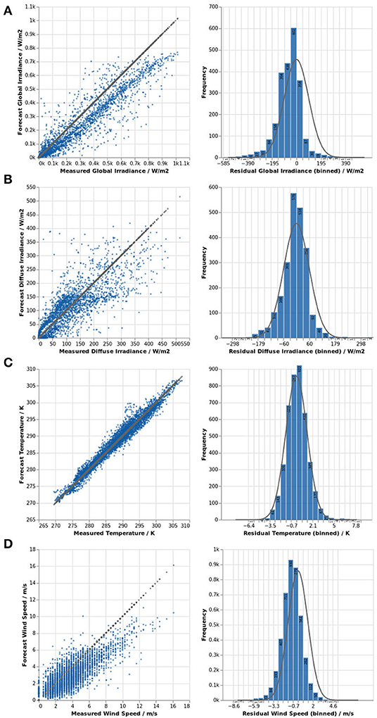
Figure 4. Forecast quality of the COSMO-D2 weather forecast at DWD station 10704 from 2018-06-21 – 2018-12-21: global horizontal irradiance (A), diffuse horizontal irradiance (B), air temperature, (C) and wind speed (D).

Forecasts for air temperature (Figure 4C) and wind speed (Figure 4D) are much better: temperature forecasts show a standard deviation of only 1.42 K and a maximum residual of 8 K. Forecasts for wind speed closely follow the expected normal distribution, which has a standard deviation of 1.32 m/s. The scatter plot indicates that higher wind speeds are much less common than wind speeds below 10 m/s. Also, forecasts seem to mostly underestimate higher wind speeds.

4.2. Overall Forecast Quality

Despite the general validity of the model, the uncertainty of the weather forecasts already suggests that the comparison between power forecast and measurements will show residuals that spread widely and can occasionally become large.

In Figures 5, 6, scatter plots of forecast and measurement over measured power and the histogram of residuals including a normal distribution with the same standard deviation as reference are shown for all forecast methods. Figure 7 shows forecasts for three perfectly sunny days in June to illustrate model deviations in absence of clouds.

FIGURE 5

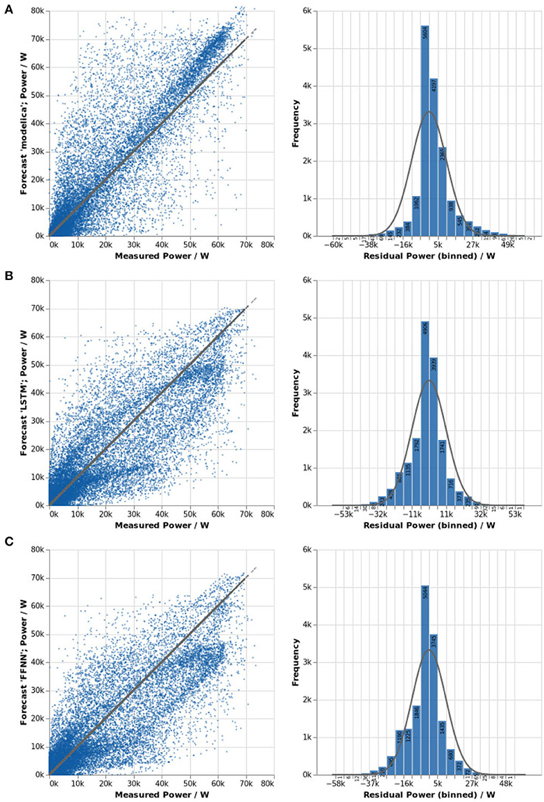
Figure 5. Forecast quality of the power forecast for site swsls-sw for 2019: physics-based (A), LSTM (B), and FFNN (C).

FIGURE 6

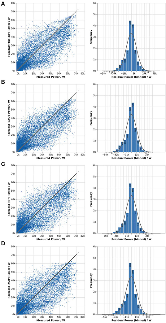
Figure 6. Forecast quality of the power forecast for site swsls-sw for 2019: fusion (A), BAG (B), RF (C), and XGB (D).

FIGURE 7

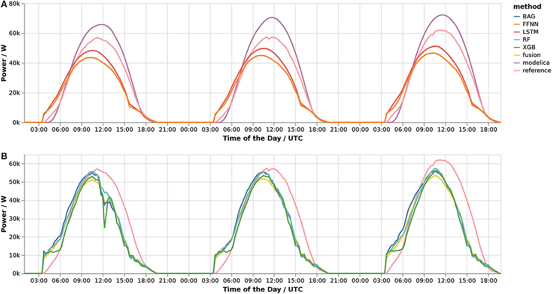
Figure 7. Forecasts and measurements for 2019-06-26 to 2019-06-28: physics-based, LSTM, and FFNN (A) as well as BAG, RF, XGB, and fusion (B).

For the physics-based PV array performance model, the scatter plot shows two clearly distinguishable clusters: one in the lower left-hand corner and one above the reference line in the top right. The first merely is a result of the fact that even after excluding all data points below 10 W, about 43% of the measured values fall in the bin from 10 to 9,275 W, which is the same for all forecast methods. The second cluster indicates that the model tends to overestimate the power produced above approximately 45 kW, which is reflected in a histogram that is clearly skewed to the right. One possible cause for this is panel aging, as the PV system under investigation has already been operational for 9 years in 2019.

For forecasts based on LSTM and FFNN, residuals follow the expected normal distribution more closely, but they are lightly skewed to the left. With the help of run plots on sunny days, the pattern resembling a hysteresis in the scatter plot can be interpreted: forecasts overestimate the power in the morning, and mostly underestimate the power around noon and in the afternoon. For higher wattages, the power is underestimated more often than it is overestimated (more accentuated for FFNN).

The identifier fusion denotes the forecast created by averaging all data-driven forecast methods. The averaging results in less widely spread residuals and a more symmetrical distribution of the residual closely following the normal distribution. When looking at run plots for sunny days, it becomes apparent that the averaging logically also extends to the strengths and weaknesses, which become less accentuated, which is good when strengths of some models increase average performance, but bad when weaknesses worsen average performance.

The scatter plot reveals that bagging had a tendency to overestimate the power output for low wattages, but rarely exceeded the measurements for high wattages above 55 kW. The distribution is slightly skewed to the right. Run plots for sunny days reveal that the model typically overestimates the power in the morning, but underestimates it in the afternoon; therefore, there is no accentuated skewedness of the histogram as both positive and negative residuals occur with similar rates.

The forecasts based on RF and XGB both underestimated high wattages above 50 kW much more often than they overestimated them, with XGB even showing a cluster at around 60 kW, indicating a limit of some sort. The run plots also show a significant overestimation in the morning and a consistent underestimation in the afternoon for sunny days.

Table 4 summarizes the findings of the residual analysis in terms of the metrics s and mm. In addition to the results for the forecasts of the power generated by the PV system, the weather forecasts and the results of the model validation are also included to provide additional context for interpretation of the values of s and mm. However, remember the differences between the different sites: for eugene-hit05667, the physics-based model was fed with about 3 months of measured environmental conditions to verify the validity of the model; for weather station 10704, weather forecasts of the numerical weather prediction model (NWP) COSMO-D2 were compared for half a year; and the forecast quality of the overall power forecast based on weather forecasts that were created at 21 UTC on the day before is evaluated for the year 2019 for swsls-sw.

TABLE 4

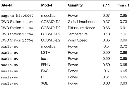
Table 4. Forecast performance for 2019 in terms of s and mm.

Figure 8 combines the information presented in Figures 5, 6 and Table 4 to render a graphical comparison of the different forecast methods. Each boxplot shows the distribution of the residuals: The boxes show the interquartile range (IQR) extending from Q₃ to Q₁, with the median value shown as white line inside the box. The whiskers indicate all values within 1.5*IQR above or below Q₁ and Q₃, respectively. The circles show values outside this range, which are considered outliers. For ranking, the metric mm was selected due to its emphasis on the similarity of the values' magnitudes.

FIGURE 8

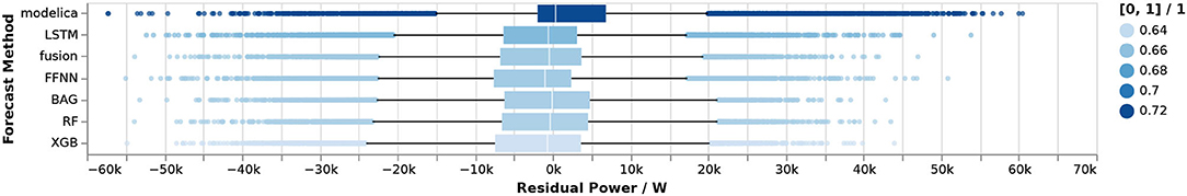
Figure 8. Boxplots of residual distribution for all methods; ranked and sorted by metric mm.

5. Discussion

In the previous section, the overall forecast performance for the AC power generated by a PV power plant was analyzed over the course of a year by means of residual analysis and selected metrics. Next, the results' implications are discussed.

5.1. Post-processing

First, the gained information on the accuracy (or lack thereof) of the forecasts in the past was used to quantify the uncertainty of newly created forecasts based on the assumption that the distribution of residuals remains about the same.

In Figure 9, a boxplot of the relative error for the physics-based PV array performance model in percent is shown for both the entire data set and each group of irradiance variability as estimated by the instantaneous clear sky index 1 − k_c. In this figure, the whiskers extend from the octile O₁ to O₇; all relative errors that fall in the first and last octile are omitted from the graph.

FIGURE 9

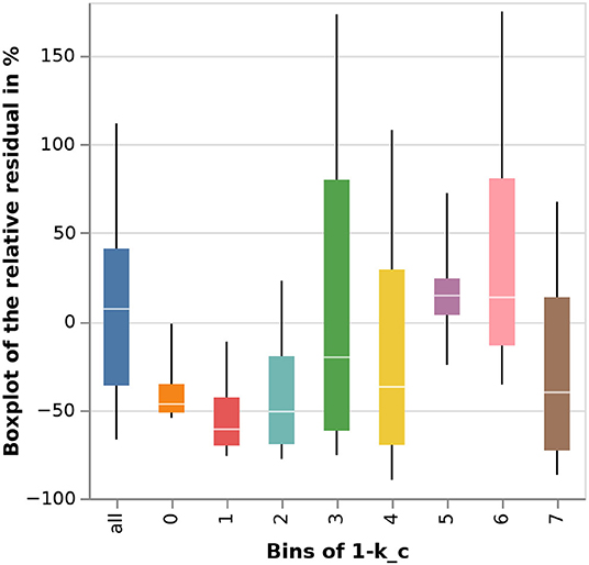
Figure 9. Forecast performance of the physics-based model in terms of the relative residual; overall and per bin of 1 − k_c.

Based on this information, Figure 10A shows the forecast for June 7, 2019, amended by a confidence band indicating the 50% (darker blue) and 75% (light blue) confidence level. Here, the confidence band is constructed from the overall relative residual. The forecast is visualized as a dashed line in dark blue; measurements are indicated by a line plot in dark gray. The plot indicates that while there is a specific forecast, the actual generated power will fall into the darker area with a likelihood of 50% and in the lighter area with a likelihood of 75%. Of course, measurements will still fall outside the confidence band, as can be seen in the beginning, in the early afternoon and in the evening on this exemplary day.

FIGURE 10

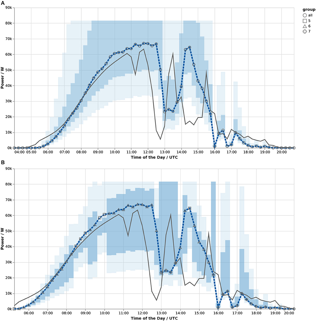
Figure 10. Physics-based forecast, error bands and measured power for June 7, 2019; extent of the confidence band based on overall performance (A) and bins of 1 − k_c (B).

Second, as shown in Figure 10B, the observed variability in the relative error clustered by 8 bins of the clear sky index 1 − k_c was used to construct the confidence band instead, as proposed by Meilinger et al. (2020). The symbols overlaid on the forecast encode the group in which the forecast clear sky index falls in at this time instant.

As a result, the confidence band narrows for groups in which better forecast performance was observed and widens for those with worse performance; moreover, it moves down if the forecasts predominantly overestimated the quantity and vice versa—as an example, consider the time before 10 a.m. in Figure 10. Theoretically, this should increase the accuracy of the information contained in forecast and confidence band. But, since the forecast of 1 − k_c logically exhibits its own uncertainties, it is unsure in how far this apparent improvement translates to the real world (compare Böök and Lindfors, 2020, section 4.2).

In addition to specifying the uncertainty of a forecast, information about the past performance could also be used to improve the forecast itself, for example by multiplying the forecast by $\frac{1}{1+Q_2}$ to correct a bias if there is one.

Böök and Lindfors (2020) instead suggest to adjust the forecast by “daily sets of independent adjustment coefficients C_N for each hour N,” which are calculated from the 90th percentiles of observed and forecasted power output in a sliding window of 30 days before the current date. This approach can, to some extent, compensate systematic errors not accounted for in the model, such as shadowing, inaccurate site metadata or systematic deviations in the environmental conditions at the site from the corresponding NWP. However, it might also be a viable way to further improve the forecast methods used in this work, as all of the data-driven models showed a consistent tendency to underestimate the output in the afternoon and the physics-based model instance constantly overestimated high wattages. Therefore, the presented approach presents an interesting opportunity for further work, but has not been explored yet.

5.2. Concluding Observations

In section 3, the underlying principles of the presented modeling approaches as well as their prerequisites were outlined: the physics-based model selected for this study is parameterized by five mandatory parameters, namely location, azimuth and tilt angle, total area and efficiency under reference conditions, and additional parameters for which default values can be used. In addition to the parameters (obtainable from data sheets or straightforward one-time measurements at the site), a model implementation and the means to simulate it are required; free and open-source implementations exist.

On the other hand, all data-driven forecasting approaches require measurements of the power output as well as historical weather forecasts used as input to the model. Provided these are available, the developed models are adaptable to other PV plants, according to the process shown in Figure 2. The models are applicable to small PV panels but also to large-size PV plants. In the context of smart grids, many small PV panels could be gathered virtually (for example in city quarters) to provide flexibility options. Gathering a large amount of small PV panels helps overcome the single forecasting limitations and provides a more robust generalized model.

For the scenario investigated in this work, all approaches showed similar performance in the same order of magnitude. Based on the selected metrics s and mm, the physics-based model performed best. However, it also resulted in the largest residuals and high wattages were consistently overestimated. The data-driven approaches based on neural networks, LSTM and FFNN, showed the second-best performance with less residuals considered outliers, but a clearly distinguishable tendency to underestimate the power output in the afternoon. The methods based on ensemble machine learning almost always underestimated wattages above 60 kW and less frequently resulted in small residuals. Additionally, the power output was consistently overestimated early in the morning.

With the availability of the system parameters shown in Table 3 and the lack of shadowing, the analysis performed suggests that the physics-based modeling approach is the first choice for a user that needs forecasts for small-scale PV systems that are connected to the low voltage grid or part of a microgrid. However, if these parameters do not exist and there is access to measurements of the power output and historical weather forecasts for training, FFNN and LSTM are viable approaches, too.

This result contrasts the findings of Ogliari et al. (2017), who concluded that physics-based models should be used for newly installed systems, followed by a hybrid modeling approach based on neural networks as soon as sufficient data becomes available, but both studies only considered one system, which relativizes the conclusions drawn.

From the perspective of local utility companies, it is more likely to readily have access to the measurements of power fed into their grid than it is to know the parameters necessary for the physics-based approach. Additionally, data-driven approaches suggest themselves in case there are shadows on the PV modules that are caused by immobile objects such as adjacent buildings. As long as the shadowing occurred in the training data, the methods will account for it. Adding a shadowing model to the physics-based model used in this work is possible, but severely complicates the finding of appropriate parameter values.

Because shadows are a reality on many systems, and because all approaches showed some degree of systematic errors, post-processing the created forecasts suggests itself. In this paper, the application of knowledge about the past forecast quality to specify the uncertainty of a forecast was discussed. Additionally, the suggestion by Böök and Lindfors (2020) represents another sensible post-processing step that could mitigate both shortcomings of the forecast method used as well as effects not accounted for in the model, such as shadowing, panel aging, soiling, or imprecise parameters.

6. Conclusion

In this work, a qualitative and quantitative analysis of the forecast performance for the entire year 2019 of different physics-based and data-driven forecast models for the power output of a 82 kWp PV system that is not subject to shadowing is presented. The data-driven models are trained on 5 years worth of data; the physics-based model is parameterized using non-optimized values measured on-site or obtained from data sheets.

The results show similar performance for all methods with a slightly better performance of the physics-based approach, suggesting that this method represents the first choice if the needed parameter values can be obtained. Since this requirement can likely not always be met in reality, data-driven approaches are also necessary, which in turn require measurements of the power generated and the historical weather forecasts for the training period. Both approaches create their forecast based on the output of numerical weather prediction models.

The work presented here shows the forecast quality to expect in similar situations and outlines how information about past forecast quality can be used to amend newly created forecasts by information about their inherent uncertainty. Possible areas for improvement include the optimization of the forecast methods themselves, the use of a more robust estimator for identifying classes of similar forecast performance, and the application of additional post-processing steps to further increase the accuracy of the forecasts.

Data Availability Statement

The data analyzed in this study is subject to the following licenses/restrictions: The measured power of the PV system analyzed in this article are provided by the local utility company Stadtwerke Saarlouis GmbH (SWSLS) for research purposes. The data set is not publicly available. Requests to access these datasets should be directed to moritz.stueber@aut.uni-saarland.de.

Author Contributions

MSt implemented the physics-based PV performance model in Modelica, designed and implemented the data analysis based on Python and pandas, and wrote the paper including all figures except section 3.2 and Figures 2, 3. FS contributed substantial work on implementation and testing of the software used to collect, process, and analyze data from varied sources. MD, AN, MSa, BB, and JB designed and implemented the data-driven forecast models, wrote the section 3.2, and reviewed the rest of the paper. GF discussed intermediate results throughout the investigation and reviewed the manuscript in detail. All authors contributed to the article and approved the submitted version.

Funding

This work was supported by the SINTEG-project “Designetz” funded by the German Federal Ministry of Economic Affairs and Energy (BMWi) under grant 03SIN224 and grant 03SIN222.

Conflict of Interest

The authors declare that the research was conducted in the absence of any commercial or financial relationships that could be construed as a potential conflict of interest.

Acknowledgments

The authors would like to thank the local utility company Stadtwerke Saarlouis GmbH (SWSLS) for supplying measurement data of the power output of two of the PV plants they operate, which made this work possible in the first place. Furthermore, we would like to thank Danny Jonas for an in-depth review of an earlier version of this paper.

Footnotes

1. ^https://www.dwd.de/EN/ourservices/opendata/opendata.html

2. ^https://www.dwd.de/EN/ourservices/nwp_forecast_data/nwp_forecast_data.html

3. ^https://meteotest.ch

4. ^https://doi.org/10.5281/zenodo.4392848

5. ^Compare Jonas et al. (2019, Table 2).

References

Ahmad, M. W., Mourshed, M., and Rezgui, Y. (2018). Tree-based ensemble methods for predicting PV power generation and their comparison with support vector regression. Energy 164, 465–474. doi: 10.1016/j.energy.2018.08.207

CrossRef Full Text | Google Scholar

Ahmed Mohammed, A., and Aung, Z. (2016). Ensemble learning approach for probabilistic forecasting of solar power generation. Energies 9, 2–17. doi: 10.3390/en9121017

CrossRef Full Text | Google Scholar

Böök, H., and Lindfors, A. V. (2020). Site-specific adjustment of a NWP-based photovoltaic production forecast. Solar Energy 211, 779–788. doi: 10.1016/j.solener.2020.10.024

CrossRef Full Text | Google Scholar

Choi, S., and Hur, J. (2020). An ensemble learner-based bagging model using past output data for photovoltaic forecasting. Energies 13, 2–16. doi: 10.3390/en13061438

CrossRef Full Text | Google Scholar

De Soto, W., Klein, S., and Beckman, W. (2006). Improvement and validation of a model for photovoltaic array performance. Solar Energy 80, 78–88. doi: 10.1016/j.solener.2005.06.010

CrossRef Full Text | Google Scholar

Dobreva, P., van Dyk, E. E., and Vorster, F. J. (2020). New approach to evaluating predictive models of photovoltaic systems. Solar Energy 204, 134–143. doi: 10.1016/j.solener.2020.04.028

CrossRef Full Text | Google Scholar

Faiman, D. (2008). Assessing the outdoor operating temperature of photovoltaic modules. Prog. Photovolt. Res. Appl. 16, 307–315. doi: 10.1002/pip.813

CrossRef Full Text | Google Scholar

Gao, M., Li, J., Hong, F., and Long, D. (2019). Day-ahead power forecasting in a large-scale photovoltaic plant based on weather classification using lstm. Energy 187:115838. doi: 10.1016/j.energy.2019.07.168

CrossRef Full Text | Google Scholar

Gashler, M., Giraud-Carrier, C., and Martinez, T. (2008). “Decision tree ensemble: Small heterogeneous is better than large homogeneous,” in 2008 Seventh International Conference on Machine Learning and Applications (San Diego, CA), 900–905. doi: 10.1109/ICMLA.2008.154

CrossRef Full Text | Google Scholar

Heydenreich, W., Muller, B., and Reise, C. (2008). “Describing the world with three parameters: a new approach to PV module power modelling,” in 23rd European Photovoltaic Solar Energy Conference and Exhibition (Valencia), 2786–2789.

Google Scholar

Holmgren, W. F., Hansen, C. W., and Mikofski, M. A. (2018). PVLIB python: a python package for modeling solar energy systems. J. Open Source Softw. 3:884. doi: 10.21105/joss.00884

CrossRef Full Text | Google Scholar

Hossain, M. S., and Mahmood, H. (2020). Short-term photovoltaic power forecasting using an lstm neural network and synthetic weather forecast. IEEE Access 8, 172524–172533. doi: 10.1109/ACCESS.2020.3024901

CrossRef Full Text | Google Scholar

Ineichen, P., and Perez, R. (2002). A new airmass independent formulation for the linke turbidity coefficient. Solar Energy 73, 151–157. doi: 10.1016/S0038-092X(02)00045-2

CrossRef Full Text | Google Scholar

Jonas, D., Lammle, M., Theis, D., Schneider, S., and Frey, G. (2019). Performance modeling of pvt collectors: implementation, validation and parameter identification approach using TRNSYS. Solar Energy 193, 51–64. doi: 10.1016/j.solener.2019.09.047

CrossRef Full Text | Google Scholar

Jonas, D., Theis, D., and Frey, G. (2018). “Implementation and experimental validation of a photovoltaic-thermal (PVT) collector model in TRNSYS,” in Proceedings of the 12th International Conference on Solar Energy for Buildings and Industry (EuroSun2018) (Rapperswil: International Solar Energy Society). doi: 10.18086/eurosun2018.02.16

CrossRef Full Text | Google Scholar

Kraiczy, M., Mey, B., Becker, H., von Berg, S. W., Braun, M., Hofbauer, P., et al. (2019). “PV forecasting in distribution system operation - requirements and applications,” in 9th Solar and Storage Integration Workshop (Dublin).

Marion, B., Anderberg, A., Deline, C., del Cueto, J., Muller, M., Perrin, G., et al. (2014). “New data set for validating pv module performance models,” in 2014 IEEE 40th Photovoltaic Specialist Conference (PVSC) (Denver, CO), 1362–1366. doi: 10.1109/PVSC.2014.6925171

CrossRef Full Text | Google Scholar

Massucco, S., Mosaico, G., Saviozzi, M., and Silvestro, F. (2019). A hybrid technique for day-ahead PV generation forecasting using clear-sky models or ensemble of artificial neural networks according to a decision tree approach. Energies 12:1298. doi: 10.3390/en12071298

CrossRef Full Text | Google Scholar

Meilinger, S., Yousif, R., Schroedter-Homscheidt, M., Herman-Czezuch, A., and Schirrmeister, C. (2020). “Wolkentypbedingte abweichung zwischen der gemessenen strahlungsvariabilitat und satellitengestatzten vorhersagemodellen,” in Tagungsunterlagen Online-PV-Symposium 2020.

Ogliari, E., Dolara, A., Manzolini, G., and Leva, S. (2017). Physical and hybrid methods comparison for the day ahead pv output power forecast. Renew. Energy 113, 11–21. doi: 10.1016/j.renene.2017.05.063

CrossRef Full Text | Google Scholar

Perez, R., Seals, R., Ineichen, P., Stewart, R., and Menicucci, D. (1987). A new simplified version of the perez diffuse irradiance model for tilted surfaces. Solar Energy 39, 221–231. doi: 10.1016/S0038-092X(87)80031-2

CrossRef Full Text | Google Scholar

Performance Modeling Collaborative (ed.). (2020). Modeling Steps. Available online at: https://pvpmc.sandia.gov/modeling-steps/

Ramsami, P., and Oree, V. (2015). A hybrid method for forecasting the energy output of photovoltaic systems. Energy Convers. Manage. 95, 406–413. doi: 10.1016/j.enconman.2015.02.052

CrossRef Full Text | Google Scholar

Reda, I., and Andreas, A. (2008). Solar position algorithm for solar radiation applications. Technical Report Number NREL/TP-560–34302. doi: 10.2172/15003974

CrossRef Full Text | Google Scholar

Richter, M., De Brabandere, K., Woyte, A., Kalisch, J., Schmidt, T., and Lorenz, E. (2015). “Uncertainties in pv modelling and monitoring,” in 31st European Photovoltaic Solar Energy Conference and Exhibition (Hamburg), 1683–1691.

Schroedter-Homscheidt, M., Kosmale, M., Jung, S., and Kleissl, J. (2018). Classifying ground-measured 1 minute temporal variability within hourly intervals for direct normal irradiances. Meteorol. Z. 27, 161–179. doi: 10.1127/metz/2018/0875

CrossRef Full Text | Google Scholar

Stein, J. S., Cameron, C. P., Borne, B., Kimber, A., Posbic, J., and Jester, T. (2010). A standardized approach to pv system performance model validation. doi: 10.1109/PVSC.2010.5614696. Available online at: https://www.osti.gov/biblio/1141557

CrossRef Full Text | Google Scholar

Toet, A., Tak, S., and Erp, J. (2016). Visualizing uncertainty. towards a better understanding of weather forecasts. Tijdschrift voor Human Factors 41, 9–14. Available online at: http://resolver.tudelft.nl/uuid:9a069a89-0cf3-4c3b-801d-aab4501d32ce

Google Scholar