 Peixiao Sun
 Zaibin Jiao*
- Department of Electrical Engineering, Xi’an Jiaotong University, Xi’an, China
The calculation of the short-circuit current is an important basis for fault detection and equipment selection in the DC distribution system. This paper proposes a linearized model for modular multilevel converter (MMC) considering different grounding methods and different failure scenarios. This model can be used in different fault conditions before MMC’s block. Under different fault forms, the model has different manifestations. This paper analyzes and models the DC distribution network with two types of faults: inter-pole short circuit and single-pole grounding short circuit. Among them, the modeling and analysis of single-pole grounding short-circuit uses the method of common- and differential-mode (CDM) transformation. To solve such a model, an analytical calculation method is proposed. As a mean of evaluating the effectiveness and accuracy of the proposed model, the analytical calculation solution is compared to the solution produced by PSCAD/EMTDC. A comparison of the results reveals the efficacy of the proposed model.
Introduction
With the continuous development of society, people's production methods are becoming more and more abundant, and the demand for the use of electric energy is also increasing. At present, the AC distribution network in some large cities is facing the problem of lack of power supply corridors and insufficient power supply capacity. At the same time, the traditional AC distribution network has problems such as three-phase imbalance and insufficient node reactive power support, which are becoming more and more prominent under the trend of substantial increase in electricity demand. In addition, the rise of many high-tech industries has put forward higher requirements for power supply reliability and power quality. However, high-quality power supply is difficult to achieve due to problems such as harmonics and shock loads caused by converter equipment in the network. This series of problems has promoted the technological innovation of the distribution network (Feng, 2019).
As countries attach importance to renewable energy and the development of power electronics technology, DC power distribution technology has gradually entered people's field of vision. At the same time, the DC distribution network has become a feasible way to solve a series of problems in the traditional AC distribution network with its advantages of large transmission capacity, low line cost, low network loss, high power supply reliability and high power quality (Baran and Mahajan, 2003; Sannino et al., 2003; Starke et al., 2008). What’s more, the DC distribution network with converters and a series of power electronic equipment is highly controllable and would be an important part of flexible and active distribution networks. In the DC distribution network, the converter is one of the key equipment. As a new generation of converters, voltage source converter has the advantages of the ability to manage power flow direction, immunity against commutation failure and easy extension to multi-terminal DC grid (Lyu et al., 2016; Hao et al., 2019). Therefore, the voltage source converter provides the possibility for the DC distribution network. At present, as a kind of voltage source converters, MMC not only has high output waveform quality, but also has low switching frequency and low loss (Xu, 2013). It is currently the key research object of DC technology.
The calculation of the short-circuit current is an important basis for fault detection and equipment selection in the DC distribution system (Li et al., 2018). At present, many researchers have studied the calculation of DC short-circuit current in the DC distribution network formed by MMCs. Franquelo et al. (2008) conducted a qualitative analysis of various types of faults in the multi-terminal DC grid composed of MMCs. Some researchers applied simulation methods to analyze the short circuit on the DC side of the MMC (Bucher and Franck, 2013; Zhang and Xu, 2016; Han et al., 2018; Tünnerhoff et al., 2018). Although such simulation is accurate, the modeling is complicated and time-consuming, so it is not suitable for system planning and design. In order to avoid these shortcomings of simulation, we can use a simplified model for analytical calculations. Zhou et al. (2017) conducted a theoretical analysis of the DC distribution network formed by MMC when the DC side was not grounded, and investigated the equivalent discharge circuit before the MMC is blocked after a short-circuit fault occurred at the outlet of the MMC and a single-pole grounding fault. Based on the circuit model of the equivalent discharge loop, the analytical expression of the fault discharge current is derived. Xu (2013) analyzed the equivalent circuit of the MMC before the MMC is blocked when the output of the MMC is short-circuited. In his research, the steady-state situation after MMC’s block was solved and the analytical expression of the whole fault process is revealed. In addition, Xu (2013) also introduced a circuit model that applies the superposition theorem to calculate when facing a complex topology of a multi-terminal DC grid, and simulated the calculation model. In (Wang et al., 2011), the discharge circuit of the sub-module after the inter-electrode short circuit at the outlet of the MMC was divided into two stages before and after the MMC is locked, and the analytical expression of the sub-module overcurrent was presented. Gao et al. (2020) applied a converter model composed of an RLC series circuit and a parallel current source, and performed an effective approximate calculation of the short circuit between poles. Shi and Ma (2020) analyzed the fault circuit under a single-pole grounding short circuit, and calculated the short-circuit current for a two-terminal DC system.
From the previous discussion, in the DC distribution network that widely adopts symmetrical unipolar structure wiring, people have more abundant researches on short-circuit faults between poles at the outlet of MMC, but less on single-pole grounding faults. In addition, when a failure occurs at the line, it is difficult to derive the analytical expression of the fault current in the face of a complex multi-terminal DC system, and the calculation method lacks more detailed research.
To bridge these gaps, this paper presents the linearized model before MMC’s block in two types of faults. In addition, for the complex multi-terminal DC distribution network model, an effective solution method is proposed.
The rest of this paper is organized as follows. In Analysis and Modeling of DC Distribution System, a model of DC distribution system is presented. In Model Solution Method, a method to solve the presented model is proposed. In Case Studies, case studies are conducted to evaluate the effectiveness and accuracy of the proposed model. Concluding remarks are presented in Conclusion.
Analysis and Modeling of DC Distribution System
The topology of MMC is shown in Figure 1. Because the fault characteristics of various sub-modules are basically the same before the MMC is locked, the half-bridge sub-module is taken as a representative here. MMC is a converter that relies on constant switching between sub-modules to approximate a sine wave with a step wave, so MMC is a time-varying circuit. However, if we make the analysis time short enough and believe that the MMC input and bypass sub-modules remain unchanged, we can regard MMC as a linear and time-invariant circuit and use the superposition theorem for analysis. The following research work is based on this assumption.
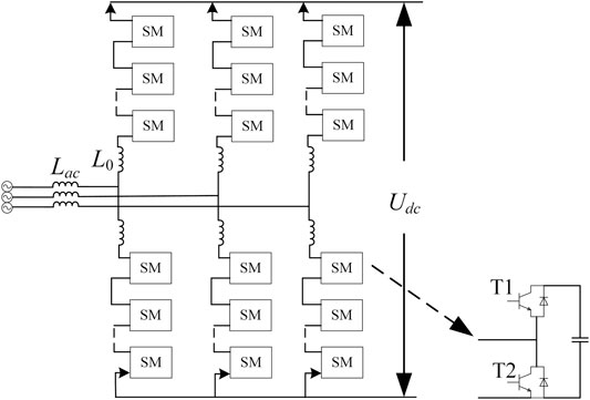
FIGURE 1. The topology of MMC.
Analysis and Modeling Under Inter-pole Short-Circuit Faults
When an inter-pole short-circuit fault occurs in a DC distribution network, the superposition theorem can be used at the fault point f to divide the inter-pole voltage at the fault point into a normal component and a fault component, as shown in Figure 2. Then the response generated by all other excitation sources except the fault component voltage at the fault point is the response of the normal operating state of the circuit. Under the normal operating state, the short-circuit current at the fault point is zero, and the current carried by each line is the current under normal operation. The current under normal operating conditions can be obtained by load flow calculation or direct measurement, and will not be calculated in this article. This paper will calculate the fault component current, which is the zero state response current of the circuit under the excitation of the fault component power supply. If there is no transition resistance, the fault component power supply can be regarded as a voltage source. If there is a transition resistance at the fault point, the fault component current can be expressed by the response under the excitation of the fault component current source. This current source can be obtained by transforming the fault component voltage source and transition resistance through Norton's equivalent law.
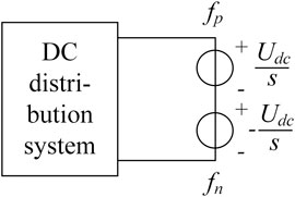
FIGURE 2. Schematic diagram of the superposition theorem.
When considering the zero-state response of the fault component voltage source in the circuit, MMC can be transformed into an equivalent circuit model as shown in Figure 3. R, L, and C in the model are all calculated by Eq. 1 (Xu, 2013). If the MMC is grounded through the midpoint of the capacitor, the corresponding capacitance value can be added to C.
Where R0 and L0 are the resistance and inductance of the bridge arm reactor, respectively, Rdc and Ldc are the resistance and inductance of the smoothing reactor at the converter outlet, respectively, N is the number of sub-modules in each bridge arm, and C0 is the sub-module capacitance.
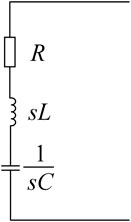
FIGURE 3. Zero-state response equivalent circuit model of MMC in frequency domain.
The DC line can be described as a π-type equivalent circuit model. In order to make the subsequent calculation easier, the parameters of the model are converted to the positive pole or inter-pole, as shown in Figure 4. When calculating with the positive pole current and the voltage between poles, the model before and after the conversion is equivalent.
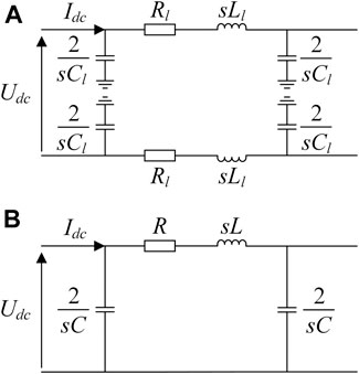
FIGURE 4. Equivalent circuit model before and after conversion of DC line (A) Before conversion. (B) After conversion.
In Figure 4, Rl, Ll and Cl are the equivalent resistance, equivalent inductance, and equivalent capacitance of the positive/negative line, respectively. R, L and C in Figure 4 are their values after converted to the positive pole or inter-pole. The circuit parameters before and after conversion have the following relationship:
Analysis and Modeling Under Single-Pole Grounding Faults
When a single-pole grounding fault occurs, the transient characteristics of the DC distribution network are greatly affected by the grounding method of the AC and DC sides. There will be different fault loops and fault mechanisms under different grounding methods on the AC and DC sides of the DC distribution network. Therefore, before modeling, it is necessary to classify the different grounding methods of the AC and DC sides of the MMC. If there is a zero-sequence path on the AC side of the MMC, the AC side is considered to be grounded. Otherwise, it is considered that the AC side is not grounded. As shown in Figure 5, MMC's DC side grounding methods are divided into three types: ungrounded, grounded through the midpoint of the clamp resistance, and grounded through the midpoint of the capacitor (Luo, 2019).
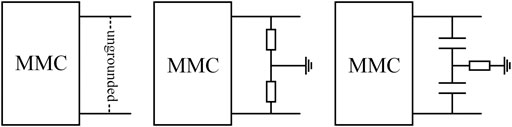
FIGURE 5. MMC's DC side grounding method.
When modeling the MMC, in order to make the model symmetric about the positive and negative poles, and to facilitate subsequent analysis and calculation, the influence of the bridge arm reactor was ignored. Considering that the inductance of the bridge arm reactor is not too large, it is generally an order of magnitude smaller than the inductance of the smoothing reactor at the converter outlet, so the error caused by the simplified model will not be large, and the conservativeness of the model can also be taken into account.
Under different grounding modes, the zero-state response equivalent circuit of MMC is shown in Figure 6. The dashed line indicates that the connection exists only when the AC and DC sides of the MMC are grounded in a corresponding way. Lac represents 1/3 of the zero-sequence inductance on the AC side when the AC side is grounded (Luo, 2019). Rg represents the clamp resistance. Cg represents grounding capacitance. Rcg represents the ground resistance at the midpoint of the capacitor.
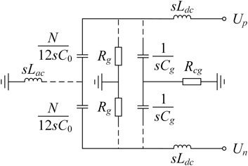
FIGURE 6. The zero-state response equivalent circuit model of MMC under single-pole grounding faults.
The DC line can be described as the unconverted equivalent circuit model in Figure 4.
The single-pole grounding short circuit will make the circuit asymmetrical. Therefore, we can analyse it with CDM conversion. From the perspective of CDM, it will be divided into two symmetrical circuits that are easy to analyze. The CDM conversion has the following mathematical form (Kimbark, 1970):
Where Σ and Δ respectively represent common-mode and differential-mode components. In addition, p and n respectively represent positive and negative parameters. This formula is applicable to both current and voltage.
After CDM conversion of current and voltage, the converter model will become the following form:
(1) Case 1: The AC side is not grounded, and the DC side is grounded through the midpoint of the capacitor.
In this case, the common-mode and differential-mode models of the converter are shown in Figure 7.
(2) Case 2: The AC side is not grounded, and the DC side is grounded through the midpoint of the clamp resistor.
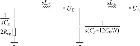
FIGURE 7. The common-mode (left) and differential-mode (right) models of the converter in case 1.
In this case, the common-mode and differential-mode models of the converter are shown in Figure 8. When the DC side is not grounded, it is equivalent to an open circuit at Rg, so it will not be listed separately later.
(3) Case 3: The AC side is grounded, and the DC side is grounded through the midpoint of the capacitor.
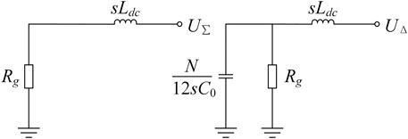
FIGURE 8. The common-mode (left) and differential-mode (right) models of the converter in case 2.
In this case, the common-mode and differential-mode models of the converter are shown in Figure 9.
(4) Case 4: The AC side is grounded, and the DC side is grounded through the midpoint of the clamp resistor.
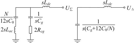
FIGURE 9. The common-mode (left) and differential-mode (right) models of the converter in case 3.
In this case, the common-mode and differential-mode models of the converter are shown in Figure 10. When the DC side is not grounded, it is equivalent to an open circuit at Rg, so it will not be listed separately later.
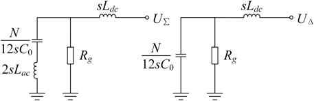
FIGURE 10. The common-mode (left) and differential-mode (right) models of the converter in case 4.
After CDM conversion of current and voltage, the DC line model is shown in Figure 11. Its common-mode model is the same as Its differential-mode model.
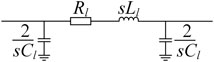
FIGURE 11. The CDM model of the DC line.
From the perspective of CDM, the fault boundary conditions of the circuit also need to be converted. Without loss of generality, if we set a negative pole grounding short-circuit fault at the fault point f, the boundary conditions can be expressed as Eq. 4.
Where Uf,n is the negative voltage at the fault point, If,p and If,n are the positive and negative currents flowing from the fault point to the ground, respectively, and Rf is the transition resistance between the fault point and the ground.
Through CDM transformation of Eq. 4, the boundary conditions are transformed into Eq. 5.
Where Uf,∑ and Uf,Δ are the common-mode and differential-mode voltage at the fault point, respectively, If,∑ and If,Δ are the common-mode and differential-mode current flowing from the fault point, respectively.
Similar to the asymmetric fault analysis of the AC grid, the DC distribution network also has the following relationships at the fault point:
Where
In Eq. 6, Uf,Δ(0) is the normal component of the differential-mode voltage at the fault point, ZΔ and Z∑ are the equivalent differential-mode and common-mode impedance of DC distribution network measured from the fault point, respectively. In Eq. 7, Udc is the inter-pole voltage at the fault point during normal operation.
According to Eq. 5 and Eq. 6, an equivalent CDM network as shown in Figure 12 can be formed.
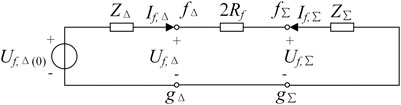
FIGURE 12. The equivalent CDM network under single-pole grounding fault.
Model Solution Method
Solution of Fault Component Current Under Inter-pole Short-Circuit Faults
Since it is difficult to derive analytical formulas for high-order circuits when the DC distribution network has a complex topology, this section introduces an analytical calculation method suitable for computers. The symbolic math toolbox of MATLAB can help us use this method.
Before the calculation, the circuit structure should be classified, and the buses should be classified first:
(1) Voltage bus: The fault component voltage of the bus is known, while the fault component injection current at the bus is unknown. This kind of bus is generally at the fault point.
(2) Current bus: The fault component injection current at the bus is known, while the fault component voltage of the bus is unknown. This kind of bus is generally a non-fault bus or at a fault point with a known fault component current.
After that, the connection structure in the circuit also needs to be classified:
(1) Grounding structure
The grounding structure is shown in Figure 13. The ground in the figure is not the ground in the conventional sense, but the reference point of the bus voltage. In this calculation for the inter-pole short-circuit fault, the inter-pole voltage and the positive current are used for calculation, so the ground in Figure 13 is equivalent to the converted negative circuit in Figure 4.
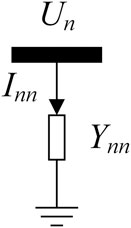
FIGURE 13. The grounding structure.
The inter-pole voltage Un and the positive current Inn in the grounding structure have the following relationship:
Where Ynn is the admittance of grounding structure.
(2) Bus connection structure
The bus connection structure is shown in Figure 14.
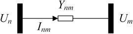
FIGURE 14. The bus connection structure.
Un and Um are the inter-pole voltage at the bus n and m, respectively. The positive current flowing in the bus connection structure Inn and they have the following relationship:
After classifying the structure of the DC distribution network, the fault component current can be solved under the inter-pole short-circuit fault. The following matrix has been defined and used as input of the calculation formula.
Assuming that there are Nb original buses in the circuit, the circuit will have Nb+1 buses after adding a faulty bus (if the fault occurs at an original bus, the number of buses will not change).
(1) Connection matrix F ((Nb+1)×(Nb+1)): It describes the connection of the DC distribution network:
i) Fnm = 1, if a line connects buses n and m.
ii) Fnm = 0, if no line connects buses n and m.
(2) Admittance matrix Y ((Nb+1)×(Nb+1)): The diagonal element Ynn in the matrix is the ground admittance at bus n, and the non-diagonal element Ynm is the admittance of the DC line connecting buses n and m.
With input matrices F and Y, according to KVL and KCL, we can list the following linear equations at ni current buses.
Where
In the equation set shown in Eq. 10, there are ni current bus voltages as variables, and this number is the same as the number of equations. Therefore, the expression of the unknown voltage in the frequency domain can be solved by a computer.
After obtained the voltage of each bus, Eq. 11 can be used to determine the fault component current flowing out of the MMC’s outlet at bus n.
Where Rc-n, Lc-n and Cc-n are the resistance, inductance and capacitance in the MMC equivalent circuit at bus n, respectively.
The fault component current flowing from bus n to bus m can be determined by Eq. 12.
Where Rl-nm, Ll-nm and Cl-nm are the resistance, inductance and capacitance in the DC line equivalent circuit between bus n and bus m, respectively.
Then, Eq. 13 can be used to determine the inter-pole short-circuit current flowing from the positive pole at the fault point f.
After calculated the fault component currents everywhere, we can use a computer to perform the inverse Laplace transform to obtain the corresponding time-domain expression.
Solution of Fault Component Current Under Single-Pole Grounding Short-Circuit Faults
To solve the fault component current in this case, the CDM currents at the fault point should be calculated first. According to the circuit shown in Figure 12, the common-mode current If, Σ and the differential-mode current If, Δ flowing from the fault point can be solved by Eqs. 14,15.
Where
In Eqs. 16,17, Y∑ and YΔ are the common- and differential-mode admittance matrixes, respectively.
After obtaining If, Σ and If, Δ, the solution methods mentioned in the calculation of inter-pole short-circuit can be applied to solve the common- and differential-mode networks respectively. Here, the CDM voltages and currents excited by the fault component current source should be used as unknown variables. After that, the positive and negative currents of the fault components can be obtained through the inverse CDM transformation shown in Eq. 18.
Finally, the time-domain expression of the fault component current can be obtained through the inverse Laplace transform.
Case Studies
This section presents the case studies that were used for evaluating the effectiveness and accuracy of the proposed linearized model. We will compare the calculated value and the simulated value in the four-terminal ring grid DC distribution system shown in Figure 15. This simulation value is provided by PSCAD/EMTDC. Table 1 provides the corresponding system parameters. The system adopts master-slave control strategy. MMC1 is the master station, and the rest are slave stations. The active powers in the table are the injected powers on the AC side. The injected reactive power of each MMC is zero.
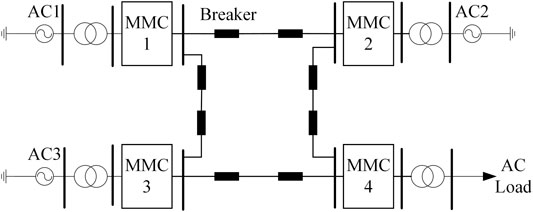
FIGURE 15. The four-terminal ring grid DC distribution system.
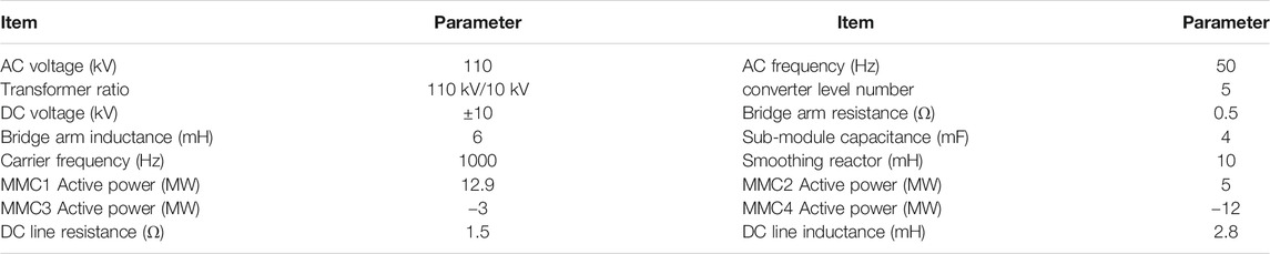
TABLE 1. The system parameters of four-terminal ring grid DC distribution system.
Verification Under Inter-pole Short-Circuit Faults
In the verification under inter-pole short-circuit faults, all the MMCs in Figure 15 are not grounded, and the transition resistance is zero. After the circuit is stable, set an inter-pole short circuit at the midpoint of the DC line between MMC1 and MMC2 (let t = 0s at this time). The short-circuit currents obtained are shown in Figure 16.
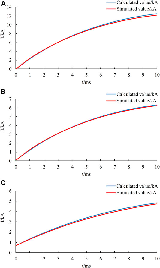
FIGURE 16. Comparison of the calculated value and the simulated value of the fault current during a inter-pole short circuit (A) Short circuit current at fault point. (B) Positive current flowing from MMC1 to MMC2 on the fault line. (C) Positive current at the outlet of MMC1.
From the comparison in Figure 16, it can be seen that compared to the simulated value, the calculated value has a small error (no more than 2.64%), and this error would gradually increase over time. I think the reason for this error is that the MMC will no longer maintain the original operating state after the fault, the steady-state component of the fault current would change, and this change would gradually increase over time. Therefore, the calculation method using the superposition theorem in the previous article is only applicable in a very short time after the failure. However, considering that the MMC will be blocked within a very short time after a DC failure, the calculation result is still quite reliable within this time.
Verification Under Single-Pole Grounding Short-Circuit Faults
In the verification under single-pole grounding short-circuit faults, to verify the MMC models of different grounding methods, the MMCs in Figure 15 are set with different grounding methods. For MMC1, the AC side is grounded (Lac = 10mH), and the DC side is grounded through the midpoint of the capacitor (Cg = 8mF, Rcg = 0.5Ω). For MMC2, the AC side is not grounded, and the DC side is grounded through the midpoint of the clamp resistor (Rg = 4MΩ). For MMC3, the AC side is not grounded, and the DC side is grounded through the midpoint of the capacitor (Cg = 8mF, Rcg = 0.5Ω). For MMC4, the AC side is grounded (Lac = 10mH), and the DC side is grounded through the midpoint of the clamp resistor (Rg = 4MΩ). After the circuit is stable, set a negative ground short circuit (Rf = 0) at the midpoint of the DC line between MMC1 and MMC2 (let t = 0s at this time). The short-circuit currents obtained are shown in Figure 17.
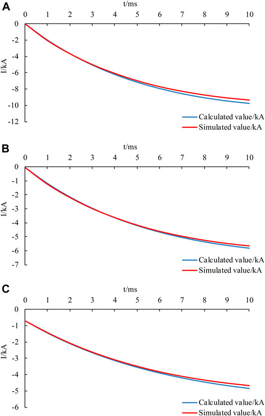
FIGURE 17. Comparison of the calculated value and the simulated value of the fault current during a negative ground short circuit (A) Short circuit current at fault point. (B) Negative current flowing from MMC1 to MMC2 on the fault line. (C) Negative current at the outlet of MMC1.
From the comparison in Figure 17, it can be seen that compared to the simulated value, the calculated value has a small error (no more than 4.53%), and this error would gradually increase over time. Not only that, the error in this calculation is larger than that in the calculation of inter-pole short-circuit fault. I think the error in this calculation is not only related to the change in the operating state of the MMC, but also related to the neglect of the bridge arm reactor. This calculation result is not only reliable in a very short time, but also conservative.
Conclusion
This paper summarizes the MMC model in the calculation of inter-pole short circuit, and proposes a new linearized model based on CDM transformation for single-pole grounding short-circuit calculation. Through verification with simulation results, this new model is proven to be reliable and conservative. In addition, this paper proposes a frequency domain calculation method suitable for the calculation of complex multi-terminal DC distribution networks. This method can flexibly transform the network topology and has a much faster calculation speed than simulation. The models and method in this paper can be used as a reference for grid planning and equipment selection.
Data Availability Statement
The raw data supporting the conclusions of this article will be made available by the authors, without undue reservation.
Author Contributions
PS: analysis, modeling, method, verification and writing. ZJ: advising, supervision, writing-reviewing and editing. HG: simulation model, conceptualization and methodology.
Conflict of Interest
The authors declare that the research was conducted in the absence of any commercial or financial relationships that could be construed as a potential conflict of interest.
References
Baran, M. E., and Mahajan, N. R. (2003). DC distribution for industrial systems opportunities and challenges. IEEE Transactions on Industry Applications 39 (6), 1596–1601. doi:10.1109/TIA.2003.818969
Bucher, M. K., and Franck, C. M. (2013). Contribution of fault current sources in multiterminal HVDC cable networks. IEEE Transactions on Power Delivery 28 (3), 1796–1803. doi:10.1109/TPWRD.2013.2260359
Feng, T. (2019). Research on transient analysis grounding mode and fault flexible medium voltage DC distribution network. Master’s Thesis, China: Xi'an University of Technology.
Franquelo, L. G., Rodriguez, J., Leon, J. I., Kouro, S., Portillo, R., and Prats, M. A. M. (2008). The age of multilevel converters arrives. IEEE Industrial Electronics Magazine 2 (2), 28–39. doi:10.1109/MIE.2008.923519
Gao, S., Ye, H., and Liu, Y. (2020). Accurate and efficient estimation of short-circuit current for MTDC grids considering MMC control. IEEE Transactions on Power Delivery 35 (3), 1541–1552. doi:10.1109/TPWRD.2019.2946603
Han, X., Sima, W., Yang, M., Li, L., Yuan, T., and Si, Y. (2018). Transient characteristics under ground and short-circuit faults in a ±500kV MMC-based HVDC system with hybrid DC circuit breakers. IEEE Transactions on Power Delivery 33 (3), 1378–1387. doi:10.1109/TPWRD.2018.2795800
Hao, Q., Li, Z., Gao, F., and Zhang, J. (2019). Reduced-order small-signal models of modular multilevel converter and MMC-based HVdc grid. IEEE Transactions on Industrial Electronics 66 (3), 2257–2268. doi:10.1109/TIE.2018.2869358
Kimbark, E. W. (1970). Transient overvoltages caused by monopolar ground fault on bipolar DC line: theory and simulation. Power Apparatus Systems IEEE Transactions on PAS 89 (4), 584–592. doi:10.1109/TPAS.1970.292605
Li, C., Gole, A. M., and Zhao, C. (2018). A fast DC fault detection method using DC reactor voltages in HVdc grids. IEEE Transactions on Power Delivery 33 (5), 2254–2264. doi:10.1109/TPWRD.2018.2825779
Luo, F. (2019). Research on grounding method and protection strategy of DC distribution network for power supply in remote areas. Master’s Degree, China: Xi’an Jiaotong University.
Lyu, J., Cai, X., and Molinas, M. (2016). Frequency domain stability analysis of MMC-based HVdc for wind farm integration. IEEE J. Emerging and Selected Topics in Power Electronics 4 (1), 141–151. doi:10.1109/JESTPE.2015.2498182
Sannino, A., Postiglione, G., and Bollen, M. H. J. (2003). Feasibility of a DC network for commercial facilities. IEEE Transactions on Industry Applications. 39 (5), 1499–1507. doi:10.1109/TIA.2003.816517
Shi, X., and Ma, J. (2020). “Analysis of DC-side single Pole grounding fault in MMC-HVDC system considering the influence of control strategy,” in 2020 12th IEEE PES Asia-Pacific Power and Energy Engineering Conference, Nanjind, China, September 20–23, 2020. doi:10.1109/APPEEC48164.2020.9220729
Starke, M. R., Tolbert, L. M., and Ozpineci, B. (2008). “AC vs. DC distribution: a loss comparison,” in Transmission and Distribution Conference and Exposition, 2008, Chicago, IL, April 21–24, 2008. doi:10.1109/TDC.2008.4517256
Tünnerhoff, P., Ruffing, P., and Schnettler, A. (2018). Comprehensive fault type discrimination concept for bipolar full-bridge-based MMC HVDC systems with dedicated metallic return. IEEE Transactions on Power Delivery 33 (1), 330–339. doi:10.1109/TPWRD.2017.2716113
Wang, S., Zhou, X., Tang, G., He, Z., Teng, L., and Bao, H. (2011). Analysis of submodule overcurrent caused by DC pole-to-pole fault in modular multilevel converter HVDC system. Proceedings of the CSEE 31 (01), 1–7. doi:10.13334/j.0258-8013.pcsee.2011.01.001
Zhang, Z., and Xu, Z. (2016). Short-circuit current calculation and performance requirement of HVDC breakers for MMC-MTDC systems. IEEJ Transactions on Electrical and Electronic Engineering 11 (2), 168–177. doi:10.1002/tee.22203
Keywords: DC distribution system, short-circuit current calculation, MMC, linearization, common- and differential-mode
Citation: Sun P, Jiao Z and Gu H (2021) Calculation of Short-Circuit Current in DC Distribution System Based on MMC Linearization. Front. Energy Res. 9:634232. doi: 10.3389/fenrg.2021.634232
Received: 27 November 2020; Accepted: 18 January 2021;
Published: 04 March 2021.
Edited by:
Peng Li, Tianjin University, ChinaCopyright © 2021 Sun, Jiao and Gu. This is an open-access article distributed under the terms of the Creative Commons Attribution License (CC BY). The use, distribution or reproduction in other forums is permitted, provided the original author(s) and the copyright owner(s) are credited and that the original publication in this journal is cited, in accordance with accepted academic practice. No use, distribution or reproduction is permitted which does not comply with these terms.
*Correspondence: Zaibin Jiao, amlhb3phaWJpbkB4anR1LmVkdS5jbg==