Control Rod Drop Hydrodynamic Analysis Based on Numerical Simulation

The drop time of the control rod plays an important role in judging whether a nuclear reactor can be safely shut down in an emergency condition and has become one of the most important parameters for the safety analysis of nuclear power plants. Exact assessment of the drop time is greatly dependent on the forces acting on the control rod. In this research, a three-dimensional numerical simulation of the control rod in a low-temperature heating reactor was established based on 6DOF (6 degrees of freedom) model using dynamic meshing technology, and it was used to analyze the control rod dropping experiment. The behavior of dropping the control rod was obtained, including the velocity, the displacement, and the pressure distribution on the control rod guide tube. The comparison between the simulation and the experiment results indicated that the simulation was capable of simulating the dropping characteristic of the control rod. Some important parameters can be calculated, such as the time of control rod dropping process and the maximum impact force. Based on this, useful information could be provided for the design of control rod driveline structure.

Introduction

The reactor control rod assembly is generally set up with a star frame and several control rods. Each control rod assembly has its own drive system, which can act individually or act in groups with other control rods, therefore ensuring the ability to control the startup and shutdown of the reactor, power change, and fast reactivity change to protect the reactor. The control rod drive mechanism is required to move slowly under normal working conditions to ensure the safety of the reactor; in the case of an accident, the driving mechanism can be automatically detached so that the control rod assembly can be quickly inserted into the core under the gravity. The whole process can be completed in 2–3 s. If the control rod drops too slowly or the control rod assembly corresponding to the component with the highest reactivity yield fails to act during the emergency shutdown, a set of serious accidents can be generated. Therefore, to ensure the safety of the reactor, the shutdown time must meet the specified time requirements (Chen and Liu, 2007). Under the first and second working conditions of the reactor, the drop time according to the safety standards of the control rods is less than 3.5 s (Yoon et al., 2009). In some nuclear power plant designs, the time of dropping to falling of the control rod into the inlet of the guide tube buffer section is within 2 s.

Therefore, in terms of reactor safety analysis, the drop time of control rod plays an important role in determining whether a nuclear reactor can be safely shut down in an emergency and has become one of the important parameters of nuclear power plant safety analysis. If the drop time of the control rod is considered only without other matters, it is generally expected to be as short as possible. However, the reduction of drop time will lead to a higher speed of control rod assembly. After falling into the fuel assembly, the control rod assembly rapidly falling will have a great impact on the fuel assembly and even the in-pile structure, thence causing damage to the control rod assembly itself and other related components. The control rod guide tube provides a passage for inserting and withdrawing the control rod. In the lower part of the guide tube, the diameter of the positioning frame between the first and second layer is reduced to make sure it can display a buffer role when the control rod is about to approach the bottom of the guide tube, thence striving to prevent the impact of the falling rod from damaging other components in the stack while ensuring that the rod drop time meets the safety requirements. The force performance of dropping the control rod is complicated. The rod drop time is directly related to its structural design, manufacture, and installation and is also affected by the coolant state, core temperature, core pressure, and external load during falling. To solve the problem of rod drop time, scholars from different countries have studied mechanical friction resistance, fluid resistance, external excitation, fluid-solid coupling, and other complex problems (Su et al., 1977; Stabl and Ren, 1999; Qu and Chen, 2001; Yu et al., 2001; Sun et al., 2003; Peng et al., 2013) in rod dropping process. However, due to the complexity of these physical mechanisms, relevant researches often combine theoretical derivation with empirical formula, and there are many simplifications and assumptions, and a large number of correction coefficients related to experiments are introduced, so the expansion of special software is poor (Collard, 1999). The control rod assembly and the working environment of pool atmospheric low-temperature heating reactor are different from commercial pressurized water reactors. The special software or empirical relation applicable to the rod drop analysis of commercial pressurized water reactor will not be applicable to the pool-type atmospheric pressure low-temperature heating reactor. However, the dynamic mesh technology of the fluid dynamics simulation software FLUENT can effectively solve the problem of fluid boundary motion, and it has been successfully applied in machine gun hydraulic buffer, missile launch, engine cylinder piston movement, and so forth (Qu et al., 2008; Sui, 2013). The dynamic mesh technology of FLUENT has great advantages in simulating the rod drop behavior of the control rod; meanwhile, it can effectively avoid complicated theoretical derivation and does not rely on the test data for correction. Besides, it can intuitively analyze the transient flow field and obtain important parameters such as rod drop time and rod impact of the control rod components. This article aims to form a set of general and reliable control rod drop numerical analysis methods that can be used to analyze the rod drop process in various types of reactors, including pool-type atmospheric pressure low-temperature heating reactor, using FLUENT dynamic mesh technology.

Mathematical Model

Fundamental Conservation Equation

Since the temperature of water changes very little during the rod drop process, the influence of temperature is ignored in the three-dimensional flow field calculation of the control rod. So, there is no need to solve the energy equation. The basic conservation equation of three-dimensional flow field is established as follows.

Equation of continuity:

$\frac{\partial \rho }{\partial t}+\nabla \cdot \left(\rho U\right)=0.(1)$

Momentum equation:

$\frac{\partial \rho U}{\partial t}+\nabla \cdot \left\{\rho U\otimes U\right\}=-\nabla p^{\text{'}}+\nabla \cdot \left\{{\mu }_{eff}\left[\nabla U+{\left(\nabla U\right)}^T\right]\right\}+S_M.(2)$

The two-equation model based on turbulent kinetic energy k and dissipation rate ε is the most mature and widely used turbulence model in engineering calculation. The RNG k-ε model is modified on the basis of the standard k-ε model, an additional term is added to the equation, which effectively improves the calculation accuracy, and the turbulent vortex is considered. Since the RNG k-ε model can well deal with flows with high strain rate and large curvature of streamline, the turbulence model selected in this article is the RNG k-ε model, whose expression is presented as follows.

Turbulent kinetic energy equation:

$\frac{\partial \left(\rho k\right)}{\partial t}+\nabla \cdot \left(\rho Uk\right)=\nabla \cdot \left[\left(\mu +\frac{{\mu }_k}{{\sigma }_k}\right)\nabla k\right]+p_k-\rho \epsilon .(3)$

Turbulence dissipation rate equation:

$\frac{\partial \left(\rho \epsilon \right)}{\partial t}+\nabla \cdot \left(\rho U\epsilon \right)=\nabla \cdot [(\mu +\frac{{\mu }_t}{{\sigma }_{\epsilon }})\nabla \epsilon ]+\frac{\epsilon }{k}(C_{{\epsilon }_1}{p}_k-C_{{\epsilon }_2}\rho \epsilon ),(4)$

where $\rho$ is the fluid density; t is the time; $\mu$ is the viscosity; U is the fluid time average velocity vector; ${\mu }_{eff}$ is the effective viscosity considering the turbulence effect; ${\mu }_t$ is the turbulent viscosity; $p^{\prime }$ is the fixed pressure; S_M is the sum of the volume forces; the constant $C_{{\epsilon }_1}=1.44$; $C_{{\epsilon }_2}=1.92$; ${\sigma }_k=1.0$; ${\sigma }_{\epsilon }=1.3$; $p_k$ is the viscous production term.

The Dynamic Mesh Flow Field Equation

The conservation equation of the general scalar of arbitrary control volume V for boundary movement is established as follows:

$\frac{d}{dt}{\displaystyle {\int }_{\text{V}}\rho \varphi }dV+{\displaystyle {\int }_{\partial V}\rho \varphi \left(u-u_g\right)}\cdot d\text{A}={\displaystyle {\int }_{\partial V}\Gamma \nabla \varphi }\cdot d\text{A}+{\displaystyle {\int }_V{S}_{\varphi }}dV,(5)$

where V(t) is the control volume in space whose size and shape change over time; $\partial V\left(t\right)$ is the moving boundary of control volume; $u$ is fluid velocity vector; $u_g$ is the moving speed of the mesh; $\rho$ is the fluid density; $S_{\varphi }$ is the scalar, which is the source item of $\varphi$; $\Gamma$ is the diffusion coefficient.

The time derivative of the above formula can be solved by the first-order backward difference formula, whose expression is presented as follows:

$\frac{d}{dt}{\displaystyle {\int }_{\text{V}}\rho \varphi }dV=\frac{{\left(\rho \varphi V\right)}^{n+1}-{\left(\rho \varphi V\right)}^n}{\Delta t},(6)$

where superscripts n and n+1 represent the current and next time layers, respectively.

The time step n+1 of control volume ${\text{V}}^{n+1}$ is obtained from the following formula:

${\text{V}}^{n+1}{=\text{V}}^n+\frac{dV}{dt}\Delta t,(7)$

where $\frac{dV}{dt}$ is the derivative of the control volume with respect to time. In order to satisfy the conservation law of mesh, the derivative of control volume with respect to time can be calculated using the following formula:

$\frac{dV}{dt}={\displaystyle {\int }_{\partial V}{u}_g\text{·}d\text{A}=}{\displaystyle \sum _j^n{u}_{g,j}\cdot {\text{A}}_J},(8)$

where n is the number of control volumes; ${\text{A}}_J$ is the Jth area vector. The dot product on the surface of each control volume can be calculated by the following formula:

$u_{g,j}{\text{·A}}_J=\frac{\delta V_j}{\Delta t},(9)$

where $\delta V_j$ is the volume swept out of the surface j of the control volume in the time step $\Delta t$.

Dynamic Mesh Method

In the numerical simulation of the computational model, the dynamic mesh technology can be applied to deal with the problem caused by the change of the geometric shape of the flow field due to the motion of the boundary. The motion mode of the boundary can be defined in advance; that is, the linear velocity and angular velocity of the boundary motion can be defined before the calculation. There is also no need to define it in advance; that is, the next motion of the boundary can be determined by the calculation result of the previous step and the update of the mesh after the boundary motion can be completed automatically after each time step. It should be noted that the averaged N-S equations are utilized to calculate the flow field, such as the velocity, the shear stress on the body, and other parameters. With the help of the flow field parameters, the surface forces acting on the body could be obtained. Under the action of the surface forces and the body force, the acceleration of the body could be determined. By integrating the acceleration, the new position of the body could be calculated according to the following equations. And at this moment, the new mesh could be generated based on the dynamic mesh module in commercial software. Under this condition, the N-S equations could be solved again to calculate the flow field parameters. This process is repeated in each time step.

${\overrightarrow{F}}_S+{\overrightarrow{F}}_b=m\overrightarrow{a},\overrightarrow{a}=\frac{d\overrightarrow{V}}{dt},\overrightarrow{V}=\frac{d\overrightarrow{r}}{dt}.$

In this research, due to the geometric symmetry between the control rod and the pipe that provides operating channels for control rods, the horizontal displacement of the control rod in the process of dropping is small; therefore, lateral movement of the control rods can be ignored when calculating, only considering the displacement along the direction of gravity of the control rods. Thus, the simplified degrees of freedom (1DOF) solver can be selected to solve the problem, and DEFINE_SDOF_PROPERTIES is used to macroscopically define the quality and mechanical properties of a moving object. It should be noted that the application of 1DOF generally adopts hexahedral mesh and a pure ply dynamic mesh model needs to be selected.

Calculation Model and Boundary

Geometric Model

The control rod assembly consists of several control rods and a spider assembly. The guide tubes of the control rod in a control rod assembly are distributed in multiple fuel assemblies, which means one control rod assembly is responsible for regulating the power levels of multiple fuel assemblies.

Each control rod has a corresponding guide tube, and guide tubes are divided into fast insertion sections and buffer sections along with the height of guide tubes. As shown in Figure 1, the size of the fast insertion section is larger than that of the buffer section in which the control rod is accelerating; meanwhile, a buffer section is designed at the lower part of the fast insertion section to reduce the control rod speed in order to prevent the fuel assemblies rapidly falling from causing great shock to fuel assemblies and reactor structure. Buffer section is a swage nipple placed at the end of guide tubes of fuel assemblies, and flood holes are usually designed at the upper part of the buffer section and the bottom of the guide tubes.

FIGURE 1

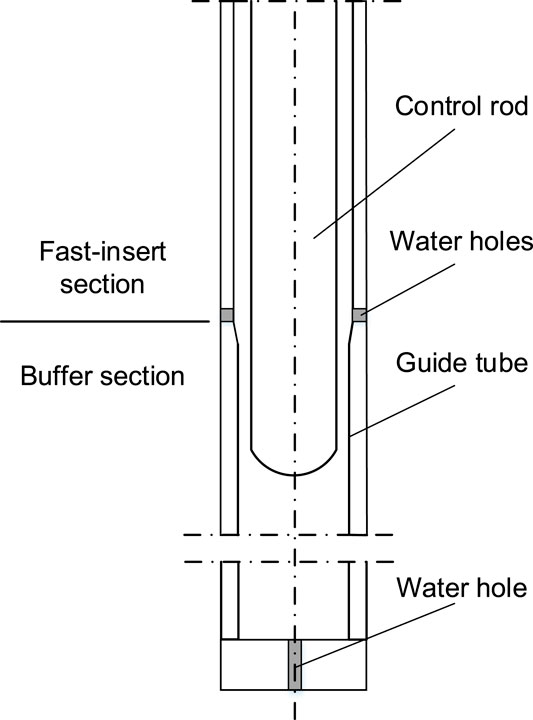
FIGURE 1. The geometry model of control rod mechanism.

The experiment selected in this article is designed for the dropping course of control rod assembly in some small reactors (Xiao et al., 2017). The control rod guide tube used in the experiment is shown in Figure 1, including the fast insertion section and buffer section, and flood holes are arranged at the bottom of the fast insertion section and the bottom of the guide tube convenient for the outflow of cooling water in the guide tube during rod dropping. The experiment studied the falling behavior of a single control rod in the guide tube. A high-speed camera was utilized to measure the displacement-time curve and speed-time curve of the control rod during the drop process, and a pressure sensor was utilized to measure the pressure-time curve in the guide tube. The size of the control rod was consistent with that of the reactor, and the weight of the single control rod is 4.2 kg, which is obtained by distributing equally the weight of the whole moving parts of the reactor (including control rod assemblies, lead screw components, and detachable and fitting components) to each control rod. Figure 1 shows the geometric model constructed according to the experimental section, and the specific structural parameters are shown in Table 1.

Mesh Generation

Different meshing methods are applied to the meshing geometric model, whose basic principle is to discrete the continuous domain and then numerically solve the discrete domain. Mesh can be divided into structured mesh, unstructured mesh, and hybrid mesh to meet the requirements of different regions. Since 1DOF equation solver is selected in this article to analyze and solve the dropping track of the control rod, the use of hexahedral mesh with dynamic mesh model is needed. But the computational domain belongs to typical long aspect ratio geometry whose dimension along the height is much larger than the radial dimension in which there are several complex local structures (flood holes and narrow gap), so it is very difficult to generate the structural hexahedron mesh in the whole geometry. Therefore, it is necessary to use hybrid mesh, which can combine the advantages of both structured and unstructured meshes. The computational domain is divided into dynamic fluid domain and static fluid domain. For the dynamic fluid domain, that is, the region involved in capturing the track of the control rod, the hexahedral mesh is selected; for the static fluid domain, both hexahedral mesh and tetrahedral mesh are used in order to control the number of meshes while ensuring the computational accuracy. At the same time, the meshes of the flood hole, drainage hole, narrow annular gap, and other small local places in the process were refined.

In dynamic mesh computing, the layering method is selected to update the mesh, which is suitable for 1DOF equation solver. It is noteworthy that this method has certain requirements on the mesh type near the moving boundary, which must be a quadrilateral (two-dimensional), triangular prism or hexahedral mesh. Due to the irregular geometric structure of the dynamic fluid domain, it is extremely difficult to completely generate triangular prisms or hexahedral meshes. Therefore, the whole dynamic fluid domain is divided into three segments along the flow direction, as shown in Figure 2. The part in the middle containing the head area of the control rod is an unstructured tetrahedral mesh, and the two ends of the dynamic fluid domain, that is, the computing domain adjacent to the moving boundary, are divided into hexahedral meshes.

FIGURE 2

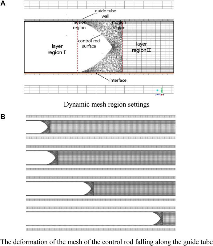
FIGURE 2. Control rod mesh settings: (A) dynamic mesh region settings; (B) the deformation of the mesh of the control rod falling along the guide tube.

When computational fluid dynamics (CFD) technique is applied to solve the computational model, the convergence of calculation and the correctness of simulation results depend on the type, quantity, and quality of the mesh. The errors of simulation and experiment mainly include the approximate error of calculation model, discrete error of numerical calculation area, iteration error generated by iteration times, and error generated by computer. In general, the finer the mesh, the smaller the dispersion error. However, when the mesh is further refined, the discrete points will increase and the rounding error is going to get bigger correspondingly. Therefore, the node number of mesh is not always “the more, the better”; what is more, too many nodes will also affect the computing efficiency and increase the computing cost, so it is necessary to find a balance between the accuracy, efficiency, and cost of the calculation in order to get the mesh that meets the requirements of the calculation. According to the previous steps of mesh generation, different mesh sizes were selected in turn to divide the mesh of the computing model, and the node number suitable for the computing model in this article was obtained through the analysis of mesh independence. In order to ensure the comparability of the calculation results, all the solution settings should remain the same except for the number of nodes in the calculation model; for example, the turbulence model, boundary conditions, solution methods, and residual accuracy are consistent in each calculation. The results of the mesh independence check carried out in this article are shown in Table 2. In the calculation, the process of the dropping of the control rod is emphasized, so the maximum velocity in the process is selected as the sensitive parameter for analysis.

TABLE 1

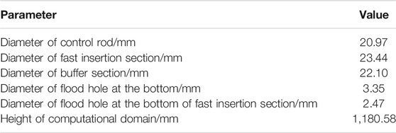
TABLE 1. Geometric model parameters.

TABLE 2

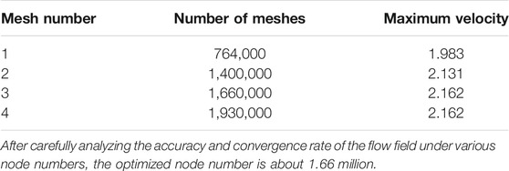
TABLE 2. Geometric model parameters.

After carefully analyzing the accuracy and convergence rate of the flow field under various node numbers, the optimized node number is about 1.66 million.

Boundary and Solution Settings

The experiment was carried out under normal pressure, with a pressure of 0.1 MPa and a temperature of 20°C. Under those conditions, the density of water was 998 kg/m³ and the kinematic viscosity 1.003 × 103 kg/(m²s). The boundary condition of the outlet of the fluid domain was set as the pressure outlet, and the gauge pressure was 0 Pa. The initial falling speed of the control rod assembly was set at 0 m/s. The shear condition of the solid wall was set to no slip and no penetration. The finite volume method was used to discretize the fluid computational control equations and transform the partial differential equations into algebraic equations, which are solved using the SIMPLE algorithm. The second-order upwind format was selected as the interpolation format of pressure and momentum, whereas the first-order upwind format was selected as the interpolation format of both turbulent kinetic energy and turbulent dissipation rate to improve the stability and speed up the calculation. The calculation convergence accuracy was set to 1 × 10^–3, when the residual curve reached this value, and the calculation was considered convergent.

For the dynamic mesh calculation, the layer method is selected to update the mesh. The generation and disappearance of the mesh are controlled by the splitting factor and merge factor. According to the default value in FLUENT, the splitting factor is set to 0.4 and the merge factor to 0.2: when the size of the mesh on the moving boundary is greater than (1 + 0.4) times the basic mesh size, one mesh will be split into two new meshes; when the size of the mesh on the moving boundary is smaller than 0.2 times the basic mesh size, two meshes will combine into one mesh. The control rod continuously moves downward under the action of gravity, and the mesh at the bottom of the control rod is continuously compressed and disappears, with the number of meshes decreasing. The laminated meshes at the top of the control rod are continuously stretched and divided into new meshes, and the number of meshes increases. Figure 2 (b) shows the mesh deformation in the dynamic fluid domain during rod dropping. Because the motion law of moving parts is unknown, 6DOF model is selected to solve the passive dynamic mesh problem. User-defined function (UDF) is compiled by C language to define the quality and force of the control rod.

Results and Analysis

In the experiment, the displacement-time curve and velocity-time curve in the process of rod dropping were measured by a high-speed camera, whereas the pressure-time curve of the guide tube was measured by using pressure sensors. However, because the location of the pressure sensor is not given in the reference, the simulation results cannot be extracted for comparison and verification. Therefore, this section intends to verify the correctness of the simulation results by comparing the speed-time curve and displacement curve of the control rods.

The calculated results of this article are in good agreement with the experimental data in terms of the trend; however, there are still some slight differences in the specific values. The experimental results tell that the control rod keeps accelerating in the initial stage of dropping, and the speed gradually declines when it reaches its maximum at about 2.0 m/s. In the initial stage of dropping, gravity is much greater than buoyancy and friction, the direction of acceleration is downward, and the control rod continues to accelerate. As the speed of the control rod increases gradually, the buoyancy and friction on the control rod increase correspondingly, the acceleration continues to decrease, and the speed of the control rod further increases. When the speed of the control rod increases to the maximum value, the acceleration becomes zero and the gravity, buoyancy, and friction forces reach a balance together. When the control rod moves further downward, the resultant upward forces of buoyancy and friction are greater than that of gravity and the speed of the control rod gradually decreases. After entering the buffer section, since the diameter of this section is smaller than that of fast insertion section, the friction force significantly increases, the vertical upward resultant force further increases same as that of acceleration, and the speed of the control rod decreases rapidly.

The numerical simulation of this article proposes the same trend with the experiment, but there are still slight differences in data. This is because the precise size of the experimental section is not given in the references. The geometric size used in the simulation is given by measuring the cloud picture of physical distribution from the literature.

Because the size of the simulation domain is very small (the distance between the control rod and the guide tube wall of the fast insertion section is less than 2 mm, and the distance between the pipe wall of the buffer section is less than 1 mm), small deviation between geometric structure and the experimental section will be reflected in the results. So numerical deviation between both is reasonable.

Figure 3 shows the comparison between the calculated displacement-time curve and velocity-time curve of the control rod and the experimental measurement. The control rod falls from the guide tube from the same height with an initial velocity of 0 m/s. Since the velocity-time curve obtained by the numerical simulation is consistent with the experimental measurement trend, the displacement-time curve trend of the control rod is in good agreement with the experimental measurement.

FIGURE 3

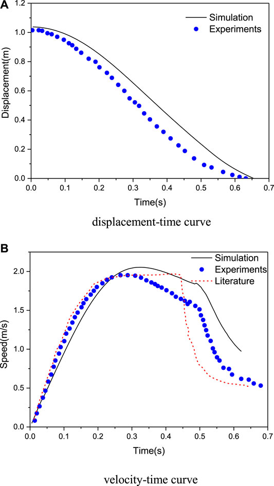
FIGURE 3. Comparison between simulation and experiments: (A) displacement–time curve; (B) velocity–time curve.

As the control rod continuously enters the guide tube to squeeze the fluid in the guide tube, the pressure in the guide tube continues to increase. When the control rod enters the buffer section, the four water holes on the sidewall of the guide tube are quickly covered and the annular gap between the control rod and the guide tube is also instantly reduced. The sudden change of the outflow area leads to a sharp increase in the pressure in the guide tube, which forms large pressure difference resistance at the bottom of the control rod. Under the action of this differential pressure resistance, the control rod assembly quickly decelerates; as the movement speed of the control rod decreases, the pressure in the guide tube decreases accordingly, as shown in Figure 4, which is the same as the changing trend of the guide tube measured by the pressure sensor in the experiment.

FIGURE 4

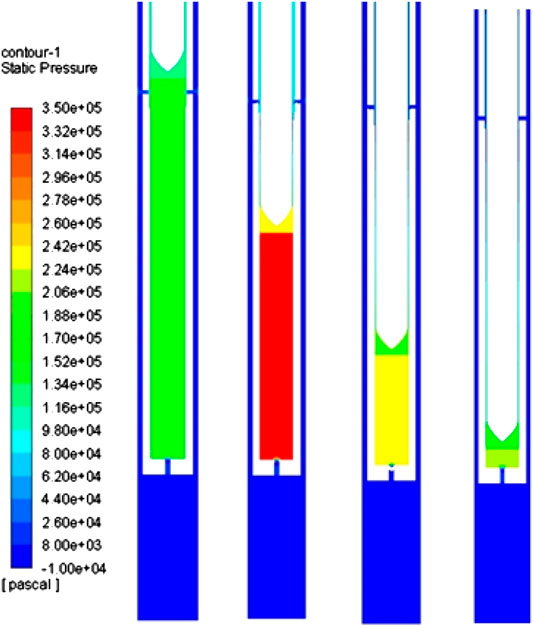
FIGURE 4. Pressure distribution of the guide tube during dropping.

The falling time of the control rod has always been a key parameter considered in the design of the driveline of the control rod. Through numerical simulation, it is calculated that the falling time of the control rod in the fast insertion section is 490 ms, the buffer time is 165 ms, and the maximum speed of the control rod is 2.16 m/s. Table 3 compares these key parameters in the experimental and numerical simulation results. Considering the difference between the numerical simulation geometry and the experimental section size, the error between the two is relatively small.

TABLE 3

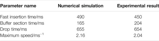
TABLE 3. Comparison of numerical simulation and experimental data.

Therefore, the comparative analysis in this section proves the correctness and accuracy of the simulation calculation. This method can be used to calculate important parameters such as control rod drop time and speed, which can provide a reference for the optimization design of the control rod driveline structure.

Conclusion

In this study, a three-dimensional fluid simulation model of a single control rod was established, and the falling behavior of the control rod was simulated and analyzed based on FLUENT dynamic mesh technology. Through simulation calculation, the displacement-time curve, velocity-time curve, and pressure-time curve of the single control rod drop and important parameters such as the drop time and impact of the control rod were obtained. The results of the simulation calculation were compared with the test results to verify the correctness and accuracy of the simulation calculation. This method can be used to calculate and predict important parameters such as control rod drop time and impact force so as to provide a reference for the optimal design of the control rod driveline structure.

Data Availability Statement

The raw data supporting the conclusions of this article will be made available by the authors, without undue reservation.

Author Contributions

JC wrote and presented this work; ZW provided technical support; CL, JZ, and SB provided the experiment data; and QF assisted with the manuscript writing.

Conflict of Interest

ZW works at one of the research departments in China Nuclear Power Engineering Co., Ltd. This work is concentrated on the verification of a numerical method for control rod drop. Both software or the research method applied in this paper has nothing to do with his company's business field. Also, this work doesn't receive any financial support from his company or anyone else.

The remaining authors declare that the research was conducted in the absence of any commercial or financial relationships that could be construed as a potential conflict of interest.

Glossary

ρ Fluid density, kg/m³
t Time, s
µ Viscosity, Pa·s
U Velocity vector, m/s
µ_eff Effective viscosity, Pa·s
µ_t Turbulent viscosity, Pa·s
P′ Pressure, Pa
S_M Sum of volumetric forces, N
V Volume, m³
ϕ Source phase
Γ Diffusion coefficient, m²/s
A_J Area of vector, m².

References

Chen, B., and Liu, C. (2007). Light water reactor fuel element. Beijing, China: chemical Industry Press.

Google Scholar

Collard, B. (1999). RCCA drop kinetics test, calculation, and analysis. Abnormal friction force evaluation. 7th International conference on nuclear engineering, April 19–23, 1999 (Tokyo, Japan: Japan Society of Mechanical Engineers), 4252.

Google Scholar

Peng, L., Tong, L., and Zhou, Y. (2013). Analysis of fluid-structure transverse coupling in the process of rod drop. Nucl. Technol. 36 (4), 82–86.

Google Scholar

Qu, P., Bo, Y., and Xie, Z. (2008). Numerical simulation of flow field of machine gun hydraulic buffer based on CFD. Equip. Manufact. Technol. 12, 58–60. doi:10.4028/www.scientific.net/AMR.588-589.1264

CrossRef Full Text | Google Scholar

Qu, T., and Chen, H. (2001). Analysis of falling time of control rods in nuclear power plant under strong earthquake. J. Comput. Mech. 18 (3), 364–370.

Google Scholar

Stabl, J., and Ren, M. (1999). Analytical modeling of control rod drop behavior. Transactions of the 15th international conference on structural mechanics in reactor technology, Seoul, Korea, August 15–20, 1999 (Korean Nuclear Society).

Google Scholar

Su, Y., Ji, D., and Zhang, J. (1977). Experimental report on hydraulic buffering of single control rod. Shanghai, China: Shanghai Nuclear Engineering Research and Design Institute.

Google Scholar

Sui, H. (2013). Proficient in CFD dynamic grid engineering simulation and case practice. Beijing, China: people's posts and Telecommunications Publishing House.

Google Scholar

Sun, L., Yu, J., and Yongtao, W. (2003). Calculation of falling time and course of control rod assembly. Nucl. Power Eng. 24 (1), 59–62.

Google Scholar

Xiao, C., Luo, Y., and Du, H. (2017). Simulation analysis of rod drop behavior of single control rod based on dynamic grid technology. Nucl. Power Eng. 38 (2), 103–107.

Google Scholar

Yoon, K. H., Kim, J. K., Lee, K. H., Lee, Y. H., and Kim, H. K. (2009). Control rod drop analysis by finite element method using fluid-structure inter-action for a pressurized water reactor power plant. Nucl. Eng. Des. 239 (10), 1857–1861. doi:10.1016/j.nucengdes.2009.05.023

CrossRef Full Text | Google Scholar

Yu, J., Yongtao, W., and Sun, L. (2001). Calculation of the resistance of the control rod assembly when it falls in the fluid environment. Nucl. Power Eng. 22 (3), 236–241.

Google Scholar