Productivity Prediction Model for Stimulated Reservoir Volume Fracturing in Tight Glutenite Reservoir Considering Fluid-Solid Coupling

At present, the main development mode of “horizontal well + volume fracturing” is adopted in a tight glutenite reservoir. Due to the existence of conglomerate, the seepage characteristics are more complex, and the production capacity after volume fracturing is difficult to predict. In order to solve this problem, a dual media unstable seepage model was established for matrix seepage and discrete fracture network seepage when considering the trigger pressure gradient. By considering the Poisson's ratio of stress sensitivity in an innovative way, the coupling model of permeability and stress is improved, and the production prediction model of volume fracturing horizontal well in a tight glutenite reservoir based on the fluid-solid coupling effect is formed. The finite element method is used to numerically solve the model, and the fitting verification of the model is carried out; the impact of stress sensitivity, producing pressure difference, fracture length, number of fracture clusters and fracture flow capacity conductivity on productivity is analyzed, which has certain guiding significance for the efficient development of volume fracturing in a tight glutenite reservoir.

Introduction

Horizontal well productivity prediction is very important in tight reservoir development. Especially for reservoirs with ultra-low permeability and tight reservoirs, unstable well-production systems may increase the difficulty of well production prediction (Ren et al., 2019; Zhang et al., 2019c). Friehauf et al. (2009) developed a new productivity prediction model that calculates the productivity of a hydraulically fractured well, taking into account the effect of damage of the fracture face from fluid leak-off. Results of the new productivity prediction model are compared with McGuire, Prats and Raymond models. The existing models assume either elliptical or radial flow around the well with permeability varying azimuthally. He found that there were significant differences in the calculated well productivity, which indicate that earlier assumptions made about the flow geometry lead to a serious overestimation of the well PI. The new productivity prediction model can be used to quickly calculate the productivity of wells that have both a finite-conductivity fracture and damage in the invaded zone. Considering the characteristics of unconventional oil and gas seepage, the trilinear flow model was first adopted in the study of volume fracturing horizontal well seepage. The pressure and production dynamics could be analyzed based on the trilinear analytical model, which was adopted by Brown et al. (2011). The two-hole three-region composite analytical model of volume fracturing horizontal wells was established by Brohi et al. (2011). The model described an oil reservoir in the inner region with dual porosity media, oil reservoir in the exterior region with single porosity media. The model was used for the study on tight gas reservoirs, shale gas reservoirs and tight oil reservoirs. Sennhauser et al. (2011) established the multistage fracturing horizontal well productivity model. The model can accurately describe the reservoir in terms of geology, fluid characteristics and pressure profile. It is also demonstrated that the overall productivity of multistage fracturing horizontal wells is determined by a number of parameters, including well spacing, fracture spacing, fracture size and characteristics, and the location of the first and last fractures. The model was applied to the study of tight gas reservoirs, shale gas reservoirs and tight oil reservoirs. Based on the seepage characteristics of porous media in unconventional reservoirs and geological data. Na Zhang and Abushaikha (2019) presented a new fully-implicit mimetic finite difference method (FDM) to simulate reservoir fluid flow. It had been applied to many fields due to its local conservativeness and applicability of any shape of polygon. The principle of the MFD method and the corresponding numerical formula for discrete fracture model are described in detail. The new fully-implicit mimetic finite difference method is tested through some examples to show the accuracy and robustness and the model can be used to predict the well production. Jackson et al. (2013) presented a new approach to simulate fluid flow by adopting Control-Volume-Finite-Element Method (CVFM). The new approach disposes of the pillar-grid concept that has persisted since reservoir simulation began. The new approach promotes the representation of multi-scale geological heterogeneity and the prediction of flow through that heterogeneity significantly. Multiphase flow is simulated using a novel mixed finite element formulation centered on a new family of tetrahedral element types, PN(DG) − PN + 1, which has a discontinuous Nth-order polynomial representation for velocity and a continuous (order N + 1) representation for pressure. The new approach preserves key flow features associated with realistic geological features that are usually lost. Li and Li. (2012) derived a new production prediction model theoretically with the pressure sensitivity of permeability being considered, and used the production data from a low permeability oil field to test and verify the model. The pressure sensitivity coefficient of permeability has been calculated by using the new model with the field data. He founded that the permeability near the well bottom decreased significantly because of the drop in pressure in low permeability reservoirs. An obvious permeability decline funnel could be formed even if the formation was homogeneous before development It was found that the productivity index is no longer a constant in low permeability reservoirs with serious pressure sensitivity of permeability. The pressure sensitivity of permeability should be considered when low permeability reservoirs are being developed. Otherwise, the production will be greatly overestimated. Doe et al. (2013) carried out discretization of complex fracture network in the fractured region, established the productivity model of multiple porosity media, and calculated the contribution rate of natural fractures in the productivity. Cao et al. (2015) established a full analytical mathematical productivity model considering friction, and compared and analyzed the difference between the analytical method and the finite-difference solution results, proving that the model is more accurate in spatial discretization and other aspects (Johansen et al., 2015). Taking the tight reservoir of Daqing Oilfield as the study object, Hu et al. (2017) established a numerical model of production capacity based on the theory of unsteady seepage mechanics and superposition principle, which was used to calculate and analyze the production capacity of fracturing horizontal wells. Yang et al. (2019) and Zhang et al. (2019a) established the productivity model of the shale reservoir to optimize the fracture spacing, considering the linear flow in the reservoir and the linear flow coupling model in hydraulic fractures, and proved that the productivity of multi-fracture horizontal wells are inversely proportional to the fracture spacing. The maximum capacity after volume fracturing can be achieved by reducing the fracture spacing. The production capacity of the production well can be doubled by reducing the cluster spacing from 70 to 15 ft.

Compared with the Poisson’s ratio of conventional tight sandstone, the Poisson’s ratio of tight glutenite reservoir, a mechanic parameter of stone, is greatly different. In this paper, a productivity prediction model for volume fracturing horizontal well considering fluid-solid coupling was established, combining the principle of effective stress and constitutive relation of rock skeleton, while fully taking into account the fluid-solid coupling effect of the tight reservoir; the impact of Poisson’s ratio of stress sensitivity and lithological characteristic parameters on the fluid-solid coupling effect was considered in an innovative manner, and a fluid-solid full coupling productivity model suitable for the characteristics of glutenite oil reservoir was established. The accuracy and reliability of the model was validated by comparing the mathematical model of stress field and seepage field of volume fracturing horizontal well in a tight reservoir with the actual production well (Zhang et al., 2019b).

Establishment of Productivity Prediction Model

Seepage Field Model of Volume Fracturing Horizontal Well in Tight Reservoir

Geometric Model of Volume Fracturing Horizontal Well

In the “Five-region Model” proposed by Stalgorova and Mattar. (2012), and the “Composite Flow Model” proposed by Su Yuliang et al., it is believed that the main fracture and natural fracture are formed by fracturing form complex fracture clusters after volume fracturing of horizontal wells, and there are non-fractured regions between the clusters. The reservoir area of volume fracturing horizontal wells are composed of three parts: reservoir matrix, natural fracture (unmodified) region, artificial fracture and natural fracture interlaced fracture network region. Based on the above conclusions, a volume fracturing horizontal well model for a tight glutenite reservoir is established, as shown in Figure 1.

FIGURE 1

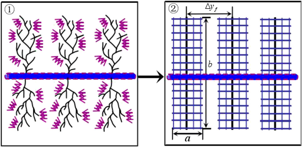
FIGURE 1. Schematic diagram of geometric model.

The formation and fluid meet the following conditions: 1) thickness of the reservoir is h, with outer boundary closed, and with natural fracture; 2) rocks and fluids are slightly compressible; 3) the impact of gravity and temperature changes are not considered for the seepage process.

Mathematical Model for Seepage of Volume Fracturing Horizontal Well

Mathematical Model for Seepage of Matrix—Natural Fracture System

The fluid motion equation in a matrix system considering the trigger pressure gradient:

$v_m=-\frac{K_m}{\mu }\left(\nabla P_m-\lambda \right)(1)$

Equation for state of rock skeleton and fluid in matrix system

$\varphi ={\varphi }_{\text{0}}{e}^{-C_P\left(P_i-P_m\right)},\rho ={\rho }_0{e}^{-C_L\left(P_i-P_m\right)}(2)$

Equation for continuity of a single phase compressible fluid

$\nabla \left(\rho v_m\right)+Q_m=-\frac{\partial \left(\rho \varphi \right)}{\partial t}(3)$

Eqs (1) and (2) were substituted into the continuity Eq. (3):

${\nabla }^2{P}_m+C_L{\left(\nabla P_m\right)}^2-\lambda C_L\nabla P_m-\frac{\varphi \mu C_{\text{m}}}{K_m}\frac{\partial P_m}{\partial t}-\alpha \left(P_m-P_n\right)=0(4)$

$C_{\text{m}}=C_P+C_L(5)$

Since the $\nabla P_m$ is very small, Eq. (3) can be reduced to the following equation.

${\nabla }^2{P}_m-\lambda C_L\nabla P_m-\frac{{\varphi }_{\text{m}}\mu C_{\text{m}}}{K_m}\frac{\partial P_m}{\partial t}-\alpha \left(P_m-P_n\right)=0(6)$

Eq. (6) is the equation for the seepage governing differential of single-phase micro-compressible fluid in bedrock when the trigger pressure gradient is considered. Similarly, the governing differential equation of the natural fracture system can be obtained as follows.

${\nabla }^2{P}_n-\frac{{\varphi }_{\text{m}}\mu C_{\text{m}}}{K_m}\frac{\partial P_m}{\partial t}+\alpha \frac{K_m}{K_n}\left(P_m-P_n\right)=0(7)$

The initial and boundary conditions:

$\{\begin{array}{l}{P}_m\left(x,y,z,t=0\right)=P_n\left(x,y,z,t=0\right)=P_i\\ P_n\left(x,y,z,t\right)=P_f\left(x,y,z,t\right)\\ {\frac{\partial P_m}{\partial x}|}_{x=x_e}={\frac{\partial P_m}{\partial y}|}_{y=y_e}={\frac{\partial P_m}{\partial z}|}_{z=z_e}\\ {\frac{\partial P_n}{\partial x}|}_{x=x_e}={\frac{\partial P_n}{\partial y}|}_{y=y_e}={\frac{\partial P_n}{\partial z}|}_{z=z_e}=0\end{array}(8)$

Seepage Model of Fracture Network System

The fluid motion equation:

$v_f=-\frac{K_f}{\mu }{P}_f(9)$

The equation for state:

${\varphi }_{\text{f}}={\varphi }_{\text{fo}}{e}^{-C_{\text{o}}\left(P_i-P_f\right)},\rho ={\rho }_0{e}^{-C_L\left(P_i-P_m\right)}(10)$

The equation for continuity

$\nabla \left(\rho v_f\right)-Q_f=\frac{\partial \left(\rho {\varphi }_{\text{f}}\right)}{\partial t}(11)$

Similarly, the seepage governing differential equation:

${\nabla }^2{P}_f-\frac{{\varphi }_f\mu C_{\text{f}}}{K_f}\frac{\partial P_f}{\partial t}=0(12)$

The initial and boundary conditions

$\{\begin{array}{l}{P}_f\left(x,y,z,t=0\right)=P_i\\ P_f\left(x,y,z,t\right)=P_m\left(x,y,z,t\right)=P_n\left(x,y,z,t\right)\end{array}(13)$

Definite Conditions for Solution of Seepage Field

In order to solve the nonlinear equations, some fixed value conditions are set. These conditions are definite conditions. For example, the fixed pressure condition is that the well is produced under a certain flow pressure. For the mathematical model for the seepage field of volume fracturing horizontal wells in tight reservoirs, the definite conditions mainly include the initial formation pressure conditions, the definite pressure production.

Initial conditions:

$p_m\left(x,y,z,t=0\right)=p_n\left(x,y,z,t=0\right)=p_f\left(x,y,z,t=0\right)=p_i(14)$

Boundary conditions:

${p|}_{r=r_w}=p_w(15)$

Model for Stress Field of Volume Fracturing Horizontal Well in Tight Reservoir

Assumptions: 1) The rock is the deformation of porous media; 2) The rock particles are incompressible, while particle pores can be compressed; 3) The impact of temperature change on rock deformation is not considered; 4) Rock deformation is a small elastoplastic deformation; 5) The compression coefficient of pore changes (Jianjun et al., 2002; Liu et al., 2018; Zhao and Du, 2019).

Equation for Constitutive Relation

$d{\sigma }_{ij}=D_{ijkl}d{\epsilon }_{kl}(16)$

Geometric Equation

${\epsilon }_{ij}=\frac{1}{2}\left(u_{i,j}+u_{ji}\right)(17)$

Differential Equation for Stress Equilibrium

Before the reservoir is developed, any unit (infinitely small) in the reservoir is in static equilibrium. When the reservoir is developed, the pore pressure of the reservoir will change. Meanwhile the effective stress also changes. This change can be expressed by the stress equilibrium differential equation. A hexahedral differential element is used to represent the stress state in the space, as shown in Figure 2 and the length of each side is dx, dy, dz respectively.

FIGURE 2

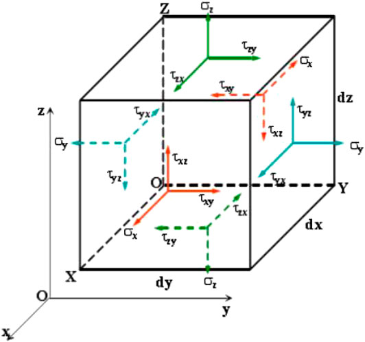
FIGURE 2. Schematic diagram for stress state of the element in the space.

The equilibrium equation of the element in the x direction:

$\begin{array}{l}\left({\sigma }_{\text{x}}+\frac{\partial {\sigma }_{\text{x}}}{\partial x}\right)dydz-{\sigma }_{\text{x}}dydz+\left({\tau }_{\text{xy}}+\frac{\partial {\tau }_{\text{xy}}}{\partial y}\right)dzdx-{\tau }_{\text{xy}}dzdx\\ +\left({\tau }_{\text{xz}}+\frac{\partial {\tau }_{\text{xz}}}{\partial z}\right)dxdy-{\tau }_{\text{xz}}dxdy+f_{x}dxdydz=\text{0}\end{array}(18)$

So if we simplify Eq. (18), we get Eq. (19).

$\frac{\partial {\sigma }_{\text{x}}}{\partial x}+\frac{\partial {\tau }_{\text{xy}}}{\partial y}+\frac{\partial {\tau }_{\text{xz}}}{\partial z}+f_x=\text{0}(19)$

Similarly, the differential equation for equilibrium in the y and z directions:

$\frac{\partial {\sigma }_{\text{y}}}{\partial y}+\frac{\partial {\tau }_{\text{xy}}}{\partial x}+\frac{\partial {\tau }_{\text{yz}}}{\partial z}+f_y=\text{0}(20)$

$\frac{\partial {\sigma }_{\text{z}}}{\partial z}+\frac{\partial {\tau }_{\text{xz}}}{\partial x}+\frac{\partial {\tau }_{\text{xz}}}{\partial y}+f_z=\text{0}(21)$

Definite Conditions for Solution of Stress Field

For the mathematical model for stress field of horizontal well in a tight reservoir, its definite conditions can be divided into initial conditions and boundary conditions, and the boundary conditions can be divided into stress boundary conditions and displacement boundary conditions (Zhang et al., 2018). The initial conditions for the stress field are consistent with those for the model for seepage field.

Stress field displacement boundary conditions:

${u|}_{{\Omega }_e}=\overline{u}(22)$

Stress field stress boundary conditions:

${{\sigma }_{\text{ij}}\cdot n|}_{{\Omega }_e}=\overline{T_i}(23)$

Dynamic Cross Coupling Model of Seepage Field and Stress Field

Permeability Coupling Relationship

Yin et al. (2019) studied the permeability coupling of tight glutenite reservoirs by considering the influence of young’s modulus and initial permeability comprehensively. However, he did not consider the influence of Poisson’s ratio which is a rock characteristic parameter. Young’s modulus can reflect the changing relationship of longitudinal strain stress. Compared with Young’s modulus, Poisson’s ratio reflects the longitudinal and transverse strain ratio and better reflects the overall strain of the rock. In this paper, the initial permeability, Young’s modulus and Poisson’s ratio are considered.

$\alpha =c_1{\alpha }_E+c_2{\alpha }_k+c_3{\alpha }_{\upsilon }(24)$

${\alpha }_E=1.465-0.3553\ln E(25)$

${\alpha }_K=0.4834K_0^{-0.3422}(26)$

${\alpha }_{\upsilon }=\ln \upsilon (27)$

Substitute the data into Eqs 24-27:

$K_{\text{f}}=K_{f0}\exp \left[-\mathrm{0}\mathrm{.087}\left({\sigma }_n-p\right)\right]$

Coupling Relation of Porosity

Ran and Li. (1997) derived the porosity strain model through the definition of porosity. The volumetric strain parameters themselves imply the mechanical properties of rocks, and the derived porosity coupling model is as follows:

$\varphi =\frac{{\varphi }_0+{\epsilon }_v}{1+{\epsilon }_v}(28)$

Solution of Productivity Prediction Model

Finite Element Solution of Seepage Model

The whole reservoir is considered as a continuous calculation domain, including porous media seepage considering the trigger pressure gradient and the fracture network seepage of the volume fracturing region, and fracture fluid flow within the volume fracture system (Zhang et al., 2020). For fracture fluid seepage in the fracture network system, the actual a three-dimensional fracture is equivalent to two-dimensional fracture with certain fracture openness with a discrete fracture network model. So, the whole calculation domain governing equation ${\Omega }_{i,m}$ of three-dimensional integral form can be reduced as.

${\displaystyle \underset{\Omega }{\iiint }Fd\Omega }={\displaystyle \underset{{\Omega }_{f\left(3D\right)}}{\iiint }Fd{\Omega }_f}+{\displaystyle \underset{{\Omega }_{m,n\left(3D\right)}}{\iiint }Fd{\Omega }_{m,n}}={\displaystyle \underset{{\Omega }_{f\left(2D\right)}}{\iint }Fd{\Omega }_f}+{\displaystyle \underset{{\Omega }_{m,n\left(3D\right)}}{\iiint }Fd{\Omega }_{m,n}}(29)$

The approximate expression of the pressure field function is obtained by taking any element in the system:

$P_{\text{m}}\approx P_{i,m}{N}_{i,m}(30)$

Eq. (30) is substituted into Eq. (6) to obtain the expression of characteristic matrix of element ${\Omega }_{i,m}$

$\begin{array}{l}{\displaystyle \underset{{\Omega }_{i,mn}}{\iiint }\left(\nabla N_{i,mn}^T\nabla N_{i,mn}+\lambda \nabla N_{i,mn}^T\nabla N_{i,mn}\right)d{\Omega }_{i,mn}}{P}_{i,m}+\left(1-{\omega }_n\right){\displaystyle \underset{{\Omega }_{i,mn}}{\iiint }{N}_{i,mn}^T\nabla N_{i,mn}d{\Omega }_{i,mn}}\frac{\partial P_{i,m}}{\partial t}{P}_{i,m}\\ +\alpha {\displaystyle \underset{{\Omega }_{i,mn}}{\iiint }{N}_{i,mn}\left(P_{i,m}-P_{i,n}\right)N_{i,mn}^{T}d{\Omega }_{i,mn}}=0\end{array}(31)$

Similarly, the element characteristic matrix expression of natural fracture seepage model ${\Omega }_{i,n}$:

$\begin{array}{l}{\displaystyle \underset{{\Omega }_{i,mn}}{\iiint }\nabla N_{i,mn}^T\nabla N_{i,mn}d{\Omega }_{i,mn}{P}_{i,m}+{\omega }_n{\displaystyle \underset{{\Omega }_{i,mn}}{\iiint }{N}_{i,mn}^T{N}_{i,mn}d{\Omega }_{i,mn}}\frac{\partial P_{i,m}}{\partial t}}-\alpha {\displaystyle \underset{{\Omega }_{i,mn}}{\iiint }{N}_{i,mn}\left(P_{i,m}-P_{i,n}\right)N_{i,mn}^{T}d{\Omega }_{i,mn}}\\ =2\pi h{\displaystyle \underset{{\Omega }_{i,m}}{\iiint }{q}_n}{N}_{i,mn}^{T}d{\Omega }_{i,mn}\end{array}(32)$

The element characteristic matrix expression of network fracture seepage ${\Omega }_{i,f}$ in volume fracturing region:

$\begin{array}{l}{\displaystyle K_{\mathrm{f}}\underset{{\Omega }_{\mathrm{i},\mathrm{f}}}{\iint }\nabla N_{i,f}^T\nabla N_{i,f}d{\Omega }_{i,f}{P}_{i,f}+{\omega }_f{K}_{\mathrm{f}}{\displaystyle \underset{{\Omega }_{\mathrm{i},\mathrm{f}}}{\iint }{N}_{i,f}^T{N}_{i,f}d{\Omega }_{i,f}}\frac{\partial P_{i,f}}{\partial t}}\\ =2\pi h{\displaystyle \underset{{\Omega }_{\mathrm{i},\mathrm{f}}}{\iint }{q}_f}{N}_{i,f}^{T}d{\Omega }_{i,f}\end{array}(33)$

Assuming that the initial reservoir flow occurs in the natural fracture system ${\Omega }_{\text{i},n}$and flows into the fracture network system ${\Omega }_{i,f}$, the solution can be obtained by the implicit backward difference scheme, and finite element closed equations with unknown quantities in the next time step ${\Omega }_{i,f}$ can be obtained:

$\begin{array}{l}\left\{{\displaystyle \underset{{\Omega }_{i,mn}}{\iiint }\nabla N_{i,mn}^T\nabla N_{i,mn}d{\Omega }_{i,mn}+K_f{\displaystyle \underset{{\Omega }_{i,f}}{\iint }\nabla N_{i,f}^T\nabla N_{i,f}d{\Omega }_{i,f}}}\right\}{P}_n^{k+1}\\ +\frac{{\omega }_n{\displaystyle \underset{{\Omega }_{i,mn}}{\iiint }{N}_{i,mn}^T{N}_{i,mn}d{\Omega }_{i,mn}+{\omega }_f{K}_f{\displaystyle \underset{{\Omega }_{i,f}}{\iint }{N}_{i,f}^T{N}_{i,f}d{\Omega }_{i,f}}}}{t^{k+1}-t^k}{P}_n^{k+1}\\ +\alpha {\displaystyle \underset{{\Omega }_{i,mn}}{\iiint }{N}_{i,mn}{N}_{i,mn}^{T}d{\Omega }_{i,mn}}{P}_n^{k+1}\\ =Q_n^{k+1}+\frac{{\omega }_n{\displaystyle \underset{{\Omega }_{i,mn}}{\iiint }{N}_{i,mn}^T{N}_{i,mn}d{\Omega }_{i,mn}+{\omega }_f{K}_f{\displaystyle \underset{{\Omega }_{i,f}}{\iint }{N}_{i,f}^T{N}_{i,f}d{\Omega }_{i,f}}}}{t^{k+1}-t^k}{P}_n^k\\ +\alpha {\displaystyle \underset{{\Omega }_{i,mn}}{\iiint }{N}_{i,mn}{N}_{i,mn}^{T}d{\Omega }_{i,mn}}{P}_m^k\end{array}(34)$

The pressure at the next time step of the matrix system is calculated according to the matrix natural fracture equilibrium equation of the entire reservoir:

$\begin{array}{l}\left\{{\displaystyle \underset{{\Omega }_{i,mn}}{\iiint }\left(\nabla N_{i,mn}^T\nabla N_{i,mn}+\lambda \nabla N_{i,mn}^T\nabla N_{i,mn}\right)d{\Omega }_{i,mn}+K_f{\displaystyle \underset{{\Omega }_{i,f}}{\iint }\nabla N_{i,f}^T\nabla N_{i,f}d{\Omega }_{i,f}}}\right\}{P}_m^{k+1}\\ +\frac{\left(1-{\omega }_n\right){\displaystyle \underset{{\Omega }_{i,mn}}{\iiint }{N}_{i,mn}^T{N}_{i,mn}d{\Omega }_{i,mn}+{\omega }_f{K}_f{\displaystyle \underset{{\Omega }_{i,f}}{\iint }{N}_{i,f}^T{N}_{i,f}d{\Omega }_{i,f}}}}{t^{k+1}-t^k}{P}_m^{k+1}\\ +\alpha {\displaystyle \underset{{\Omega }_{i,mn}}{\iiint }{N}_{i,mn}{N}_{i,mn}^{T}d{\Omega }_{i,mn}}{P}_m^{k+1}\\ =\frac{\left(1-{\omega }_n\right){\displaystyle \underset{{\Omega }_{i,mn}}{\iiint }{N}_{i,mn}^T{N}_{i,mn}d{\Omega }_{i,mn}+{\omega }_f{K}_f{\displaystyle \underset{{\Omega }_{i,f}}{\iint }{N}_{i,f}^T{N}_{i,f}d{\Omega }_{i,f}}}}{t^{k+1}-t^k}{P}_m^k\\ +\alpha {\displaystyle \underset{{\Omega }_{i,mn}}{\iiint }{N}_{i,mn}{N}_{i,mn}^{T}d{\Omega }_{i,mn}}{P}_n^k\end{array}(35)$

The whole continuous calculation domain can be solved through Eqs (34) and (35).

Finite Element Solution for Fluid-Solid Coupling Productivity Model

Differential equation for stress field:

$A\left(U\right)=0,\forall x\in \Omega (36)$

Boundary conditions:

$B\left(U\right)=0,\forall x\in \Gamma (37)$

The unknown function U is the field function that needs to be solved. A and B in Eqs (36) and (37) are differential operators for independent variables such as spatial coordinates and time. The equivalent integral form of differential Eq. (36) and boundary conditions Eq. (37) can be written by the Galerkin equation as follows:

${\displaystyle {\int }_{\Omega }{\text{v}}^T}A\left(U\right)d\Omega +{\displaystyle {\int }_{\Gamma }{\text{v}}^T}B\left(U\right)d\Gamma =0(38)$

According to the principle of effective stress, the total stress of reservoir rock is composed of effective stress and pore fluid pressure:

$\sigma ={\sigma }^{\prime }+\text{mp}(39)$

${\text{m}}^T=\left[111000\right](40)$

It is assumed that the displacement vector at any point in the calculation domain satisfies the following equation:

$U^T=\left[\text{u},v,w\right](41)$

The above equation can be expressed as:

$u=\left[{\text{IN}}_i,I{N}_j,I{N}_m,I{N}_p\right]a^{\prime }=N{a}^{\prime }(42)$

The following equation can be obtained by the combination of Eqs (17) and (41):

$\epsilon =B{a}^{\prime }=\left[B_i,B_j,B_m,B_p\right]a^{\prime }(43)$

$B_i=\left[\begin{array}{ccc}\frac{\partial N_i}{\partial x}& 0& 0\\ 0& \frac{\partial N_i}{\partial y}& 0\\ 0& 0& \frac{\partial N_i}{\partial z}\\ \frac{\partial N_i}{\partial y}& \frac{\partial N_i}{\partial z}& 0\\ 0& \frac{\partial N_i}{\partial z}& \frac{\partial N_i}{\partial y}\\ \frac{\partial N_i}{\partial z}& 0& \frac{\partial N_i}{\partial x}\end{array}\right](44)$

By substituting Eqs (19)-(23) and Eq. (36) into Eq. (38), the following equation can be obtained:

${\displaystyle {\int }_{\Omega }\delta {\text{u}}_i\left({\sigma }_{\text{ij},j}+f_i-\rho u_i\right)\text{d}\Omega -}{\displaystyle {\int }_{\Gamma }\delta u_i\left({\sigma }_{ij}{n}_j-\overline{T_i}\right)}d\Gamma =0(45)$

The above equation is integrated by parts and substituted into Eq. (42), Eq. (17) and the elastic constitutive matrix of rock to obtain the overall equilibrium equation of the fluid-solid fully coupled stress field:

$M\frac{d\overline{u}}{dt}+C\frac{d\overline{u}}{dt}+{\displaystyle \sum _e{\displaystyle {\int }_{{\Omega }_e}{B}^T\sigma d{\Omega }_e}}=F_{\Gamma }(46)$

$M={\displaystyle \sum _{\text{e}}{\displaystyle {\int }_{{\Omega }_e}\rho N^{T}N\text{d}\Omega ,C=}}{\displaystyle \sum _{\text{e}}{\displaystyle {\int }_{{\Omega }_e}\mu N^{T}N\text{d}\Omega }}{F}_{\Gamma }={\displaystyle \sum _{\text{e}}{\displaystyle {\int }_{{\Omega }_e}{N}^T\text{fd}\Omega +}}{\displaystyle \sum _{\text{e}}{\displaystyle {\int }_{{\Gamma }_e}{N}^T\overline{\text{T}}\text{d}\Gamma }}(47)$

The Galerkin weighted residual method is applied to the seepage field model and the following equations can be obtained:

$K_{\text{p}}^{T}a+Sp+Hp=F_f(48)$

$K_{\text{p}}={\displaystyle \sum _e\left({\displaystyle {\int }_{{\Omega }_e}{B}^{T}m{N}_{p}d{\Omega }_e}\right)}(49)$

$S={\displaystyle \sum _{\text{e}}{\displaystyle {\int }_{{\Omega }_e}{N}_{\text{p}}^T\frac{1}{Q}\text{d}{\Omega }_e,H=}}{\displaystyle \sum _{\text{e}}{\displaystyle {\int }_{{\Omega }_e}{\left(\nabla N_p\right)}^{T}k\nabla N_p\text{d}{\Omega }_e}}(50)$

To sum up, the matrix form of the equilibrium equations for the fluid-solid coupling mathematical model of porous media based on the full-coupling finite element method can be obtained as follows:

$\left[\begin{array}{cc}M& 0\\ 0& 0\end{array}\right]\left[\begin{array}{c}\overline{u}\\ P\end{array}\right]+\left[\begin{array}{cc}C& 0\\ K_p^T& S\end{array}\right]\left[\begin{array}{c}\overline{u}\\ P\end{array}\right]+\left[\begin{array}{cc}K& -K\\ 0& H\end{array}\right]\left[\begin{array}{c}\overline{u}\\ P\end{array}\right]=\left[\begin{array}{c}{F}_{\Gamma }\\ F_f\end{array}\right](51)$

Eq. (51) is substituted into COMSOL and the result is obtained.

Example for Calculation of Productivity Prediction Model

Comparison of Actual and Model Production

After establishing and solving the fluid-solid coupling model, the required parameters of the model are input into COMSOL (Table 1). Then the trend of the model simulated oil rate is obtained by using the full coupling of finite elements. Combined with the actual oil rate changes of production well, the trend of model simulated oil rate can be analyzed as shown in Figure 3. It can be seen from Figure 3 that the fitting error between the actual daily production and the simulation result of fluid-solid coupling model is small.

FIGURE 3

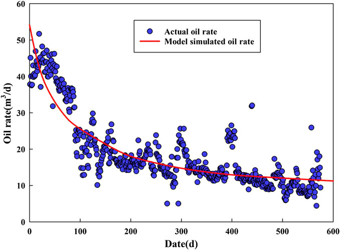
FIGURE 3. Comparison between actual production and model production.

Pressure Distribution of Model

Figures 4-6 show the variation of pore pressure around the well with production time. Figures 46 show the pressure distribution at 0, 300 and 600 days of production, respectively. As can be seen from the Figures, formation pressure gradually decreases in the horizontal well simulation production process, and the pressure change range is as follows: area near the wellbore of horizontal well ≥ volume fracturing region ≥ unmodified region of matrix. Globally, the reservoir fluid flow first occurs around the wellbore with a fast flow speed. After the fluid flows away, the supply fluid of the volume fracturing region and matrix flows into the wellbore from the fracturing region and matrix flow into the wellbore. The fluid of the entire formation flows around the wellbore of the horizontal well elliptically.

FIGURE 4

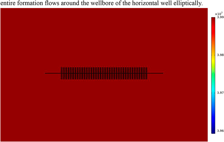
FIGURE 4. Formation pressure distribution in volume fracturing horizontal well (0 days).

FIGURE 5

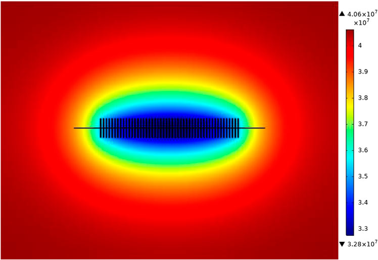
FIGURE 5. Formation pressure distribution in volume fracturing horizontal well (300 days).

FIGURE 6

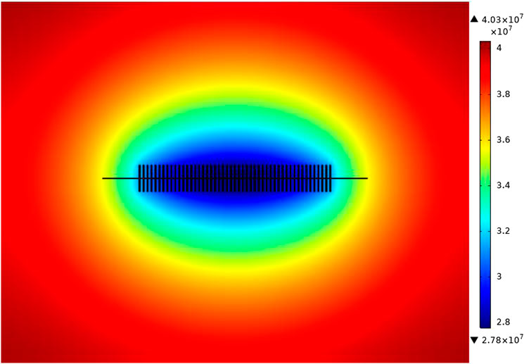
FIGURE 6. Formation pressure distribution in volume fracturing horizontal well (600 days).

Sensitivity Analysis

By sensitivity analysis of different parameters, the impact of each factor on production can be understood. These parameters mainly include stress sensitivity, producing pressure, fracture half length, number of fracture clusters and fracture flow capacity.

Stress Sensitivity

The fluid-solid coupling effect is mainly due to the change of reservoir pressure in the production process, which leads to the change of pore and permeability. And the change of permeability is obvious. Based on the rock mechanics characteristics of the glutenite, the stress sensitivity coefficient is a parameter to reflect the influence of stress change on permeability. The flow pressure is set to 26 MPa and other parameters remained unchanged by single factor analysis. The variation of the oil rate under different stress sensitivity coefficients is simulated.

As can be seen from Figures 7, 8, with the increase of the stress sensitivity coefficient, the production of the horizontal well is reduced. Under the effect of stress, the initial permeability of the reservoir, especially the volume fracturing region, is high, and the permeability loss with the change of stress is large, resulting in the decrease of production. In the actual production process, the control of the producing pressure should be considered to reduce the fluid-solid coupling effect on the productivity.

FIGURE 7

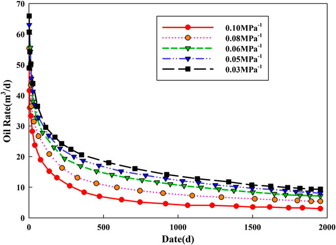
FIGURE 7. Daily oil production curve of different stress sensitivity coefficient.

FIGURE 8

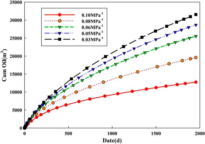
FIGURE 8. Cumulative oil production curve of different stress sensitivity coefficient.

Producing Pressure Difference

The change of pressure in the production process will also lead to the change of pore and permeability of reservoir. The fluid-solid coupling can be reflected by controlling the producing pressure difference of the model. The stress sensitivity coefficient is set to 0.06 MPa⁻¹ and other parameters remained unchanged by single factor analysis. The variation of oil rate under varying producing pressure differences is simulated.

As can be seen from Figures 9, 10, the daily production of volume fracturing horizontal well increases with the increase of producing pressure difference. The increase of producing pressure difference leads to a large drop in formation pressure, which will obviously affect the loss of formation porosity and permeability. Increasing the producing pressure difference will increase the cumulative production of the horizontal well, but the increasing rate will decrease. After increasing the producing pressure difference, the reservoir's available range increases, leading to higher production. However, it also enhances the fluid-solid coupling effect, resulting in a decrease in fluid flow capacity, which has some impact on the actual production of the horizontal well.

FIGURE 9

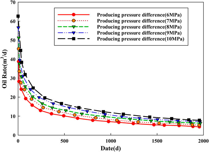
FIGURE 9. Daily oil production curve of different producing pressure difference.

FIGURE 10

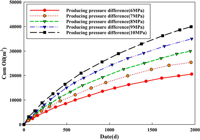
FIGURE 10. Cumulative oil production curve of different producing pressure difference.

Fracture Half Length

Fracture half length is one of the important parameters to control the area of SRV zone. By extending the fracture half length, the SRV zone of the reservoir can be expanded effectively. Therefore, fracture half-length has a great influence on horizontal well production. The variation of the oil rate under different fracture half lengths is simulated by single factor analysis.

As can be seen from Figures 11, 12, the increase of fracture half length has a small impact on the early productivity of the horizontal well. With the increase of fracture half-length, the growth trend of cumulative production is obvious. However, although the fracture half-length increases in a linear manner, the growth rate of cumulative production decreases to some extent. At the same time, considering the economic cost of on-site fracturing, there is some room for optimization of fracture half-length.

FIGURE 11

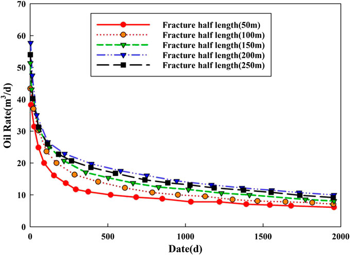
FIGURE 11. Daily oil production curve of different fracture half length.

FIGURE 12

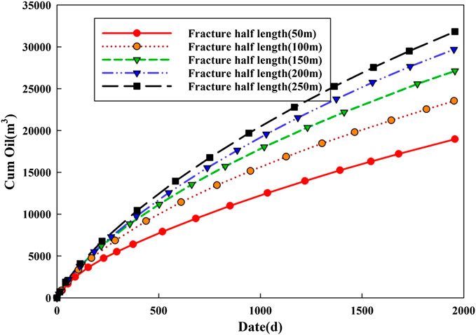
FIGURE 12. Cumulative oil production curve of different fracture half-lengths.

Number of Fracture Clusters

The number of fracture clusters could control the area of SRV zone. Therefore, the number of fracture clusters has a great influence on horizontal well production. The variation of oil the rate under different numbers of fracture clusters is simulated by single factor analysis.

As can be seen from Figures 13, 14, with the increase of fracture clusters, the growth trend of cumulative production is obvious. The increasing of fracture clusters has a great impact on the production of the horizontal well in the early stage and a small impact in the later stage. In the early production of the horizontal well, the oil supply is mainly from the volume fracturing region to the horizontal wellbore, and the oil supply is from the reservoir matrix region in the later stage. Due to the unmodified reservoir matrix, the seepage condition is poor and the oil supply capacity is relatively weak, resulting in little difference in the daily production at the later stage.

FIGURE 13

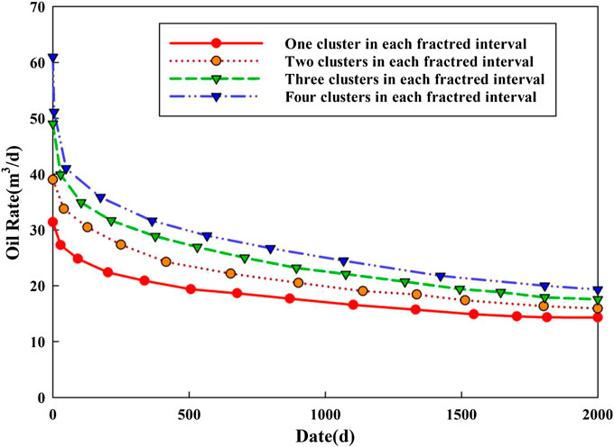
FIGURE 13. Daily oil production curve of different number of fracture clusters.

FIGURE 14

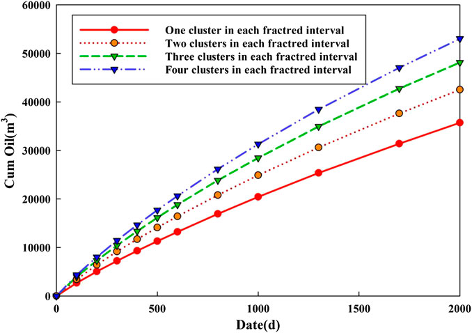
FIGURE 14. Cumulative oil production curve of different number of fracture clusters.

Fracture Flow Capacity

Fracture flow capacity is another important parameter to control horizontal well production. The variation of the oil rate under different fracture flow capacities is simulated by single factor analysis.

As can be seen from Figures 15, 16, the fracture flow capacity has a great impact on the early production stage of the horizontal well and a small impact on the later stage. In the early stage of horizontal well production, the wellbore of the horizontal well is mainly supplied from the volume fracturing region, which results in a high fracture flow capacity and fast fluid flow in the effective modification area. In the later stage, oil is supplied from the reservoir matrix region, which is not modified, has low permeability and relatively weak oil supply capacity, resulting in little difference in daily production in the later stage. However, although the fracture flow capacity increased in a linear manner, the growth rate in cumulative production decreased.

FIGURE 15

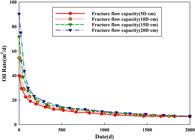
FIGURE 15. Daily oil Production Curve of Different Fracture Flow Capacity.

FIGURE 16

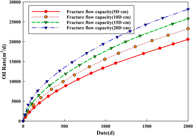
FIGURE 16. Cumulative oil production curve of different fracture flow capacity.

Conclusion

According to the seepage characteristics, the mathematical model of multiple media seepage in volume fracturing horizontal wells is established. The model takes into account the dual media composed of the fracture grid and the matrix formed by the coupling of artificial fracture and natural fracture, and a seepage model for the matrix region considering the trigger pressure gradient is established. In addition, the fluid-solid coupling effect in the tight reservoir is considered in the model, and the basic mathematical model of the stress field is established based on the principle of effective stress and the constitutive relation of rock skeleton. In addition, the mathematical model of stress field-seepage field for volume fracturing horizontal wells in tight reservoir is formed by combining with the seepage model. Finally, based on the rock mechanics characteristics of glutenite and taking into account the impact of Young's modulus, Poisson's ratio, initial permeability value and other parameters, the permeability stress crossing dynamic model is improved, and the fluid-solid coupling productivity model for volume fracturing horizontal wells is formed.

TABLE 1

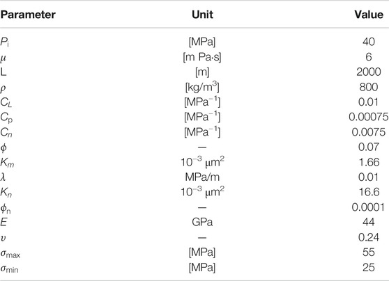
TABLE 1. Basic parameters of tight reservoir used in calculation.

Data Availability Statement

The raw data supporting the conclusions of this article will be made available by the authors, without undue reservation.

Author Contributions

All the authors have contributed to the conception and design of the productivity model. LT was mainly responsible for the construction of the capacity model, XC and PW were responsible for the solution and validation of the capacity model, and HW was responsible for the sensitivity analysis of the capacity model. The first draft was written by XC, and was revised and confirmed by all the authors.

Conflict of Interest

The authors declare that the research was conducted in the absence of any commercial or financial relationships that could be construed as a potential conflict of interest.

Acknowledgments

The authors would like to acknowledge the funding by the project (51974329) sponsored by the National Natural Science Foundation of China and the project (2016ZX05047–005–001) sponsored by the National Major Science and Technology Projects of China.

Glossary

$K_m$matrix permeability, 10⁻³ μm²
$v_m$fluid flow rate in matrix, 10⁻³$\text{m/s}$
μfluid viscosity, $\text{mPa}\cdot \text{s}$
$\nabla P_m$the pressure gradient of the pore system in bedrock, MPa/m
$\lambda$trigger pressure gradient, MPa/m
$\varphi$matrix porosity, %
${\varphi }_{\text{0}}$initial formation porosity, %
$C_L$fluid compressibility, MPa⁻¹
$C_{\text{p}}$pore compressibility, MPa⁻¹
$P_{\text{i}}$initial reservoir pressure, MPa
$\rho$fluid density, kg/m³${\rho }_0$initial fluid density, kg/m³
$Q_m$cross flow rate, kg/m³∙s
$\alpha =L_{\text{m}}^2/12$form factor
L_mmatrix rock size, m
$C_{\text{m}}$matrix composite compressibility, MPa⁻¹
$P_n$natural fracture system pressure, MPa
$P_m$matrix system pressure, MPa
$K_n$natural fracture permeability, 10⁻³ μm²
$C_n$natural fracture compressibility, MPa⁻¹
${\varphi }_{\text{n}}$natural fracture porosity
$K_f$artificial fracture permeability, 10⁻³ μm²
$C_{\text{f}}$artificial fracture compressibility, MPa⁻¹
${\varphi }_f$artificial fracture porosity
$p_w$bottom hole flowing pressure, MPa
$d{\sigma }_{ij}$effective stress increment
$D_{ijkl}$elastic-plastic coefficient matrix tensor
$d{\epsilon }_{kl}$strain increment
${\epsilon }_{\text{ij}}$strain tensor
μdisplacement component
$f_i$volume force on one side
$\sigma$normal stress
$\tau$shearing strength
${\tau }_{\text{xy}}$the component of stress in the y direction on the x plane
$\alpha$effective stress sensitivity coefficient, MPa⁻¹
$E$Young’s modulus, GPa
$\upsilon$Poisson’s ratio
${\alpha }_E$relationship between Young’s modulus and effective stress sensitivity coefficient
${\alpha }_{\upsilon }$relationship between Poisson’s ratio and effective stress sensitivity coefficient
${\alpha }_K$relationship between initial permeability value and effective stress sensitivity coefficient
$c_1$Young’s modulus influence coefficient
$c_2$Poisson’s ratio influence coefficient
$c_3$initial permeability value influence coefficient
${\epsilon }_{\text{v}}$volumetric strain
$N_{i,mn}$system element basis function matrix of ${\Omega }_{m,n}$
$\nabla N_{i,mn}^T,\nabla N_{i,mn}$transpose of matrix
$P_{i,m}$element node pressure matrix of ${\Omega }_m$
Vany function on the boundary
$\sigma$total stress of reservoir rock
${\sigma }^{\prime }$effective stress
MSystem mass matrix
$F_{\Gamma }$load vector
CSystem damping matrix
Lhorizontal well length, m
${\sigma }_{\max }$maximum principal stress, MPa
${\sigma }_{\min }$minor principal stress, MPa

References

Brohi, I. G., Pooladi-Darvish, M., and Aguilera, R. (2011). Modeling fractured horizontal wells as dual porosity composite reservoirs-application to tight gas, Shale gas and tight oil cases. Fairbanks, AK: Society of Petroleum Engineers.

Google Scholar

Brown, M., Ozkan, E., Raghavan, R., and Kazemi, H. (2011). Practical solutions for pressure-transient responses of fractured horizontal wells in unconventional shale reservoirs. SPE Reservoir Eval. Eng. 14 (06), 663–676. doi:10.2118/125043-pa

CrossRef Full Text | Google Scholar

Cao, J., James, L. A., and Johansen, T. E. (2015). A new coupled axial-radial productivity model for horizontal wells with application to high order numerical modeling. Abu Dhabi, UAE: Society of Petroleum Engineers.

Google Scholar

Doe, T., Lacazette, A., Dershowitz, W., and Knitter, C. (2013). “Evaluating the effect of natural fractures on production from hydraulically fractured wells using discrete fracture network models.” in Unconventional Resources Technology Conference, Denver, CO, August 12–14, 2013. doi:10.1190/urtec2013-172

CrossRef Full Text | Google Scholar

Friehauf, K. E., Suri, A., and Sharma, M. M. (2009). A simple and accurate model for well productivity for hydraulically fractured wells. SPE Prod. Oper. 25 (04), 453–460. doi:10.2118/119264-pa

CrossRef Full Text | Google Scholar

Hu, J., Zhang, C., Rui, Z., Yu, Y., and Chen, Z. (2017). Fractured horizontal well productivity prediction in tight oil reservoirs. J. Petrol. Sci. Eng. 151, 159–168. doi:10.1016/j.petrol.2016.12.037

CrossRef Full Text | Google Scholar

Jackson, M. D., Gomes, J. L. M. A., Mostaghimi, P., Percival, J. R., Tollit, B. S., Pavlidis, D., et al. (2013). Reservoir modeling for flow simulation using surfaces, adaptive unstructured meshes, and control-volume-finite-element methods. Austin, TX: Society of Petroleum Engineers. doi:10.2118/163633-MS

CrossRef Full Text | Google Scholar

Jianjun, L., Xiangui, L., Yareng, H., and Shengzong, Z. (2002). Study on fluid-solid coupling seepage in low permeability reservoir. J. Rock Mech. 21 (1):88–92 [in Chinese].

Google Scholar

Johansen, T. E., James, L., and Cao, J. (2015). Analytical coupled axial and radial productivity model for steady-state flow in horizontal wells. IJPE 1 (4), 290–307. doi:10.1504/ijpe.2015.073538

CrossRef Full Text | Google Scholar

Li, K., and Li, L. (2012). A new production model by considering the pressure sensitivity of permeability in oil reservoirs. Abu Dhabi, UAE: Publisher Society of Petroleum Engineers.

Google Scholar

Liu, R., Jiang, Y., Huang, N., and Sugimoto, S. (2018). Hydraulic properties of 3D crossed rock fractures by considering anisotropic aperture distributions. Adv. Geo-Energy Res. 2 (2), 113–121. doi:10.26804/ager.2018.02.01

CrossRef Full Text | Google Scholar

Ran, Q., and Li, S. (1997). Study on dynamic model of physical property parameters in numerical simulation of fluid-solid coupled oil reservoirs. Petrol. Explor. Dev. 024 (003), 61–65 [in Chinese].

Google Scholar

Ren, L., Su, Y. L., Zhan, S. Y., and Meng, F. K. (2019). Progress of the research on productivity prediction methods for stimulated reservoir volume (SRV)-fractured horizontal wells in unconventional hydrocarbon reservoirs. Arab. J. Geosci. 12 (6), 184. doi:10.1007/s12517-019-4376-2

CrossRef Full Text | Google Scholar

Sennhauser, E. S., Wang, S., and Liu, M. X. (2011). A practical numerical model to optimize the productivity of multistage fractured horizontal wells in the cardium tight oil resource. Alberta, Canada: Society of Petroleum Engineers.

Google Scholar

Stalgorova, E., and Mattar, L. (2012). Analytical model for history matching and forecasting production in multifrac composite systems. Alberta, Canada: Society of Petroleum Engineers.

Google Scholar

Yang, X., Guo, B., and Zhang, X. (2019). Use of a new well productivity model and post-frac rate-transient data analysis to evaluate production potential of refracturing horizontal wells in shale oil reservoirs. Charleston, VA: Society of Petroleum Engineers.

Google Scholar

Yin, D., Liu, K., and Sun, Y. (2019). A new model for pressure sensitive effect calculation considering rock characteristic parameters of tight reservoirs. Spe. Reservoirs. 26 (05), 71–75, 117 [in Chinese].

Google Scholar

Yuliang, S., Wendong, W., and Guanglong, S. (2014). Composite flow model for horizontal Wells with SRV fracturing. J. Pet. Sci. 35 (3) [in Chinese].

CrossRef Full Text | Google Scholar

Zhang, K., Jia, N., Li, S., and Liu, L. (2019a). Static and dynamic behavior of CO2 enhanced oil recovery in shale reservoirs: experimental nanofluidics and theoretical models with dual-scale nanopores. Appl. Energy. 255, 113752. doi:10.1016/j.apenergy.2019.113752

CrossRef Full Text | Google Scholar

Zhang, K., Jia, N., Li, S., and Liu, L. (2018). Thermodynamic phase behaviour and miscibility of confined fluids in nanopores. Chem. Eng. J. 351, 1115–1128. doi:10.1016/j.cej.2018.06.088

CrossRef Full Text | Google Scholar

Zhang, K., Jia, N., and Liu, L. (2019b). CO2 storage in fractured nanopores underground: phase behaviour study. Appl. Energy. 238, 911–928. doi:10.1016/j.apenergy.2019.01.088

CrossRef Full Text | Google Scholar

Zhang, K., Jia, N., and Liu, L. (2019c). Generalized critical shifts of confined fluids in nanopores with adsorptions. Chem. Eng. J. 372, 809–814. doi:10.1016/j.cej.2019.04.198

CrossRef Full Text | Google Scholar

Zhang, K., Liu, L., and Huang, G. (2020). Nanoconfined water effect on CO 2 utilization and geological storage. Geophys. Res. Lett. 47 (15). doi:10.1029/2020GL087999

CrossRef Full Text | Google Scholar

Zhang, N., and Abushaikha, A. S. (2019). Fully implicit reservoir simulation using mimetic finite difference method in fractured carbonate reservoirs. Abu Dhabi, UAE: Society of Petroleum Engineers.

Google Scholar

Zhao, K., and Du, P. (2019). Performance of horizontal wells in composite tight gas reservoirs considering stress sensitivity. Adv. Geo-Energ. Res. 3 (3), 287–303. doi:10.26804/ager.2019.03.07

CrossRef Full Text | Google Scholar