Synchronizing Stability Analysis and Region of Attraction Estimation of Grid-Feeding VSCs Using Sum-of-Squares Programming

Grid-synchronizing Stability (GSS) is an emerging issue related to grid-feeding voltage-source converters (VSCs). Its occurrence is primarily related to the non-linear dynamics of a type of vastly applied synchronization unit – Phase-locked Loops (PLL). Dynamic characterization and modeling for the GSS analysis can be achieved using a simplified system model, which is a second-order and autonomous non-linear equation, but with the presence of an indefinite damping term. As revealed and demonstrated in this work, this indefinite damping effect can result in an inaccurate Region-of-Attraction (ROA) estimation of the traditional Equal Area Principle (EAP)-based method. To overcome this issue and achieve a valid ROA estimation, this paper adopts the sum-of-squares (SOS) programming technique, which is a numeric optimization method with SOS relaxations. The development and implementation of the SOS program for ROA estimation are presented. Numerical case studies and time-domain verifications demonstrate that this method is valid for GSS analysis, and an almost precise estimation is achieved in the first quadrant. This evidence makes the SOS method a promising tool for GSS analysis because the GSS problem is most concerned with the stability within the first swing cycle, i.e., in the first quadrant.

Introduction

Voltage-source converters (VSCs) are becoming ubiquitous in electric power systems. According to their functionalities, they can be broadly classified as either grid-feeding and grid-forming. Grid-feeding VSCs are widely employed in bulk power systems for the grid integration of renewable power generations (RPGs) (Teodorescu et al., 2011) and for the interconnection of AC systems through high-voltage-dc (HVDC) transmission techniques (Flourentzou et al., 2009), etc. The primary control objective of a grid-feeding VSC is to process the electric power of different forms into a form that is acceptable to the grid. To achieve this with a high quality, the frequency and phase information of the grid voltage to which the VSC is connected should be detected. This is typically fulfilled with a type of vastly applied synchronization unit−the Phase-locked Loop (PLL). With the help of the PLL, the active and reactive power outputting from the VSCs is decoupled and can be controlled independently; moreover, the frequency of the VSC tends to closely follow the frequency of the grid. Although this fast phase-tracking and frequency-following feature of the PLL is beneficial for the performance of the VSC power controls, it can result in an adverse effect on the transient frequency stability of the power system (Gonzalez-Longatt, 2016). Countermeasures can be taken in this regard; for instance, by augmenting ancillary controls on VSCs (Gonzalez-Longatt, 2016; Sanchez et al., 2019) so that they can contribute to the frequency response of the system. Aside from this issue, the PLL also poses adverse effects on the small-signal stability of the VSC itself if not properly designed (Zhang et al., 2017a). This issue frequently occurs and is of particular interest under a weak AC grid condition, when its stability impact can be systematically assessed through impedance-based methods (Harnefors et al., 2007; Cespedes and Sun, 2014; Rygg et al., 2016; Zhang et al., 2018; Wang and Blaabjerg, 2019).

The above-exposed adverse impacts of the PLL greatly motivate the advancement and development of non-PLL-based synchronization schemes and associated VSC controls. Among these, the Virtual Synchronous Generator (VSG) control (Zhong and Weiss, 2011; D'Arco et al., 2015) and the Virtual Oscillator Control (VOC) (Johnson et al., 2014, 2016; Sinha et al., 2017) are very popular. Specifically, the VSG controls eliminate the use of PLL by mimicking the behavior of a Synchronous Generator (SG), whereas the VOC achieves non-PLL synchronization by utilizing the intrinsic features of particular types of non-linear oscillators, e.g., Van der Pol oscillator. With the VSG control, the typical droop controller (Ashabani, 2014) as employed by the SG can be readily implemented in VSCs. The VOC, on the other hand, exhibits some intrinsic droop-like behavior according to Sinha et al. (2017). These features bring a universal synchronization scheme and power-sharing ability to VSCs, which enables them to form and compose an electric system with the absence of SGs, thus giving them the name “grid-forming” VSCs. This trait has facilitated the fast emergence and development of VSC-based systems, e.g., smart grids (Ashabani, 2014).

Although VSG controls and VOCs are successful in small-scale and autonomous electric systems, like smart grids, their applicability in bulk power systems is still under discussion. One of the difficulties lies in the fundamental and scientific problem of how thousands of self-organized oscillators behave when they are coupled in circuits and what consequences this will bring (Stankovski et al., 2019). This is an open question in the field of coupled oscillators and, although it is not the topic of this paper, the behavioral characterization and understanding of the diverse non-linear oscillators existing in various types of VSCs seems to be crucial to answering this question. To this end, this paper will dig into a non-linear stability phenomenon associated with the PLL that is emerging in grid-feeding VSCs, i.e., grid-synchronizing stability (GSS) (Zhang et al., 2017b, 2020; Geng et al., 2018; Han et al., 2018; Hu et al., 2019; Taul et al., 2019; Wu and Wang, 2020; He et al., 2020). Please note that for brevity, the term “grid-feeding” will be omitted in later analysis.

To understand the GSS issue, a concise system model, preferably possessing a certain level of physical implication, needs to be developed. To this end, authors in Zhang et al. (2017b, 2020), Hu et al. (2019), and Taul et al. (2019) have developed a simplified model of the grid-VSC system for the GSS analysis, which is essentially a second-order and autonomous non-linear equation, referred to as the GSS model in later analysis. More appealingly, this GSS model is similar to the classic swing equation of the SG, due to which the GSS mechanism can be qualitatively elucidated according to the theory of SG. For example, the Equal Area Principle (EAP) developed for the SG can be used for this purpose (Zhang et al., 2017b, 2020; Hu et al., 2019). The obtained mechanism of GSS inspires many studies on stability-oriented control and parameter designs, e.g., the coordinated control schemes for the Low Voltage Ride Through (LVRT) (Geng et al., 2018; Han et al., 2018; He et al., 2020) and the PLL parameter design (Wu and Wang, 2020). The EAP can also help in achieving a quantitative evaluation of the Critical Clearing Time (CCT) of the GSS. However, the accuracy of the predicted CCTs, as shown in Zhang et al. (2020), is dependent on a properly chosen parameter k (a parameter used in Zhang et al. (2020) to estimate the area under the PLL-frequency and along the time axis). The occurrence of this parameter dependence lies in the fact that a successful application of the EAP requires the system to be dissipative. Unfortunately, the GSS model is not a dissipative system because of the indefinite damping term. Therefore, it can be maintained that the parameter k used in Zhang et al. (2020) is essentially a sort of compensation for this indefinite damping effect. However, this is not a formal way to resolve this issue, for which a valid method for GSS analysis which determines its stability region, i.e., its region-of-attraction (ROA) estimation, needs to be developed.

To achieve the estimation of ROA, the search and construction of a Lyapunov function (LF) would be the first step. Unfortunately, there are no generic and systematic methods for constructing LFs. However, an exception is that, provided the system is linear and stable or the linearized system is a Hurwitz system, there exists a quadratic-type LF that can be constructed through several systematic methods (Khalil, 2002). However, this condition (i.e., the system is Hurwitz) is quite strict in practice, which limits its applications, e.g., the linearized system of the GSS model is indeed not a Hurwitz system. Aside from this general difficulty in finding the LF, the search for the LF applied to the GSS analysis is even more difficult because of the indefinite damping effect, which is not a trivial problem in theory either (Freitas and Zuazua, 1996). It can be seen that the analytic construction of the LF is rather difficult, particularly for the GSS analysis; therefore, this paper will turn to the numeric methods (Genesio et al., 1985; Prajna et al., 2002), where the Sum-of-Squares (SOS) programming technique (Prajna et al., 2002) will be adopted due to its capability in both LF construction and ROA estimation through numeric optimization. Further, these functionalities can be flexibly programmed and implemented in SOSTOOLs, which is a toolbox for MATLAB (Prajna et al., 2002).

Through the SOS programming technique, the primary objective of this paper is to achieve an improved ROA estimation for the GSS analysis along with a detailed elucidation of its algorithmic implementation. Accuracy of the obtained ROA estimation with the GSS model is verified by time-domain simulations in PSCAD/EMTDC, where a switching VSC model with detailed control systems is employed. To the authors' best knowledge, this is the first attempt to apply SOS programming techniques to solve the GSS problem of grid-feeding VSCs. In addition, the obtained results and algorithmic implementation can be useful references for other advanced applications, e.g., multi-converters analysis in smart grids.

GSS Problem and the Indefinite Damping Effect

This section aims at demonstrating the previously mentioned indefinite damping effect and its impacts on the accuracy of EAP-based ROA estimation. To this end, the GSS problem, along with its analysis models, will be first introduced, although in a concise manner as this has been well-examined in existing works (e.g., Zhang et al., 2017b, 2020; Geng et al., 2018; Hu et al., 2019; Taul et al., 2019). The study system adopted is shown in Figure 1; it is composed of a three-phase VSC and a Thevenin equivalent grid. The VSC control system consists of a current vector control loop and a PLL. Since most of the grid-feeding VSCs are of high power and connected to a relatively high-voltage power grid, the line impedances are assumed to be purely inductive. This simplification also results in a concise GSS model, as will be shown next.

FIGURE 1

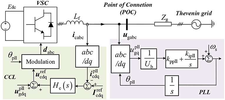
Figure 1. Single line diagram of a typical grid-VSC system.

The Original GSS Model and Its Variants

The Original GSS Model

According to Zhang et al. (2017b, 2020), Geng et al. (2018), Hu et al. (2019), and Taul et al. (2019), a simplified closed-loop model of the grid-VSC system for the GSS analysis can be formulated as Equation (1), which is the original GSS model. Basically, this model is obtained by assuming that the VSC current dynamics are quasi-steady in the timescale of the PLL dynamics (i.e., $I_{\mathrm{\text{cdq}}}^{\mathrm{\text{ref}}}\approx i_{\mathrm{\text{cdq}}}^{\mathrm{\text{pll}}}$) (Zhang et al., 2020). This quasi-steady current response can be approximately assured by adopting a relatively large current control bandwidth and compensating the grid-voltage disturbance through the feedforward control. Based on this, the original GSS model is obtained as

$\begin{array}{ll}\{\begin{array}{l}{\stackrel{\bullet }{x}}_{\text{pll}}=a_1{x}_{\text{pll}}-a_2(sin{\delta }_{\text{pll}}-sin{\delta }_0)\\ {\stackrel{\bullet }{\delta }}_{\text{pll}}=a_0{x}_{\text{pll}}-a_3(sin{\delta }_{\text{pll}}-sin{\delta }_0)\end{array}& (1)\end{array}$

The circuit representation of this GSS model is given in Figure 2A. By comparing it with the detailed system in Figure 1 it can be seen that the VSC current dynamics are simplified as a current source in the reference frame provided by the PLL (i.e., $I_{\mathrm{\text{cdq}}}^{\mathrm{\text{ref}}}\approx i_{\mathrm{\text{cdq}}}^{\mathrm{\text{pll}}}$). The PLL dynamics, on the other hand, are fully considered and modeled. Parameters in Equation (1) are related to the control and circuit parameters of the grid-VSC system, which are listed below

$\begin{array}{l}{a}_0=\frac{1}{1-k_{\text{ppll}}^{}{\bar{I}}_{\text{cd}}^{\text{ref}}{\bar{L}}_{\text{g}}/{\omega }_{\text{b}}},k_{\text{ipll}}^{}\frac{{\bar{I}}_{\text{cd}}^{\text{ref}}{\bar{L}}_s}{{\omega }_{\text{b}}}{a}_0=a_1^{},k_{\text{ipll}}{\bar{U}}_{\text{s}}{a}_0=a_2,\\ k_{\text{ppll}}^{}{\bar{U}}_{\text{s}}{a}_0=a_3,{\delta }_0={sin}^{-1}\left({\bar{I}}_{\text{cd}}^{\text{ref}}{\bar{L}}_{\text{g}}{\bar{\omega }}_{\text{s}}/{\bar{U}}_{\text{s}}\right)& (2)\end{array}$

In, ${\bar{I}}_{\mathrm{\text{cd}}}^{\mathrm{\text{ref}}}$,Ū_s are the per-unit VSC d-axis current and Thevenin grid voltage; ${\bar{\omega }}_{\mathrm{\text{s}}}$ is the per-unit synchronous angular frequency; ω_b = 2π · 50rad/s, ${\bar{\omega }}_{\mathrm{\text{s}}}=1$; under a normal condition Ū_s = 1, and Ū_s can be manipulated to emulate the grid voltage sags, which is used in later analysis. x_pll and δ_pll are the states of the PLL, where δ_pll = θ_pll − θ_s and ${\theta }_{\mathrm{\text{s}}}=\underset{}{\overset{}{\int }}{\omega }_{s}dt$. Moreover, it can be proven that a₀ > 0 holds true for a wide range of PLL parameters; please refer to the Appendices for the justification.

FIGURE 2

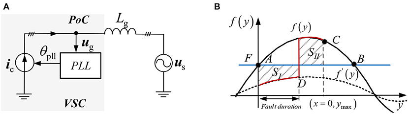
Figure 2. (A) Simplified circuit model for GSS analysis. (B) Mechanism illustration of the GSS.

The First Variant of the GSS Model

Stability analysis of non-linear systems is usually performed at the origin, i.e., $\stackrel{\bullet }{x}=f(x)$ with the condition f(0) = 0. This can be achieved by variable substitutions; for example, the equilibrium point(0, δ₀) of the original GSS model can be shifted to the origin by using the following substitutions: x = x_pll, y = δ_pll − δ₀, for which the resulting model is

$\begin{array}{ll}\{\begin{array}{l}\stackrel{\bullet }{x}=a_{1}x-a_2(sin(y+{\delta }_0)-sin({\delta }_0))\\ \stackrel{\bullet }{y}=a_{0}x-a_3(sin(y+{\delta }_0)-sin({\delta }_0))\end{array}& (3)\end{array}$

which is the first variant of the GSS model that will be used in the SOS-based ROA estimation later. Also, it can be readily checked that f(0) = 0 holds true for this model.

The Second Variant of the GSS Model

Although the first variant of the GSS model is sufficient for stability analysis, it gives little insight into the system's behavior. Therefore, a more instructive model for the mechanism analysis can be derived by a simple reformulation, i.e., by substituting x = a₀x − a₃(sin(y + δ₀) − sin(δ₀)) into Equation (3), the resulting equation is

$\begin{array}{ll}\{\begin{array}{l}\stackrel{\bullet }{x}=-{\displaystyle \underset{d(y)}{{\displaystyle \underbrace{(a_{3}cos(y+{\delta }_0)-a_1)}}}}{x}_{}+{\displaystyle \underset{F}{{\displaystyle \underbrace{b_{0}sin{\delta }_0}}}}-{\displaystyle \underset{f(y)}{{\displaystyle \underbrace{b_{0}sin(y+{\delta }_0)}}}}\\ \stackrel{\bullet }{y}=x\end{array}& (4)\end{array}$

which is the second variant of the GSS model that will be adopted for GSS mechanism analysis. In Equation (4), b₀ = a₀a₂−a₁a₃ and it can be obtained that b₀ is proportional to the magnitude of the grid-voltage Ū_s if it is written explicitly with the parameters in Equation (2), whereas F = b₀ sin y₀ is a constant value.

Next, based on the second variation of the GSS model, the GSS mechanism will be explained first by ignoring the damping term d(y), e.g., how the loss of synchronization of VSC occurs; then, the effect of the damping term d(y) on the accuracy of EAP in GSS analysis will be further discussed.

Mechanism Analysis of the GSS

First, by neglecting the damping term d(y) in Equation (4), the following model is obtained

$\begin{array}{ll}\{\begin{array}{l}\stackrel{\bullet }{x}=F-f(y)\\ \stackrel{\bullet }{y}=x\end{array}& (5)\end{array}$

from which it can be seen that it resembles the classic swing equation of the SG with zero dampings. Therefore, the well-known EAP (Kundur et al., 2004) developed for the SG can be used to elucidate the GSS mechanism of the VSC. This is illustrated as follows. First, characteristics of F and f(y) can be drawn in Figure 2B, where the stable equilibrium point A is obtained according to the condition F = f(y). If the VSC is subjected to a large grid voltage sag, this will lead to a drop of f(y) i.e., f′ < f, whereas F remains constant as explained earlier. Due to the occurrence of the mismatch between f′(y) and F, the following dynamic transition will take place:

(1) Initially, since f′ < F, both x and y start increasing along the characteristic of f′(y). If the grid fault is cleared at point D, the characteristics of f(y) will be changed back to their pre-fault state, i.e., f′ → f;

(2) Then, since f > F, x will decrease whereas y keeps increasing until x = 0, e.g., point C. The value of this condition (x = 0, y_max) can be obtained from the EAP where S_I = S_II is satisfied.

(3) Afterward, the state (x, y) will roll back along the characteristic of f(y) and finally settle down at the original steady-state point (i.e., point A). This is because the system is usually assumed to be dissipative in EAP-based analysis.

In Figure 2B, the trace from (1) to (2) is highlighted with the red line, which is known as the first swing cycle in the context of an SG for transient stability analysis (Kundur et al., 2004). Based on this process, it can be readily obtained that if the EAP is not satisfied when the state reaches the critical point B (i.e., S_I ≠ S_II, at B), then the VSC will be exposed to the danger of first swing cycle instability, i.e., the loss of synchronization.

Indefinite Damping Effect on the Accuracy of EAP in GSS Analysis

The above analysis explains the GSS mechanism with the help of EAP. Although the obtained result gives insight into the GSS problem, it may not be accurate due to the neglect of the system damping, more importantly, the ignored damping may not be positive as assumed. In fact, the damping term d(y) observed in the GSS model is indefinite in terms of its sign. This contradicts the assumption of the EAP-based analysis and can give rise to inaccurate results. The following example will demonstrate how this indefinite damping affects the accuracy of the EAP-based ROA estimation of GSS.

If the EAP is used for the ROA estimation, its LF can be formulated as:

$\begin{array}{ll}V(x,y)=\frac{1}{2}{x}^2-{\displaystyle {\int }_0^y}{b}_{0}sin{\delta }_0-b_{0}sin(\xi +{\delta }_0)d\xi & (6)\end{array}$

which mimics the summation of the kinetic and potential energy of an SG. Also, the level of V is set to the value at V_max(0, π − 2δ₀), which is known as the maximum potential energy in the system.

Based on Equation (6), the ROA estimation can be obtained and its contour is plotted in Figure 3. Theoretically, this ROA indicates that any trajectories starting within the ROA will be contained within the ROA and finally converge to the origin if the origin is asymptotically stable. To check the accuracy of the EAP-based ROA estimation, two types of trajectories with different initial states are given in the same figure, which are obtained from the dynamic system Equation (4). First, according to trajectory-I in Figure 3, it can be obtained that the estimated ROA is conservative because the initial state of this stable trajectory is not inside its estimation. However, this conservativeness is not consistent throughout the ROA, as indicated by trajectory-II, where the initial state of trajectory-II is inside the ROA but the result turns out to be unstable.

FIGURE 3

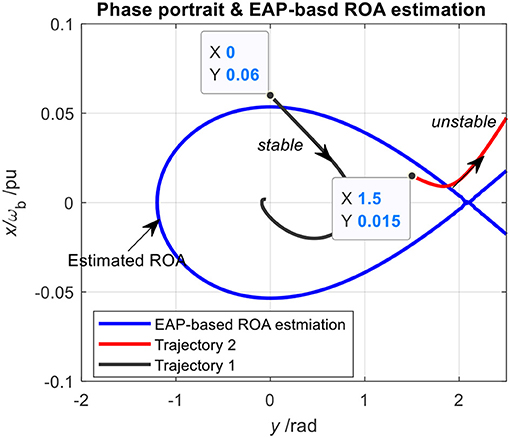
Figure 3. A case where EAP results in an inaccurate ROA ($I_{\mathrm{\text{cd}}}^{\mathrm{\text{ref}}}=1,k_{\mathrm{\text{scr}}}=2,{\alpha }_{\mathrm{\text{pll}}}=10$).

This analysis demonstrates that the EAP can result in misleading results if applied to the ROA estimation of the GSS, and the reason lies in the indefinite damping effect of the GSS model. Therefore, to overcome this issue and achieve an improved ROA estimation, the SOS programming technique (Prajna et al., 2002) will be adopted and presented in the next section. Other applications of this method, e.g., in the power system analysis, are conducted in Papachristodoulou and Prajna (2002), Anghel et al. (2013), and Shinsaku et al. (2018).

SOS Programming Technique-Based ROA Estimation of the GSS and Its Implementation in Sostools

This section will present how the SOS programming technique can be utilized for the LF construction and ROA estimation of the GSS analysis. The developed SOS program will be implemented in SOSTOOLs (Prajna et al., 2002), which is a toolbox for MATLAB and works as the interface and interpreter for translating formulated SOS problems into semidefinite programs (SDP), where the latter can be solved by various SDP solvers (Lieven and Boyd, 1996). To better illustrate this method applied to the GSS analysis, Lyapunov stability and its SOS program will be introduced first in a generic sense.

Lyapunov Stability and Its SOS Program

Global Stability and Its SOS Program

Considering an autonomous non-linear system ẋ = f(x), the Lyapunov stability theory states that if there exists an open set D ⊆ ℝ containing the origin (x = 0) and a continuously differentiable function V, such that V(0) = 0 and

$\begin{array}{ll}\{\begin{array}{l}V(x)>0,x\in D,x\ne 0\\ -\stackrel{\bullet }{V}(x)=-{\left(\frac{\partial V}{\partial x}\right)}^{T}f(x)\ge 0,x\in D\end{array}& (7)\end{array}$

then the origin is stable. If $-\stackrel{\bullet }{V}(x)>0$ for all x ∈ D,x ≠ 0, then the origin is asymptotically stable. If the limit ||x|| → ∞ so that V(x) → ∞ exists, then the origin is asymptotically stable.

In order to find a V satisfying Equation (7) by means of the SOSTOOLs, the non-negativity of those conditions can be relaxed to a problem of finding the SOS polynomials. For example, the first condition of Equation (7) can be relaxed to a problem of finding an SOS polynomial which satisfies: V(x) − l₁(x) ∈ SOS, where l₁(x) is a non-negative polynomial used to replace the non-polynomial constraint of x ≠ 0. This relaxation V(x) − l₁(x) ∈ SOS can be declared and solved by the SOSTOOLs with the in-built commands sosineq() and sossolve(), respectively. Here, the second command will call the SDP solvers for solutions. There are various SDP solvers available; this paper uses the STPT3 solver. Another frequently used command for declaring SOS polynomials is sossosvar().

This analysis illustrates that the non-negativity conditions of a semi-algebraic set can be relaxed to an SOS problem that is programmable and solvable. In fact, such relaxations can be formally fulfilled by the Positivstellensatz (P-satz) empty-set and its formulation; please refer to Tan and Packard (2004) for details. With the P-satz formulation, a generic procedure for formulating the SOS problem is shown below:

Step 1: Reformulate the original-set into the P-satz empty-set,

Step 2: Implement the formulated empty-set in SOSTOOLs and solve for solutions.

For example Equation (7) can be reformulated as the P-satz empty-set as (the asymptotic stability case):

$\begin{array}{ll}\begin{array}{l}\{x\in D|V(x)\le 0,l_1(x)\ne 0\}=\varphi \\ \{x\in D|-\stackrel{\bullet }{V}(x)\le 0,l_2(x)\ne 0\}=\varphi \end{array}& (8)\end{array}$

where l_1,2(x) are SOS polynomials used to replace the non-polynomial constraints x ≠ 0. Then, according to the P-satz theorem, this empty-set can be formulated as:

There exists s_0,1,2(x), such that

$\begin{array}{ll}\begin{array}{l}{s}_0-V(x)+l_1(x)=0\\ s_1+s_2{\left(\frac{\partial V}{\partial x}\right)}^{T}f(x)+l_2(x)=0\end{array}& (9)\end{array}$

where s_0,1,2(x) are SOS polynomials. Based on Equation (9), corresponding SOS problem can be immediately obtained as follows:

Find V(x) over s₂ such that

$\begin{array}{ll}\begin{array}{l}V(x)-l_1(x)\in SOS\\ -s_2{\left(\frac{\partial V}{\partial x}\right)}^{T}f(x)-l_2(x)\in SOS\end{array}& (10)\end{array}$

where Equation (10) can be declared and solved by SOSTOOLs with the above-mentioned commands, e.g., sosineq() and sossolve(). However, this SOS problem is bilinear in decision variables. To overcome this issue, s₂ and V(x) can be solved iteratively; this will be explained in more detail later.

Local Stability and Its SOS Program

The above global stability case demonstrates how an LF can be found using the SOS programming method. However, global stability is rare for non-linear systems; indeed, most of them exhibit local stability behavior around the origin. In this regard, the stability region, i.e., the determination of how far away the initial state can be from the origin while remaining stable, is of great usefulness for study. This can be achieved by finding the largest level for the LF while assuring the $-\stackrel{\bullet }{V}(x)\ge 0$, i.e., the ROA estimation. To achieve this estimation through SOS programming, the general idea is to first define an estimated ROA; then, define a subset contained in the estimated ROA; afterward, by enlarging this subset, the estimated ROA will be forced to expand due to the set containment; this process will finally result in an optimized estimation of the real ROA of the system.

Using the semi-algebraic sets to represent the above-given procedure, the following description is obtained: define a region Ω_c = {x ∈ ℝ|V(x) ≤ c} as an estimation of ROA and define a subset H_β: = {x ∈ ℝ|h(x) ≤ β} that is contained in Ω_c, i.e., H_β ⊆ Ω_c and h(x) is a given positive definite function. Therefore, Ω_c is forced to expand by enlarging H_β. Based on these sets, the SOS program for ROA estimation in a general sense can be developed according to the following steps.

Maximize β such that

$\begin{array}{ll}\begin{array}{l}\{x\in ℝ|h(x)\le \beta \}\subseteq \{x\in ℝ|V(x)\le c\}\\ \{x\in ℝ|V(x)\le c,x\ne 0\}\subseteq \{x\in ℝ|-\stackrel{\bullet }{V}(x)>0\}\end{array}& (11)\end{array}$

where the P-satz empty-set can be further obtained as:

$\begin{array}{ll}\begin{array}{l}\left\{x\in ℝ|h(x)\le \beta ,V(x)>c,V(x)\ne c\right\}=\varphi \\ \left\{x\in ℝ|V(x)\le c,\stackrel{\bullet }{V}(x)\ge 0,x\ne 0\right\}=\varphi \end{array}& (12)\end{array}$

Based on the procedure illustrated in Global Stability and Its SOS Program, and adding the non-negative condition of the LF, the following SOS problem for ROA estimation in a general sense can be finally obtained:

Maximize β over s₁, s₂, c such that

$\begin{array}{ll}\begin{array}{l}V-l_1\in SOS\\ -(\beta -h)s_1-(V-c)\in SOS\\ -\left({\left(\frac{\partial V}{\partial x}\right)}^{T}f+s_2(c-V)+l_2\right)\in SOS\end{array}& (13)\end{array}$

where l_1,2(x), s_1,2,3(x) are SOS polynomials. Since both V and c are decision variables, c only has a scaling effect on V; therefore c = 1 can be assumed during the implementation. Also, it is noted that this SOS problem is bilinear in decision variables (e.g., due to the multiplication terms: βs₁ and Vs₂). The issue can be addressed by using iterations and will be explained later. Besides, maximizing β can be fulfilled by using the bisection method or the in-built command sossetobj() in SOSTOOLs. Aside from this, there are other optimization methods available and one may refer to Nguyen et al. (2018) for extended reading.

SOS Program for the ROA Estimation of GSS

The above SOS programs for LF construction and ROA estimation are introduced in a general sense. When applied to the GSS analysis, some modifications to the program and procedure are required, which will be discussed in this section.

Recast the GSS Model

The first modification required is related to model compatibility. The SOS program requires the models or systems under study to consist of polynomial vector fields, i.e., f should be a vector of polynomials; however, the developed GSS models consist of non-polynomial vector fields. To make the model compatible with the SOS program, the GSS model can be recast through variable substitutions (Papachristodoulou and Prajna, 2002; Anghel et al., 2013; Shinsaku et al., 2018), e.g., by using the following substitutions:

$\begin{array}{ll}\begin{array}{l}{x}_1=sin(y+{\delta }_0)-sin({\delta }_0)\\ x_2=cos(y+{\delta }_0)-cos({\delta }_0)\\ x_3=x\end{array}& (14)\end{array}$

the GSS model (Equation 3) (i.e., the first variant) can be recast into

$\begin{array}{ll}\begin{array}{l}{\stackrel{\bullet }{x}}_1=(x_2+cos{\delta }_0)·(a_0{x}_3-a_3{x}_1)\\ {\stackrel{\bullet }{x}}_2=-(x_1+sin{\delta }_0)·(a_0{x}_3-a_3{x}_1)\\ {\stackrel{\bullet }{x}}_3=a_1{x}_3-a_2{x}_1\end{array}& (15)\end{array}$

where an additional constraint on x₁ and x₂ is that

$\begin{array}{ll}g={(x_1+sin{\delta }_0)}^2+{(x_2+cos{\delta }_0)}^2-1=0& (16)\end{array}$

It is noticed that this additional algebraic constraint assures that the recast system has the same dimension as the GSS model. More importantly, the recast system (Equation 15) consists of polynomial vector fields.

SOS Program for ROA Estimation

The recast GSS model uses polynomial vector fields so that the SOS-based ROA estimation as introduced in Local Stability and Its SOS Program can be applied. However, another modification on the empty-set (Equation 12) should be made due to the additional constraint g = 0 in the recast system. The result is shown below

$\begin{array}{ll}\begin{array}{l}\{x\in ℝ|h(x)\le \beta ,V(x)>1,V(x)\ne 1,g=0\}=\varphi \\ \{x\in ℝ|V(x)\le 1,\stackrel{\bullet }{V}(x)\ge 0,x\ne 0,g=0\}=\varphi \end{array}& (17)\end{array}$

Then, based on this empty-set, its SOS program can be formulated as:

Maximize β over s₁, s₂, t₁, t₂ such that

$\begin{array}{ll}\begin{array}{l}V-l_1\in SOS\\ -((\beta -h)s_1+(V-1)+t_1·g)\in SOS\\ -\left({\left(\frac{\partial V}{\partial x}\right)}^{T}f+s_2(1-V)+l_2+t_2·g\right)\in SOS\end{array}& (18)\end{array}$

where l_1,2(x) and s_1,2(x) are given SOS polynomials which can be declared with the command sossosvar() in SOSTOOLS. The additional functions t_1,2(x) are polynomials and must not necessarily be SOS, and they can be declared in SOSTOOLs by using another command, sospolyvar().

Implementation of the SOS Program in SOSTOOLs

As mentioned above, due to the occurrence of bilinear decision variables, the SOS program in Equation (18) cannot be solved directly through the SOSTOOLs. This issue can be resolved through an iteration process as follows. By dividing the decision variables into two groups, two sub-processes are obtained for solving variables of these two groups iteratively, and for each sub-process, the SOS problem is linear in decision variables and can be solved by the SOSTOOLs. In this paper, decision variables β and V are defined as the first group, whereas variables s₁, s₂, t₁, t₂, t₃ are defined as the second group.

To start the first sub-process, solving for s₁, s₂, t₁, t₂, β and V should be initialized. Initialization of β is straightforward: it can be set as a small value, whereas the initialization of V is equivalent to the problem of finding an initial LF satisfying Equation (17). This new problem can be readily tackled if the linearized system is a Hurwitz system. However, this condition does not apply for the GSS analysis where the linearized system of Equation (15) is typically not a Hurwitz system. Therefore, the initial LF will be found through the SOS method as well, where a modified program based on Equation (18) is used and shown below:

Find V₀ over s₂, t₁, t₃ such that

$\begin{array}{ll}\begin{array}{l}{V}^{(0)}-l_1\in SOS\\ -\left({\left(\frac{\partial V^{(0)}}{\partial x}\right)}^{T}f+s_2({\beta }^{(0)}-h)+l_2+t_2·g\right)\in SOS\end{array}& (19)\end{array}$

This program is obtained according to the sets containment of Equation (17), from which an initial V⁽⁰⁾ can be found. With the obtained initial values of V⁽⁰⁾ and β⁽⁰⁾, variables $s_1^{(0)},s_2^{(0)},t_1^{(0)},t_2^{(0)}$ can be solved from the last two equations in Equation (18); this is the first sub-process. Then, the second sub-process proceeds with the obtained $s_1^{(0)},s_2^{(0)},t_1^{(0)},t_2^{(0)}$, and by solving Equation (18), V⁽¹⁾ and β⁽¹⁾ are updated, which are the inputs for the next iteration. This iterative procedure will repeat until the change of β^(k) is no longer evident, i.e., ceases if the condition |β^(k+1) − β^(k)| ≤ ε is true. Based on this illustration, the complete SOS algorithm for the ROA estimation of GSS is given in Figure 4.

FIGURE 4

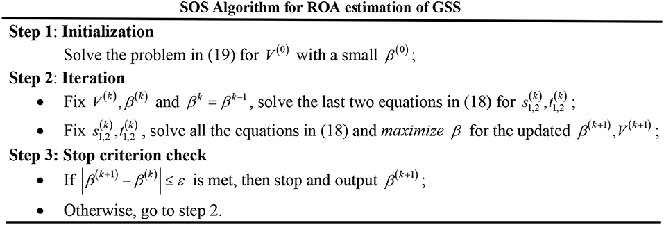
Figure 4. SOS algorithm for ROA estimation of GSS.

In the algorithm, the following commands are used: (1) declaration of functions: sospolyvar(), sossosvar(); (2) declaration of SOS equalities and inequalities soseq(), sosineq(); (3) solve problems: sossolve(),sossetobj(); (4) return of solutions: sosgetsol(). Other functions and configurations used are: $l_{1,2}(x)={10}^{-6}{\displaystyle \sum _{k=1}^3}{x}_k^2$, $h(x)={\displaystyle \sum _{k=1}^3}{x}_k^2$, the tolerance ε = 10⁻⁴; s₁(x), s₂(x) are declared as SOS polynomials and the order of them is 2; t₁(x), t₂(x) are declared as polynomials with an order of 1. V is declared as a polynomial function [with the condition V(0) = 0] and the order is 2.

Numeric Case Studies and Time-Domain Verifications

This section will present numeric case studies of the SOS-based ROA estimation of GSS. For comparison, the results of EAP-based ROA estimation [i.e., based on Equation (6)] and the exact ROA [i.e., obtained from the numeric simulation of Equation (3)] are shown as well. Finally, to verify the validity and accuracy of the estimated ROA, time-domain simulations in PSCAD/EMTDC are conducted where a switching VSC is used and the overall system configuration is the same as in Figure 1.

Numeric Case Studies of ROA Estimation

Under a Weak AC Grid Condition

In the first place, ROA estimation under a weak grid (i.e., the short circuit ration is k_scr = 2) is analyzed. After running the developed SOS program for ROA estimation with 23 iterations, it returns an LF of the recast system (Equation 15) as

$\begin{array}{ll}\{\begin{array}{l}V(x)=0.312x_1^2+0.0358x_1·x_2-0.025x_1·x_3-0.333x_2^2\\ -0.015x_2^{}{x}_3^{}-0.002x_3^2\\ \beta =2.998\end{array}& (20)\end{array}$

where some items with extremely small coefficients are ignored. Then, by substituting Equation (14) into Equation (20), the LF for the GSS model is obtained:

$\begin{array}{ll}\begin{array}{l}{V}_{\text{GSS}}=0.025x\left(\sin \left(y+{\delta }_0\right)-0.5\right)+0.333(\cos \left(y+{\delta }_0\right)\hfill \\ {-0.866)}^2+0.312{\left(\sin \left(y+{\delta }_0\right)-0.5\right)}^2+0.036(\cos \hfill \\ \left(y+{\delta }_0\right)-0.866)\left(\sin \left(y+{\delta }_0\right)-0.5\right)\hfill \\ +0.002x^2-0.015x\left(\cos \left(y+{\delta }_0\right)-0.866\right)\hfill \end{array}& (21)\end{array}$

By setting the level of V_GSS as V_GSS = 1, the contour indicates the optimized ROA estimation of the GSS under this strong grid condition. Next, a comparative study of ROA estimations from the SOS, the EAP, and the numeric simulation is conducted and the results are shown in Figure 5.

FIGURE 5

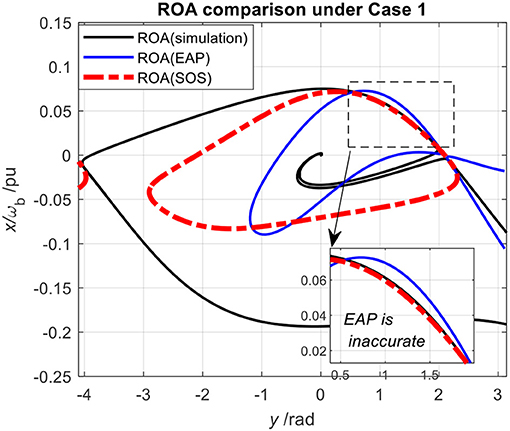
Figure 5. ROA comparisons under a weak grid condition (α_pll = 10, $I_{\mathrm{\text{cd}}}^{\mathrm{\text{ref}}}=1$, k_scr = 2).

According to Figure 5, first, it can be seen that the ROA estimation from EAP is inaccurate since part of its boundary is outside the exact ROA. This inaccuracy of EAP in GSS analysis has already been pointed out in Figure 3, which is due to the indefinite damping effect. By contrast, the SOS-based method successfully resolves this issue since its contour is completely contained in the exact ROA. Although the result is still conservative, the estimation is indeed greatly improved with the SOS optimization if compared to the result of the EAP. Moreover, since the GSS analysis is most concerned with the stability of the first swing cycle, from this perspective, the SOS-based ROA estimation is rather satisfactory since its estimation is similar to the exact ROA in the first quadrant.

Besides, one may notice that the shape of ROA with EAP is different from that in Figure 3. This is because in Figure 3 the estimated ROA is based on the second variant of the GSS model, i.e., Equation (4), whereas this analysis is based on the first variant of the GSS model, i.e., Equation (3).

Under a Relatively Strong AC Grid Condition

Next, the ROA estimation under a relatively strong grid will be analyzed, where the short circuit ration of k_scr = 5 is used. Similarly, the SOS is run in SOSTOOLs, and after 37 iterations, it returns an LF of the recast system (Equation 15) as

$\begin{array}{ll}\{\begin{array}{l}V(x)=0.108x_1^2+0.065x_1^{}{x}_2^{}-0.007x_1^{}{x}_3^{}+0.261x_2^2\\ -0.006x_2^{}{x}_3^{}+0.001x_3^2\\ \beta =3.8389\end{array}& (22)\end{array}$

where the items with extremely small coefficients are ignored. Then, substituting Equation (14) into Equation (20) yields the LF for the GSS model, which is:

$\begin{array}{ll}\begin{array}{l}{V}_{\text{GSS}}=-0.007x-0.523cos(y+0.2)-0.107sin(y+0.2)\\ +0.083cos(2y+0.0003)-0.006xcos(y+0.2)\\ -0.007xsin(y+0.2)+0.001x^2+0.452\end{array}& (23)\end{array}$

where V_GSS = 1 indicates the optimized ROA estimation under this strong grid condition.

Then, a similar comparative analysis to the first case study is conducted and the results are presented in Figure 6. According to this figure, again, it is immediately concluded that the EAP-based ROA estimation is inaccurate since part of its boundary is outside the exact ROA. The SOS-based method, on the contrary, is well-contained in the exact ROA, indicating a correct but conservative ROA estimation. Moreover, it can be seen that in terms of the GSS analysis, where the focus is on the stability of the first swing cycle, the SOS-based method is rather accurate since its ROA estimation is similar to the exact one if compared in the first quadrant.

FIGURE 6

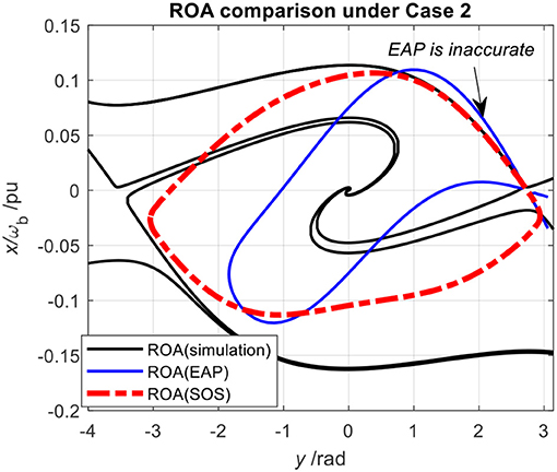
Figure 6. ROA comparisons under a strong grid (α_pll = 10, $I_{\mathrm{\text{cd}}}^{\mathrm{\text{ref}}}=1$, k_scr = 5).

On the other hand, interestingly, when comparing the result of the ROA estimation under the strong grid (i.e., Figure 6) to that under the weak grid (i.e., Figure 5), it can be seen that the conservativeness of the ROA estimation tends to improve when the grid becomes strong.

Time-Domain Simulation and Verification

To verify the numeric results, particularly the validity and accuracy of the SOS-based ROA estimation, time-domain simulations are conducted in the PSCAD/EMTDC. To provoke the GSS issue, the VSC in simulation is perturbed by a large grid voltage dip. In detail, the magnitude of the Thevenin grid voltage is dropped down to 0.2 p.u. at 1 s. In addition, two types of fault clearing time (FCT) are considered: the shorter one is 135 ms and the longer one is 140 ms. Corresponding time instants at which the fault is cleared are marked by points A and B in the following figures.

First, in Figure 7A, time-domain waveforms of states relevant to the GSS model under two types of FCTs are presented. It can be seen that under a longer FCT, i.e., 140 ms, the states are unstable after the fault is cleared, whereas under a shorter FCT, i.e., 135 ms, the system is stable after the fault is cleared. This simulation implies that the state trajectory of the GSS model at point B (i.e., under FCT = 140 ms) is anticipated to be outside the ROA, whereas the one at point A (i.e., under FCT = 135 ms) should be inside the ROA.

FIGURE 7

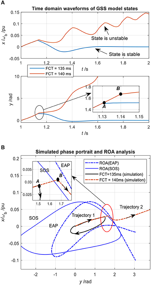
Figure 7. (A) Time-domain waveforms of states relevant to GSS model. (B) State trajectories in comparison with ROA estimations.

In order to check if the same conclusion can be drawn from the estimated ROA, the same state trajectories under two types of FCTs are plotted together with the ROA estimations from the SOS and EAP, which are shown in Figure 7B. From this figure, it can be seen that point B is indeed located outside the ROA of the SOS method, while point A is inside its ROA estimation. This analysis demonstrates that: (1) the SOS-based ROA estimation is correct and quite accurate since the difference between the longer and shorter FCT is very small; (2) the simplified model for the GSS analysis is feasible and valid, otherwise the estimated ROA would be inaccurate.

On the other hand, this time-domain study again demonstrates that the EAP-based ROA estimation is inaccurate and leads to a misleading stability result, as can be seen from Figure 7B, where point B is inside the estimated ROA while the time-domain result turns out to be unstable.

Conclusions

This paper discussed the GSS issue and its ROA estimation of grid-feeding VSCs. First, the indefinite damping effect in GSS analysis is revealed and its impact on the accuracy of the EAP-based ROA estimation is discussed. Then, the SOS programming technique is employed to address this indefinite damping issue and to achieve an improved ROA estimation, in which the SOS program for ROA estimation of GSS is developed and its implementation in SOSTOOLs is elaborated. Finally, comparative numeric studies of the ROA estimations with different methods are performed. The obtained numeric results are verified by time-domain simulations in PSCAD/EMTDC.

Based on the presented analyses, it can be concluded that the SOS-based method can successfully overcome the indefinite damping issue encountered by the EAP-based method. Although the estimated ROA is still conservative, it is nonetheless improved through SOS optimization. Particularly, the estimated ROA is similar to the exact ROA in this first quadrant. This evidence demonstrates that this method is even more useful for GSS analysis because the GSS problem is most concerned with the stability of the first swing cycle, i.e., the first quadrant of the estimated ROA.

Besides, the presented methodology and results can be useful references and can lay the foundation for other advanced applications in the future, e.g., smart grids with multi-converters.

Data Availability Statement

The datasets generated for this study are available on request to the corresponding author.

Author Contributions

CZ and MM contributed to the conception and design of the study. ZL and XC organized case studies. CZ wrote the first draft of the manuscript. All authors contributed to manuscript revision, read, and approved the submitted version.

Funding

This work was supported in part by NTNU (81617922) and in part by the National Natural Science Foundation of China (51837007).

Conflict of Interest

The authors declare that the research was conducted in the absence of any commercial or financial relationships that could be construed as a potential conflict of interest.

References

Anghel, M., Milano, F., and Papachristodoulou, A. (2013). Algorithmic construction of lyapunov functions for power system stability analysis. IEEE Trans. Circuits Syst. I Regular Pap. 60, 2533–2546. doi: 10.1109/TCSI.2013.2246233

CrossRef Full Text | Google Scholar

Ashabani, M. (2014). “Synchronous converter and synchronous-VSC- state of art of universal control strategies for smart grid integration,” in 2014 Smart Grid Conference (SGC) (Tehran), 1–8.

Google Scholar

Cespedes, M., and Sun, J. (2014). Impedance modeling and analysis of grid-connected voltage-source converters. IEEE Trans. Power Electron. 29, 1254–1261. doi: 10.1109/TPEL.2013.2262473

CrossRef Full Text | Google Scholar

D'Arco, S., Suul, J. A., and Fosso, O. B. (2015). A virtual synchronous machine implementation for distributed control of power converters in SmartGrids. Electr Power Syst Res. 122, 180–197. doi: 10.1016/j.epsr.2015.01.001

CrossRef Full Text | Google Scholar

Flourentzou, N., Agelidis, V. G., and Demetriades, G. D. (2009). VSC-based HVDC power transmission systems: an overview. IEEE Trans. Power Electron. 24, 592–602. doi: 10.1109/TPEL.2008.2008441

CrossRef Full Text | Google Scholar

Freitas, P., and Zuazua, E. (1996). Stability results for the wave equation with indefinite damping. J. Different. Equat. 132, 338–352.

Google Scholar

Genesio, R., Tartaglia, M., and Vicino, A. (1985). On the estimation of asymptotic stability regions: State of the art and new proposals. IEEE Trans. Autom. Control. 30, 747–755.

Google Scholar

Geng, H., Liu, L., and Li, R. (2018). Synchronization and reactive current support of PMSG based wind farm during severe grid. IEEE Trans. Sustain. Energy 9, 1596–1604. doi: 10.1109/TSTE.2018.2799197

CrossRef Full Text | Google Scholar

Gonzalez-Longatt, F. M. (2016). Impact of emulated inertia from wind power on under-frequency protection schemes of future power systems. J. Modern Power Syst. Clean Energy 4, 211–218. doi: 10.1007/s40565-015-0143-x

CrossRef Full Text | Google Scholar

Han, G., Zhang, C., and Cai, X. (2018). Mechanism of frequency instability of full-scale wind turbines caused by grid short circuit fault and its control method. Trans. China Electrotech. Soc. 33, 2167–2175. doi: 10.19595/j.cnki.1000-6753.tces.170085

CrossRef Full Text | Google Scholar

Harnefors, L., Bongiorno, M., and Lundberg, S. (2007). Input-admittance calculation and shaping for controlled voltage-source converters. IEEE Trans. Indus. Electron. 54, 3323–3334. doi: 10.1109/TIE.2007.904022

CrossRef Full Text | Google Scholar

He, X., Geng, H. J., Xi, and Guerrero, J. M. (2020). Resynchronization analysis and improvement of grid-connected VSCs during grid faults. IEEE J. Emerg. Select. Topics Power Electr. doi: 10.1109/JESTPE.2019.2954555. [Epub ahead of print].

CrossRef Full Text | Google Scholar

Hu, Q., Fu, L., Ma, F., and Ji, F. (2019). Large signal synchronizing instability of PLL-based VSC connected to weak AC grid. IEEE Trans. Power Syst. 34, 3220–3229. doi: 10.1109/TPWRS.2019.2892224

CrossRef Full Text | Google Scholar

Johnson, B. B., Dhople, S. V., Hamadeh, A. O., and Krein, P. T. (2014). Synchronization of parallel single-phase inverters with virtual oscillator control. IEEE Trans. Power Electron. 29, 6124–6138. doi: 10.1109/TPEL.2013.2296292

CrossRef Full Text | Google Scholar

Johnson, B. B., Sinha, M., Ainsworth, N. G., Dörfler, F., and Dhople, S. V. (2016). Synthesizing virtual oscillators to control islanded inverters. IEEE Trans. Power Electron. 31, 6002–6015. doi: 10.1109/TPEL.2015.2497217

CrossRef Full Text | Google Scholar

Khalil, H. (2002). Nonlinear Systems, 3rd Edn. Upper Saddle River, NJ: Prentice Hall.

Google Scholar

Kundur, P., Paserba, J., Ajjarapu, V., Andersson, G., Bose, A., Canizares, C., et al. (2004). Definition and classification of power system stability IEEE/CIGRE joint task force on stability terms and definitions. IEEE Trans. Power Syst. 19, 1387–1401. doi: 10.1109/TPWRS.2004.825981

CrossRef Full Text | Google Scholar

Lieven, V., and Boyd, S. (1996). Semidefinite programming. SIAM Rev. 38, 49–95.

Google Scholar

Nguyen, T. T., Vu Quynh, N., Duong, M. Q., and Van Dai, L. (2018). Modified differential evolution algorithm: a novel approach to optimize the operation of hydrothermal power systems while considering the different constraints and valve point loading effects. Energies 11:540. doi: 10.3390/en11030540

CrossRef Full Text | Google Scholar

Papachristodoulou, A., and Prajna, S. (2002). “On the construction of Lyapunov functions using the sum of squares decomposition,” in Proceedings of the 41st IEEE Conference on Decision and Control (Las Vegas, NV), 3482–3487.

Google Scholar

Prajna, S., Papachristodoulou, A., and Parrilo, P. A. (2002). “Introducing SOSTOOLS: a general purpose sum of squares programming solver,” in Proceedings of the 41st IEEE Conference on Decision and Control (Las Vegas, NV), 741-746.

Google Scholar

Rygg, A., Molinas, M., Zhang, C., and Cai, X. (2016). A modified sequence-domain impedance definition and its equivalence to the dq-domain impedance definition for the stability analysis of ac power electronic systems. IEEE J. Emerg. Select. Topics Power Electron. 4, 1383–1396. doi: 10.1109/JESTPE.2016.2588733

CrossRef Full Text | Google Scholar

Sanchez, F., Cayenne, J., Gonzalez-Longatt, F., and Rueda, J. L. (2019). Controller to enable the enhanced frequency response services from a multi-electrical energy storage system. IET Generat. Transmission Distrib. 13, 258–265. doi: 10.1049/iet-gtd.2018.5931

CrossRef Full Text | Google Scholar

Shinsaku, I., Somekawa, H., Xin, X., and Yamasaki, T. (2018). Estimation of regions of attraction of power systems by using sum of squares programming. Electr. Eng. 100, 2205–2216. doi: 10.1007/s00202-018-0690-z

CrossRef Full Text | Google Scholar

Sinha, M., Dörfler, F., Johnson, B. B., and Dhople, S. V. (2017). Uncovering droop control laws embedded within the nonlinear dynamics of van der pol oscillators. IEEE Trans. Control Netw. Syst. 4, 347–358. doi: 10.1109/TCNS.2015.2503558

CrossRef Full Text | Google Scholar

Stankovski, T., Tiago, P., McClintock, P. V. E., and Stefanovska, A. (2019). Coupling functions: dynamical interaction mechanisms in the physical, biological and social sciences. Philos. Trans. R. Soc. A Math. Phys. Eng. Sci. 377. doi: 10.1098/rsta.2019.0039

PubMed Abstract | CrossRef Full Text | Google Scholar

Tan, W., and Packard, A. (2004). Searching for Control Lyapunov Functions Using Sums of Squares Programming. SIBI.

Google Scholar

Taul, M. G., Wang, X., Davari, P., and Blaabjerg, F. (2019). “An efficient reduced-order model for studying synchronization stability of grid-following converters during grid faults,” in 2019 20th Workshop on Control and Modeling for Power Electronics (COMPEL) (Toronto, ON), 1–7.

Google Scholar

Teodorescu, R., Liserre, M., and Rodriguez, P. (2011). Grid Converters for Photovoltaic and Wind Power Systems. Chichester: John Wiley and Sons.

Google Scholar

Wang, X., and Blaabjerg, F. (2019). Harmonic stability in power electronic-based power systems: concept, modeling, and analysis. IEEE Trans. Smart Grid 10, 2858–2870. doi: 10.1109/TSG.2018.2812712

CrossRef Full Text | Google Scholar

Wu, H., and Wang, X. (2020). Design-oriented transient stability analysis of PLL-synchronized voltage-source converters. IEEE Trans. Power Electron. 35, 3573–3589. doi: 10.1109/TPEL.2019.2937942

CrossRef Full Text | Google Scholar

Zhang, C., Cai, X., and Li, Z. (2017b). Transient stability analysis of wind turbines with full-scale voltage source converter. Proc. CSEE 37, 4018–4026. doi: 10.13334/j.0258-8013.pcsee.162359

CrossRef Full Text | Google Scholar

Zhang, C., Cai, X., Li, Z., Rygg, A., and Molinas, M. (2017a). Properties and physical interpretation of the dynamic interactions between voltage source converters and grid: electrical oscillation and its stability control. IET Power Electron. 10, 894–902. doi: 10.1049/iet-pel.2016.0475

CrossRef Full Text | Google Scholar

Zhang, C., Cai, X., Rygg, A., and Molinas, M. (2018). Sequence domain SISO equivalent models of a grid-tied voltage source converter system for small-signal stability analysis. IEEE Trans. Energy Conv. 33, 741–749. doi: 10.1109/TEC.2017.2766217

CrossRef Full Text | Google Scholar

Zhang, C., Cai, X., Rygg, A., and Molinas, M. (2020). Modeling and analysis of grid-synchronizing stability of a Type-IV wind turbine under grid faults. Int. J. Electr. Power Energy Syst. 117:105544. doi: 10.1016/j.ijepes.2019.105544

CrossRef Full Text | Google Scholar

Zhong, Q., and Weiss, G. (2011). Synchronverters: inverters that mimic synchronous generators. IEEE Trans. Indus. Electron. 58, 1259–1267. doi: 10.1109/TIE.2010.2048839

CrossRef Full Text | Google Scholar

Appendices

If the PLL bandwidth is defined as the decaying factor of its time-domain response (i.e., α_pll = εω_n, ε = 0.707),$k_{\mathrm{\text{ppll}}}^{}=2{\alpha }_{\mathrm{\text{pll}}},k_{\mathrm{\text{ipll}}}^{}=2{\alpha }_{\mathrm{\text{pll}}}^{\mathrm{\text{2}}}$ are obtained. Furthermore, if ${\alpha }_{\mathrm{\text{pll}}}<\frac{{\omega }_{\mathrm{\text{b}}}}{2{\bar{I}}_{\mathrm{\text{cd}}}^{\mathrm{\text{ref}}}{\bar{L}}_{\mathrm{\text{g}}}}=\frac{{\omega }_{\mathrm{\text{b}}}{k}_{\mathrm{\text{scr}}}}{2{\bar{I}}_{\mathrm{\text{cd}}}^{\mathrm{\text{ref}}}}$, it obtains a₀ > 0. k_scr is the short circuit ratio (SCR) of the grid. Usually, this inequality ${\alpha }_{\mathrm{\text{pll}}}<\frac{{\omega }_{\mathrm{\text{b}}}{k}_{\mathrm{\text{scr}}}}{2{\bar{I}}_{\mathrm{\text{cd}}}^{\mathrm{\text{ref}}}}$ is satisfied because the critical value of the right-hand side evaluated under an extreme case (e.g., k_scr = 2, ${\bar{I}}_{\mathrm{\text{cd}}}^{\mathrm{\text{ref}}}=1$) is sufficiently large for a commonly employed PLL, i.e., ${\alpha }_{\mathrm{\text{pll}}}^{}<{\alpha }_{\mathrm{\text{pll}}}^{\mathrm{\text{cr}}}={\omega }_{\mathrm{\text{b}}}^{}$ normally holds true. As a result, inequality a₀ > 0 holds true as well.