Improvement of Wind Power Assessment in Complex Terrain: The Case of COSMO-1 in the Swiss Alps

This work contains a series of calculations that explore the wind power potential in Switzerland using the Numerical Weather Prediction model COSMO-1. The model's performance was validated in complex terrain by comparing the modeled hourly wind speed to weather stations across Switzerland's mountains during a 2 year period. For wind-exposed stations, mean RMSE was found to be 2.87 m/s, mean MBE 0.03 m/s and mean correlation 0.51. For the wind-sheltered stations, model performance is slightly worse. We use the modeled wind speeds to calculate potential power production, and find capacity factors up to 0.42. With the modeled power time series, we show that in a hypothetical fully renewable Swiss power system, turbine siting can have a significant effect on imports, which may attain values from6 TWh/a to 13.3 TWh/a. Most importantly, the lowest import values are found for high wind power scenarios. When selecting locations with high capacity factors only (from random subsets of available locations), influence on import becomes small. An annual wind energy target of 6 TWh can be reached with as little as 1914 MW of turbine capacity, but this requires turbines to be built at relatively high elevations (mean turbine elevation 2967 above sea level). The lower the mean elevation of the wind turbines, the more capacity is required to reach the same production target. Furthermore, when restricting potential installations to locations deemed suited by the Swiss federal government (as laid out in the policy document “Konzept Windenergie Schweiz”), the capacity required to produce 6 TWh annually was found to be 2508 MW.

1. Introduction

Switzerland has recently adopted a law to decommission its nuclear power plants at the end of their lifetime, and to significantly boost the production from renewables. In order to achieve these goals, it has developed the Energy Strategy 2050 (Federal Department of the Environment Transport Energy and Communications DETEC, 2018). Large increases in power production from renewable sources such as wind and solar will have to be realized if they are to replace Switzerland's nuclear capacity, which currently produces 32,8% of Switzerland's annual (2016) electricity supply (Bundesamt für Energie, 2017). Previous work has shown that wind energy has a favorable seasonal profile to complement hydropower and photovoltaics (PV) (Dujardin et al., 2017; Kruyt et al., 2017), and as such is worth investigating further in view of the Energy Strategy 2050, which is the focus of this paper.

1.1. Wind Resource Assessment Using NWPs

Initial wind resource assessment is often based on numerical weather prediction (NWP) models. In relatively flat terrain, wind fields are rather uniform, which allows for relatively straightforward extrapolation of results. Similarly, NWP model resolution does not need to be very high for accurate assessment. In complex terrain such as the Alps however, the wind climate in the lower boundary layer is strongly influenced by the topography, which causes e.g., local speed up effects through gap flows and orography (Mayr et al., 2007; Lewis et al., 2008). Hence accurate modeling of the wind climate in complex terrain requires spatial resolutions that capture these topographic features.

At the same time, long simulations or measurements are required so that seasonal and inter-annual variability can be assessed. The computational demands resulting from these two requirements (high spatial resolution and long simulations) make it unrealistic to simulate large areas such as the entire Swiss alpine domain for wind potential assessment.

Various methods have been developed in attempts to overcome these shortcomings by reducing computational demands. Most notably, diagnostic methods forego the time derivatives of the partial differential equations describing conservation of mass and momentum that govern NWP models, the so-called Navier-Stokes equations. The thus assumed steady state flow can be solved at lower computational expense. However, dynamic processes such as flow splitting, vortex shedding and thermally induced circulations cannot be accurately represented in such schemes (Truhetz, 2010). Examples of such models include WindSim (WindSim, 2018) and 3DWind (Berge et al., 2006).

Other methods exist, that attempt to avoid the computational costs of solving the Navier Stokes equations at high resolution by using statistical relations instead. In such statistical models, (often linear) regression is used to interpolate relations between observations (synoptic scale wind fields, topography) and predictands: in this case near surface wind fields. As noted by Truhetz (2010) however, “Because of the terrain-induced decoupling effects between predictors and predictands these methods have conceptual shortcomings in the Alpine region.” (For a more detailed classification of wind resource modeling see Truhetz (2010) ).

1.2. Wind Resource Assessment in the Alps

Specifically for the alpine domain, a number of studies have attempted to assess the wind potential in sections of the Alps. Truhetz (2010) developed a hybrid method of using dynamic, diagnostic and statistical models to derive annual mean wind speeds and Weibull parameters for the Austrian Alps in a resolution of 100 x 100 m. This was then used to assess the wind potential in Austria (Truhetz et al., 2012; Winkelmeier et al., 2014). Draxl and Mayr (2011) found the best locations in the Austrian Alps to be mountain ridges (with median wind speeds of 7 m/s and potential of 1,600–2,900 kWh/a/m²). In Switzerland, a statistical method was used to interpolate measurements onto a grid with a horizontal resolution of 100 x 100 m (Bundesamt für Energie BFE et al., 2004). This method was expanded upon in the Alpine windharvest project (Schaffner and Remund, 2005). More recently, a Swiss Wind Atlas was developed using the diagnostic model WindSim in combination with measurement series, where the latter were used to scale the model output to obtain mean annual wind speeds (Koller and Humar, 2016). For the alpine domain, they report absolute differences (error) of 1.0 m/s (valley) to 1.5 m/s (mountains) in calculated mean annual wind speeds compared to long standing measurements. These mean annual wind speeds were combined with regional and national interests to produce a selection of areas that the federal government recommends suitable for wind power development. The document describing these areas is called the “Konzept Windenergie Schweiz” (roughly translated here as Swiss Wind energy concept) (Bundesamt für Energie BFE and Bundesamt Für Umwelt, 2004; Bundesamt für Raumentwicklung, 2017).

Other notable efforts to use statistical downscaling techniques specifically for Switzerland include the work of Helbig et al. (2017), who use sub-grid topography parametrization (the Laplacian of terrain elevations and mean square slope) to statistically downscale coarse-scale wind speeds from the ARPS model. Their results show large correlations with higher resolution wind speeds from the same model. Winstral et al. (2016) developed a statistical downscaling technique based on the exposure to / sheltering from wind based on high resolution (25 m) DEM data. They assess the performance of COSMO-2 (2.2 km resolution) and COSMO-7 ( 6.6 km resolution) forecasts and were able to reduce the biases in those forecasts with their downscaling technique.

Various efforts have also been undertaken to quantify the effect of increased horizontal resolution in NWPs on wind speed prediction. Jafari et al. (2012) compare model resolutions for several areas including a domain within Switzerland, and conclude that in complex terrain the increase in horizontal resolution from 9 to 3 km leads to significant improvements in weekly-averaged wind speed predictions. Dierer et al. (2009) compare COSMO-7 (6.6 km resolution) to COSMO-2 (2.2 km resolution) wind speed forecasts for 5 locations in Switzerland and conclude that for all sites, the increase in resolution from COSMO-7 to COSMO-2 improves results.

1.3. Outline and Goals

The aim of this paper is to investigate the role of wind energy in the dynamics of highly renewable Swiss electricity scenarios. Specifically, since previous work indicates that wind power at higher elevations may have benefits in terms of the seasonal production profile (Kruyt et al., 2017), special attention is paid to the alpine domain. To this end we choose, contrary to previously described assessment methods, to not simplify the physics by using steady-state simplifications or statistical predictions. Rather, we opt to use a fully non-hydrostatic NWP with relatively high spatial resolution. The COSMO-1 model, described in more detail in section 2 below, has been running for roughly 2 years at a hourly time step. While this is arguably a rather brief period for wind resource assessment, we want to focus on improving the wind assessment in Alpine terrain, which can be judged from the new dataset. For this terrain it is acknowledged that physical simplifications in the modeling approach have severe shortcomings. Therefore, the choice to compromise on the length of wind speed records rather than the physical representation of the phenomena is made.

This work aims to contribute to the understanding of wind power in complex terrain and thereby help the cost-efficient transition to a more sustainable electricity supply. Although the work is focussed on Switzerland, the methodology and results are applicable to any mountainous terrain. It is to our understanding the first time a mesoscale NWP model is coupled with model of the Swiss national power system to asses the influence of turbine siting on both required import and turbine capacity. To our knowledge, thus far all wind resource or potential assessments for Switzerland (Bundesamt für Energie BFE and Bundesamt Für Umwelt, 2004; Schaffner and Remund, 2005; Koller and Humar, 2016) have to some extent been based on statistical methods, thereby foregoing the physics governing the actual flows. It is about time to see how a fully physical model compares.

This paper is structured as follows: Firstly, the performance of the COSMO-1 model is assessed by comparing the modeled wind speeds to weather stations across Switzerland. Next, we calculate power time series from the modeled wind speeds and use these in an existing energy model to investigate different wind turbine siting scenarios in Switzerland, where the constraints defined in the aforementioned policy document “Swiss wind energy concept” are also investigated. Section 2, describes the models and calculations used throughout this work. Next, section 3 discusses the main results from the aforementioned calculations and finally we draw conclusions and provide an outlook in section 4.

2. Methods

2.1. COSMO-1

The Consortium for small-scale modeling (COSMO) maintains the COSMO family of NWP models. These non-hydrostatic, mesoscale NWP models are used by research institutes and meteorological services around the world (Consortium for Small-scale Modeling, 2017). In this work, we use the output of the COSMO-1 model, which has a horizontal resolution of 0.01°, which corresponds to 1.11 km N-S and 0.74–0.78 km E-S. Vertically, it features 80 levels with smooth level vertical (SLEVE) terrain following coordinates. The SLEVE scheme allows for smaller terrain features to decay faster than larger ones, thus reducing computational errors and allowing for a smooth transition to the upper homogeneous levels (Schär et al., 2002; Leuenberger et al., 2010). This version of the COSMO model has been operational at the Swiss national weather service since the end of 2015, providing us with a little more than 2 years of hourly (reanalysis) data. The 10 m wind speeds are used for verification against the measurement stations, while interpolating between the two nearest vertical levels gives the wind speed at 100 m above the surface for scenario analysis. With the exclusion of lakes, the number of 0.01° pixels within Switzerland amounts to 48657.

2.2. IMIS Network

The IMIS station network (Lehning et al., 1999; SLF, 2016), consisting of 198 stations around the Alps and Jura mountains, is operated by the Swiss institute for snow and avalanche research SLF. These stations are located in pairs with a wind station at a wind-exposed location and a snow station at a wind-sheltered location, which is generally also at slightly lower elevation. In addition, a small number of reference stations exist. All stations measure temperature, humidity and wind speed. Data are averaged over 30 min. The wind stations are located at elevations from 1936 (Amden - Mattstock) to 3345 (Zermatt - Platthorn) m.a.s.l. While the snow stations range from 1513 to 2914 m.a.s.l. In total there are 177 stations within Switzerland that have more than 1 year of data within the period that COSMO-1 has been operational. A map with the locations of the stations is shown in Figure 1. The other, well-known network of weather stations in Switzerland is the SwissMetNet. However the data from these stations are assimilated in the COSMO models and can therefore not be used for validation.

FIGURE 1

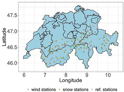
Figure 1. The IMIS stations.

2.3. Validation of COSMO-1

The performance of the COSMO-1 model in complex terrain is assessed by comparing the modeled wind speeds against the IMIS stations described above. Since IMIS stations record their data on 30 min intervals, their data is averaged over hourly intervals so it can be compared against COSMO-1's hourly output. We then assess correlation for pairwise-complete observations, as well as root mean square error (RMSE) and mean bias error (MBE).

2.4. Power Transformation

The wind speed time series of each COSMO-1 pixel are transformed to power output by applying a power curve. To this end we use the power curve of a wind turbine commonly found in Switzerland, the Enercon E82. Although site-specific wind turbine selection can arguably increase local wind power production, this is a rather complex matter and therefore refrained from. See Kruyt et al. (2017) for a discussion on wind turbine sensitivity for Switzerland, as well as a more detailed description of the methodology. We use the wind speeds at 100 meter above the surface for the analysis. Using the Enercon's power curve, we then calculate 1 MW power time series for each pixel. In subsequent modeling steps, we can then easily scale the production in each pixel to achieve various targets. Analogous to Kruyt et al. (2017) the power production is corrected to account for reduced air density at higher elevations.

2.5. Wind Energy Potential

It is worthwhile to distinguish between various types of wind energy potential. Loosely based on Hoogwijk and Graus (2008) and Hoogwijk et al. (2004), we can distinguish:

• The theoretical potential, which relates to the power that can be extracted from the wind (limited by Betz' law).

• The technical potential is the theoretical potential reduced by the conversion efficiencies of the turbines, losses due to maintenance etc

• The geographical potential is the technical potential reduced by land-use constraints. As this inherently also involves political choices, we have dubbed it geographical/political potential.

• The economical potential is that part of the above which is feasible at current competitive cost levels.

• The market potential is the amount of wind energy that can be integrated into the market given constraints on demand and supply patterns, institutional barriers and subsidies.

These various forms of energy potential have been schematically represented in Figure 2. The work in this paper is mainly concerned with the technical potential, although comparisons are made to the Swiss wind energy concept (Bundesamt für Energie BFE and Bundesamt Für Umwelt, 2004; Bundesamt für Raumentwicklung, 2017), which describes areas deemed suited for wind power development by the federal government, and as such touches onto the geographical potential.

FIGURE 2

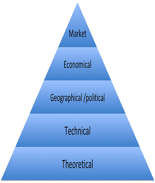
Figure 2. The various forms of wind energy potential, described in more detail in 2.5.

Seen from the perspective of a wind developer at a potentially profitable location, the modeling presented in this paper is only a first step in the wind resource assessment process. For the development of an actual wind farm, such modeling is usually followed by on-site measurements, modeling of turbulence intensities to select an appropriate turbine and micro-siting, and, in case of a multi-turbine wind farm, the modeling of wind turbine interactions such as wake effects (ADB, 2014; Sharma et al., 2018)

2.6. Modeling Switzerland's Power Supply

The Swiss power system is simulated to investigate the effect of different turbine locations on the dynamics of the power system. We deploy a model that is described in detail in Dujardin et al. (2017), with simulations run for the period of 01-01-2016 through 31-12-2017, two full years. This model uses the time series of Switzerland's electricity production and consumption to compute the amount of energy that can not be generated indigenously. In this work we simulate a fully renewable Swiss power supply, where all current nuclear capacity is replaced by renewables. This implies that 47% of the current demand¹ will be covered by new renewables (PV, wind, geothermal). In our model, 4.4 TWh/a will come from geothermal energy as a constant base load, and the remaining 49.38 TWh for the 2-year simulation period come from a combination of PV and wind energy. We investigate various wind targets of 8, 12, and 24 TWh for the 2 simulation years. In each of these cases, the remainder of this 49.38 TWh comes from PV. The PV time series are generated from satellite data while we model production from panels located in urban areas. Panels are located following population density, representing the idea that mainly rooftops will be used. The remaining 53% of the demand in our generation portfolio is met by the current Swiss hydropower installations. For the run-of-river plants, we directly use the production time series for the given period (33 TWh for the 2 years). For the storage hydropower plants, we use the time series of production and reservoir levels to compute the energy equivalent inflow into the system (33 TWh). We also use the plants' and reservoirs' characteristics to get a nationally aggregated capacity for storing and releasing the aforementioned energy inflow. The model's behavior can be summarized by these 3 steps: 1. From the national demand time series, compute the residual demand by subtracting the non-dispatchable sources (run-of-river, PV, wind, geothermal); 2. Compensate for the mismatch using short-term storage (pumped hydropower) within its capacity; 3. Use the flexibility of storage-hydropower to compensate for the remaining mismatch, within its capacity. Finally, the sum of what could not be alleviated by storage hydropower corresponds to the amount of energy that could not be transferred from the summer period to the winter period. This winter energy deficit is referred to as required import. For more detailed information about this power and energy balance model, we refer to Dujardin et al. (2017).

As mentioned, total production from PV and wind amounts to 49.38 TWh over the 2 years in order to reach bi-annual self sufficiency and a fully renewable power system. We investigate bi-annual wind power targets of 8, 12, and 24 TWh, where the remainder of the bi-annual 49.38 TWh ‘new-renewables' target is met by PV in all scenarios. While a potential of 4 TWh/a in 2050 is often mentioned (Hirschberg et al., 2005; Brugger et al., 2009; Abhari et al., 2012; Prognos, 2012; VSE, 2014; Bauer et al., 2017), this number appears to stem from reports dating back 14 years (Bundesamt für Energie BFE and Bundesamt Für Umwelt, 2004; Hirschberg et al., 2005). In the mean time, global wind power development has continuously surpassed expectations, driving down prices (Ayuso and Kjaer, 2016) and rotor diameters have increased. Furthermore, increases in model resolution have shown the potential in complex terrain and at elevation to be significant (Draxl and Mayr, 2011; Truhetz et al., 2012; Kruyt et al., 2017). Because of these reasons, we feel a higher production target is most likely attainable. Also, previous work (Dujardin et al., 2017; Kruyt et al., 2017) has shown that wind power can have a beneficial effect on system stability and required import. Moreover, comparing several targets allows us to show the dynamics of the system.

The results and targets will from here on be presented as annual results and targets, rather than bi-annual. Although strictly not the same, this is done to increase the readability of the text and allow for quicker, intuitive comparison to other studies and targets. The main differences are that we do not enforce the production of any wind power target in 1 year, but allow for compensation between the 2 years. Similarly, national demand and supply are required to be balanced on a bi-annual basis instead of on an annual one.

2.7. Required Number of Wind Turbines

An important question is how many turbines are required to achieve a certain amount of annual wind energy production, and how this depends on the siting of those turbines. Specifically, as previous work has indicated that high elevation wind power may offer higher yields (Kruyt et al., 2017), we want to investigate the effect that locating turbines at higher elevations has on production and thereby, the required amount of turbines. In order to investigate this, we deploy a methodology where the maximum elevation at which turbines can be placed is varied iteratively, and look at the resulting amount of turbines required to reach the annual production target (4, 6, or 12 TWh/a). One methodological challenge is the fact that there are more locations (pixels) below 4,000 m.a.s.l than there are below 2,000 m.a.s.l. In order to make a ‘fair' comparison between scenarios, we take random subsets of a fixed size from the all locations below each maximum elevation cap, so that each scenario is based on the same amount of initial candidates. As this random process introduces an element of chance, we repeat this random draw 10 times for each elevation cap, in order to increase the robustness of the results. The size of this random subset will obviously have an influence on the results. The smaller this subset, the fewer locations with high capacity factors will be included, and thus more pixels (and thus turbines) are needed to reach the national production target. For too large a subset, insufficient pixels will be available below a low elevation threshold. As there is no “right” amount, we use the arbitrary amount of roughly 22,000 (out of the total of 48,657). To represent the fact that turbines require space, the amount of turbines that can be placed in one (0.01°) pixel is limited to 6 MW, corresponding to 3 2 MW turbines (Denholm et al., 2009; Meyers and Meneveau, 2012).

The resulting algorithm can thus be summarized in the following steps: 1. A random subset of fixed size is drawn from all pixels below the maximum allowed elevation for that iteration; 2. Capacity (6 MW max per pixel) is assigned to the pixel with the highest capacity factor, then the second highest and so on, until the annual production target is met; 3. The resulting nationally aggregated wind power time series is then used to run the electricity model described in the previous paragraph to asses its effects on the Swiss power system. 4. The steps above are repeated 10 times, after which the process starts for the next elevation maximum.

Due to the seasonality of hydropower production and electricity demand, the mismatch between supply and demand is highest in winter (Dujardin et al., 2017). To see if it would be worthwhile to place wind turbines focussed specifically at alleviating this ‘winter gap', we conduct the same calculation but this time sorting the COSMO-1 grid cells based on the capacity factor in the winter months (November through April). Hence the locations with best winter production are picked first, and not necessarily the locations producing the most throughout the year. It goes without saying that this second method will require more capacity to meet a similar target, since the targets are (bi-)annual ones.

3. Results and Discussion

3.1. Validation of COSMO-1 Against IMIS Weather Stations

Figures 3–5 show the results of the model validation comparing the hourly wind speeds of the model with the IMIS stations. Overall, it can be seen that the COSMO-1 model performs significantly better for wind-exposed stations than it does for wind-sheltered stations: From Figure 3 we can see that the RMSE is lower for the wind-exposed stations and has a smaller spread. Similarly, the correlation is higher for the wind-exposed stations and has a smaller spread (Figure 5). Lastly the MBE is almost zero for the wind-exposed stations, whereas it is 1.78 m/s for the wind-sheltered stations (Figure 4). Winstral et al. (2016) find a positive bias for sheltered locations when compared to COSMO-2 forecasts, while they find a negative bias for wind-exposed stations. It should be noted that their definition of sheltered and exposed is different from ours, as we take the IMIS station types (i.e., “snow” or “wind” stations, see Section 2), and Winstral et al. (2016) use the topographic position index (TPI), a measure of the staion's location relative to the mean elevation in a 2 km radius surrounding the station.

FIGURE 3

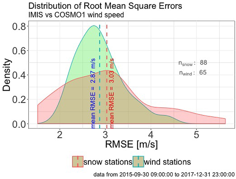
Figure 3. Root Mean Square Error (RMSE) between IMIS and COSMO-1 wind speeds. The plot shows the distribution of the individual RMSE's, that were calculated as the RMSE between each station's observed (measured) time series and the time series of the corresponding COSMO-1 grid cell.

FIGURE 4

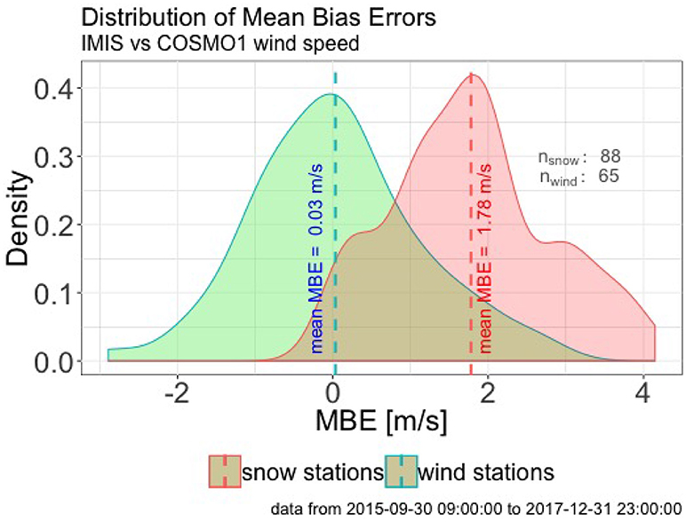
Figure 4. Mean Bias Error (MBE) between IMIS and COSMO-1 wind speeds. The plot shows the distribution of the individual MBE's, that were calculated as the MBE between each station's observed (measured) time series and the time series of the corresponding COSMO-1 grid cell.

FIGURE 5

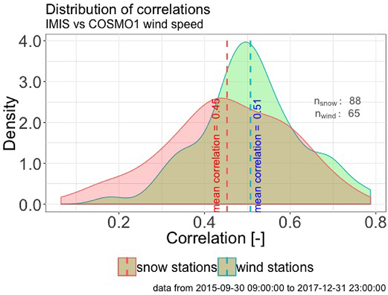
Figure 5. Correlations between IMIS and COSMO-1 wind speeds, for both wind- and snow stations. Correlation coefficients were calculated between the wind speed timeseries of each station and the wind speed timeseries of the corresponding COSMO-1 grid cell.

Table 1 summarizes these same data. We could not discern a significant relation between any of the error measures (MBE, RMSE) and the station's elevation. RMSE increased slightly with elevation for both wind (R² = 0.01) and snow stations (R² = 0.17), as did MBE ($R_{wind}^2=$ 0.07, $R_{snow}^2=$ 0.11) but these R² values prevent any strong conclusions. Similarly, correlation decreased slightly with elevation for the wind-sheltered stations (R² = 0.02), and no relation was found for the wind-exposed stations.

TABLE 1

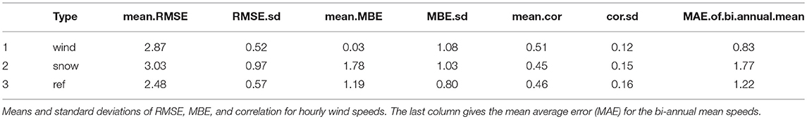
Table 1. COSMO-1 validation against IMIS stations, for wind-exposed “wind” stations, wind-sheltered “snow” stations and reference stations.

3.2. Comparison With Wind Atlas

In the analysis for the official Swiss wind atlas (windatlas.ch), Koller and Humar (2016) reported an absolute error of 1.0 m/s for valleys and 1.5 m/s for mountains in mean annual wind speeds. Comparing the bi-annual means of the COSMO-1 wind speed to the station data, we find a mean average error of 0.83 m/s for the wind-exposed stations. As these are the type of locations that are interesting from a perspective of wind power development, as opposed to the wind-sheltered stations, this is a significant improvement when compared to the Swiss wind atlas. Although it is unclear if the absolute error reported in Koller and Humar (2016) is based on one or all seven of their validation points², the fact that our calculations are based on 65 wind-exposed stations makes them significantly more robust.

3.3. Capacity Factor

We calculated capacity factors for each COSMO-1 pixel, defined as the actual production vs. the theoretical (i.e., rated) production. We account for forced outage and maintenance by assuming an availability factor of 96% (Williams, 2014). Although arguably in alpine environments there are additional factors to consider such as icing (Grünewald et al., 2012), at the same time losses due to icing reported from a Swiss test site are minimal (Barber et al., 2011) and with current blade heating technologies may be reduced to near zero³. Although one could incorporate a correction factor into the capacity factor calculation that accounts for additional downtime at higher elevations, the lack of reliable spatially distributed data would make this a rather arbitrary undertaking, and introduce more uncertainty than it resolves.

The calculated capacity factors are shown in Figure 6 and range from 0.01 to 0.42. If the capacity factor is calculated over just the winter months (November–April), the range increases from 0.01 up to 0.49.

FIGURE 6

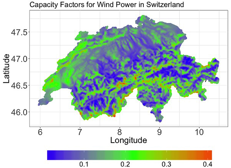
Figure 6. Capacity Factors, defined as the ratio of produced power vs rated power, with a correction for down time due to maintenance or other purposes.

3.4. Potential Import Reduction due to Turbine Siting

To assess the influence of wind siting scenarios on the resulting import for a renewable Swiss power supply, we run a set of simulations where we produce the entire wind power target from the time series of one COSMO-1 pixel. This is obviously an unrealistic scenario, however it does provide us with a range of influence on the power system. In other words, what is the influence wind power can have on overall system performance?

For annual wind targets of 4, 6, and 12 TWh/a, the unit power time series from each pixel is scaled to reach the desired target. The electricity model is then run to provide the required import, which we can display in the same pixel, thus creating a map that tells us how much import is needed should the entire wind target be produced from locations with such characteristics. This theoretical scenario provides some valuable insights. Producing 4 TWh/a of wind power from the characteristic wind time series from a single location can lead to a (bi-)annually self sufficient system with as little as 9 TWh/a of imports, whereas the ‘worst' locations can lead to an increase of 26.2% (11.4 TWh/a). For higher annual wind power targets of 6 or 12 TWh/a the range of required import to balance the system increases. Imports to balance a power system producing 6 Twh/a range from 8.1 to 11.7 TWh/a, and a power system with 12 TWh/a of wind power requires at least 6 TWh/a and at most 13.3 TWh/a. The resulting maps are shown on the left hand side of Figure 7. What these results tell us is 2-fold: one, there is great disparity in the wind potential across Switzerland, and two; As the amount of wind power in the system increases (from 4 TWh/a to 12 TWh/a), the range of required imports increases. This means that accurate wind turbine siting becomes more important as the installed capacity is increased. But also, as the share of wind power in the electricity mix increases, it becomes possible to make the system (bi-)annually self-sufficient with less imports.

FIGURE 7

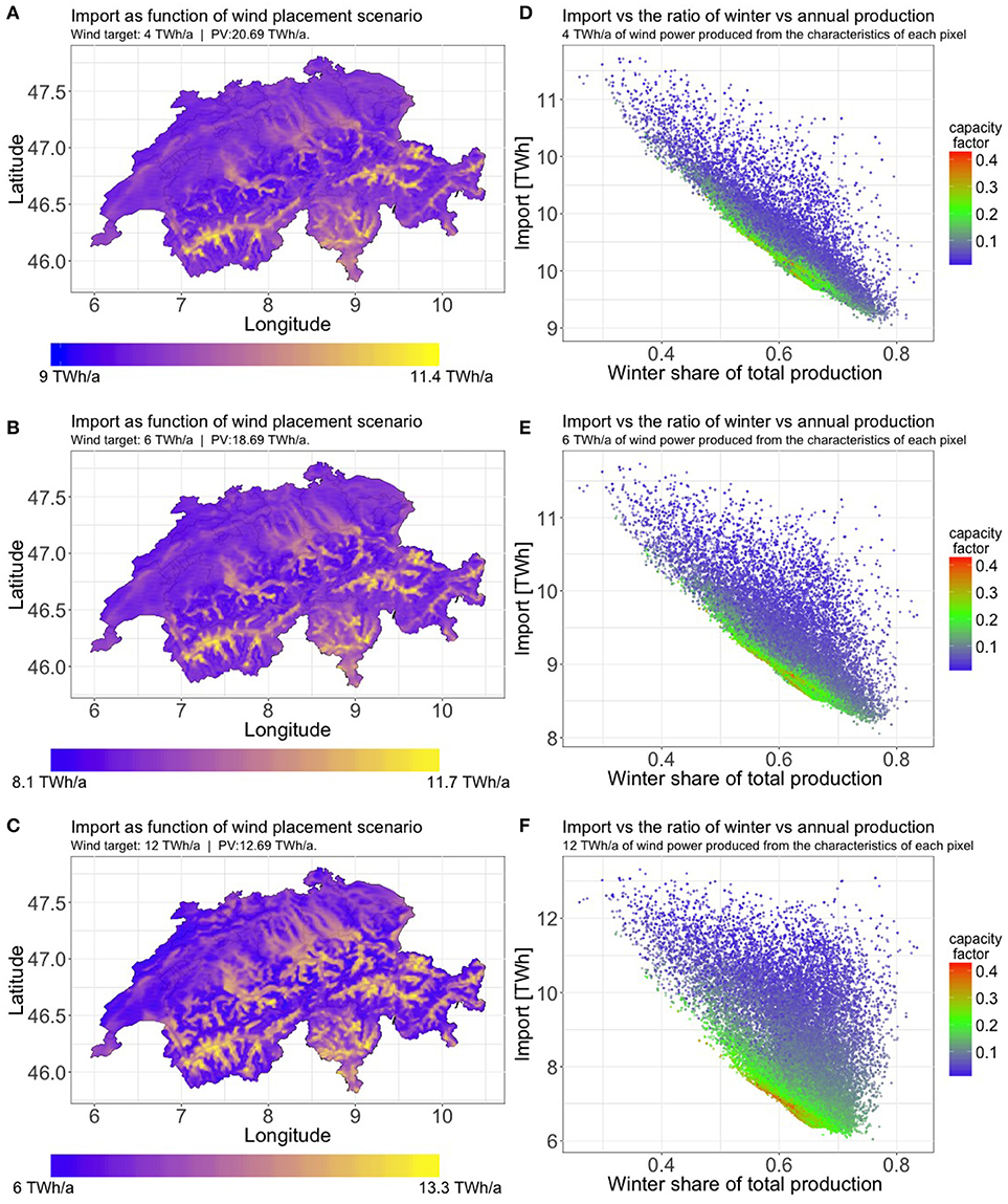
Figure 7. Left (A–C): Producing various annual wind power targets (4, 6, or 12 TWh/a) from the characteristic time series of each COSMO-1 pixel. The Import required to balance the system is plotted in each pixel. We can see a clear relation to the topography. Right (D–F): The relation between import and the share of total production that is produced in winter, for the same data as on the left. The highest capacity factors are found around the 60% winter production range. Each point in the plot represents the time series from a 0.01° pixel in the COSMO-1 dataset, scaled to produce 4, 8, or 12 TWh/a. Winter is defined as November through April.

We can look at these results in another way by plotting the resulting import as a function of the share of total production that is produced in the winter months. In the right side of Figure 7 this is done for the 3 wind targets of 4, 6, and 12 TWh/a. From these figures it becomes clear that the best producing wind locations (in terms of capacity factor) do not reduce import the most. Those locations that contribute most to low imports are the ones that produce most of their annual power during the winter months. In other words: in order to reduce the import the winter production needs to be as high as possible, relative to the total annual production (a high winter capacity factor relative to the annual capacity factor). Those locations that exhibit this behavior (the lower right corner of Figures 7D–F) unfortunately have low overall capacity factors, making them unattractive for wind power development. The feasible locations, i.e., the ones with high capacity factors, are the orange to red points. For increasing annual wind power targets from 4 TWh/a to 12 TWh/a, the resulting imports associated with these points goes down (compare the red points in Figure 7D with those in Figure 7F), showing that high shares of wind power in a renewable Swiss electricity supply lead to self-sufficiency with lower imports. This is in line with the findings in Dujardin et al. (2017).

One caveat should be placed however: In this section we have disregarded the capacity required to reach a wind power target. Therefore, in order to minimize imports, wind locations that produce high shares of their production in winter are favored, even if their total annual production is low, because we scale the production until the annual target is met. In reality, wind locations producing high absolute amounts of power will be the economically viable ones. Therefore, economically viable options that also reduce imports will be the ones producing both a high absolute amount of power as well as a large part of this in winter. Obviously, in a future electricity market without subsidies per kWh and with high amounts of PV, it remains to be seen what the market value of summer electricity will be, compared to that of winter electricity. In the next section, we will look at the required capacity to reach a certain target.

3.5. Required Number of Turbines

In this section we investigate the optimal placement of turbines across Switzerland, with the goal of minimizing the capacity required to produce a certain annual wind power target. In order to assess the influence of turbine siting on the required turbine capacity, the production of a bi-annual national production target from turbines with increasing elevation limits is simulated. Initially, the capacity to produce an annual wind power target of 6 TWh/a is assessed, while in a later section, higher and lower targets are explored. To improve robustness, the simulation is repeated 10 times for each elevation cap, as it involves a random selection of a pixel subset. Two cases are simulated. First, from this random subset, turbine locations are selected based on the highest annual capacity factor. Secondly, we have selected candidate locations based on the highest capacity factor in the winter months. The results are shown in Figure 8, where the capacity in MW required to produce 6 TWh of annual wind power is plotted as a function of the mean elevation of the locations used for wind power production in each scenario. Clearly visible is a downward trend in the required capacity with increasing mean elevation. This holds for both the cases where locations are selected based on annual capacity factor, as when they are selected based on winter capacity factor. An annual production target of 6 TWh/a could be achieved with as little as 1914 MW when turbines are located at a mean elevation of 2967 m.a.s.l. However, when we restrict the elevation, the required capacity increases as the maximum elevation at which we allow turbines to be sited decreases, up to 2454 MW for a maximum elevation of 1400 m.a.s.l. Obviously selecting the pixels with highest annual capacity factor (and thus production) will lead to the lowest capacity required to reach a certain annual target. However when we look at the resulting import, we see that selecting turbine locations based on winter capacity factor leads to a small but significant reduction in the resulting imports for the system. This becomes more clear when we plot the same data as a function of import (Figure 9). Apparently reducing imports (through wind turbine siting) comes at a cost of increased capacity if the same annual target is to be met. This is however partly a result of the separate PV and wind power targets. Reducing imports under a combined renewables target might lead to more wind power at the expense of PV, as we have seen in section 3.4, as well as in Dujardin et al. (2017).

FIGURE 8

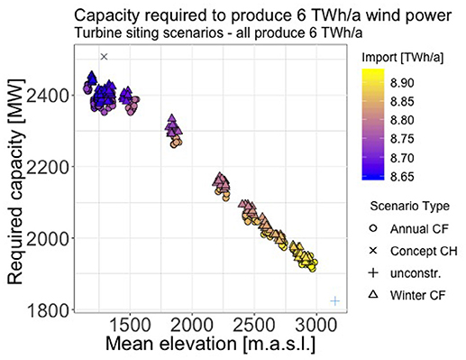
Figure 8. The required capacity as function of the mean elevation of the locations where turbines are located in each scenario. Also included in this figure are a scenario based on the Swiss Wind Energy Concept Bundesamt für Raumentwicklung (2017), “Concept CH,” as well as a scenario without constraints on elevation or locations (“unconstr”).

FIGURE 9

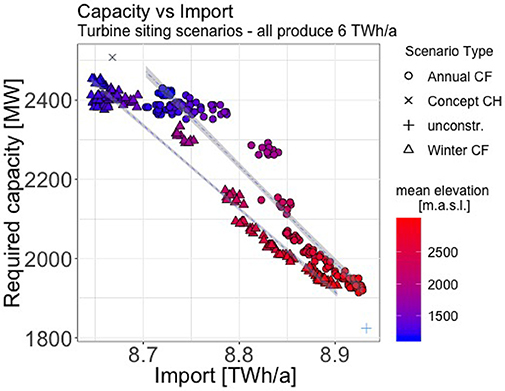
Figure 9. Various random subsets of the COSMO-1 pixels to reach 6 TWh/a wind power production. Also included in this Figure are a scenario based on the Swiss Wind Energy Concept Bundesamt für Raumentwicklung (2017), “Concept CH,” as well as a scenario without constraints on elevation or locations (“unconstr”). Two regression lines are shown, one for the elevation-dependent winter capacity factor scenario-set and one for the elevation-dependent annual capacity factor scenario-set.

3.6. Swiss Wind Energy Concept

We have also investigated the capacity required to produce 6 TWh/a when the potential turbine locations are constrained according to the Swiss Wind Energy Concept Bundesamt für Raumentwicklung (2017). Plotted in Figures 8, 9 is the siting scenario constrained by this policy document. From the locations described in the Swiss Wind Energy Concept, the best pixels (based on the annual capacity factor) have been selected and filled with 6 MW per pixel until the bi-annual target of 12 TWh (6 TWh/a) was reached. 2508 MW is required to reach this target. This can be compared to the unconstrained scenario, where the best pixels from the whole of Switzerland are selected without any limitations on elevation or number of candidate locations. This gives a theoretical best attainable solution of 1824 MW. It should be noted that all practical and logistic constraints are neglected in this latter case, as well as in the elevation dependent scenarios. Therefore, a direct comparison with the SwissWind Energy Concept scenarios does not hold.

3.7. Capacity as Function of Annual Wind Power Production

Although the dynamics are relatively similar for wind targets other than 6 TWh/a, in Figure 10 the capacities that are required for 4 and 12 TWh/a are also plotted, again as a function of mean turbine elevation. Where in Section 3.4 we speculated that for higher wind power targets it might be possible to achieve lower overall imports to balance the energy system on an annual basis, we can see in Figure 10 that this is indeed the case. What we however can also see, is that increasingly more capacity is required to produce additional wind energy. This can be explained from the fact that the best locations get used first, and increasingly less productive locations are used to produce additional output. As an example, the lowest capacity we found to produce 4 TWh/a is 1230 MW, whereas 6 TWh/a requires at least 1914 MW, which is more than a 150% increase.

FIGURE 10

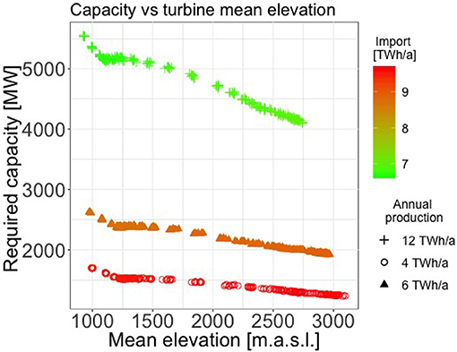
Figure 10. The required capacity as function of the mean elevation of the locations where turbines are located in each scenario, with scenarios for the 3 production targets of 4, 6, and 12 TWh/a.

3.8. Sensitivity to Wind Speed Errors

In this work, as in any modeling exercise, we have had to make a number of assumptions and simplifications that have an impact on the results. For one, the selection of an optimal wind turbine for a specific location can arguably increase the yield, something we have not incorporated in our approach. However the uncertainty in wind speeds is arguably more significant and has the highest influence on the results. To grasp the effects this may have, we have assessed how this translates to power output as follows: Since the power curve of a wind turbine is not a linear function of the wind speed, translating errors in wind speed measurement to power output is not straightforward. The power curve can be divided into four important sections: Below cut-in speed no power is produced, while between the cut-in speed and the rated speed the power output increases nonlinearly with the wind speed. Finally between rated and cut-out speed the power output is constant, until there is no power produced when wind speeds exceed the cut-out speed. In Figure 11 we have plotted the MBE for the COSMO-1 wind speeds in these three important operating ranges of the turbine used in this work, the Enercon E82, where we have translated the cut-in, rated, and cut-out speeds to the 10 m level via the log law, as described in Kruyt et al. (2017). We can see that in the nonlinear part of the power curve, between cut-in and rated speed, the bias is small with −0.4 m/s. For the speeds below cut-in, we have a positive bias of 1.65 m/s. This tells us that on average, our model set up will produce small amounts of power at low wind speeds that a turbine at that location would not produce. However, since this will be at the bottom of the nonlinear part of the power curve, these effects can be expected to be small. Finally at the top end of the power curve is where we see a large negative bias of −2.74 m/s. This tells us that our modeled power output will on average (over all stations) be lower than in reality.

FIGURE 11

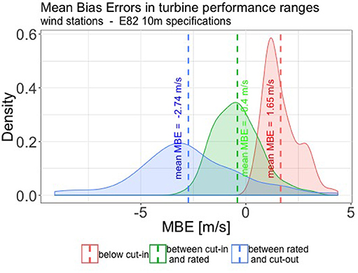
Figure 11. MBE for turbine performance ranges.

4. Conclusions

4.1. Wind Resource Assessment With COSMO-1

In this paper a series of calculations have been presented investigating the dynamics of a highly renewable Swiss power system with a focus on the role of wind energy. We have used the COSMO-1 model to this end, after assessing its performance in complex terrain with regards to hourly wind speeds. Although the RMSE for wind exposed locations in the Swiss Alps is still significant with a RMSE of 2.87 m/s, the MAE of (bi-)annual mean speeds is lower than previous works (at 0.83 m/s compared to 1.5 m/s reported in the wind atlas (Koller and Humar, 2016)), as well as more robust given the high number of stations used in our validation. Moreover, to our knowledge it is the first time wind resource assessment for the complex terrain of the Swiss Alps is based on a fully physical model, rather than using statistics to correlate static wind fields to topography. COSMO-1 systematically overestimates wind speeds at sheltered stations of the IMIS network, but since these locations are chosen to be relatively sheltered, this bias may be more due the location and not representative of the entire 0.01° grid cell. For wind exposed stations, bias is almost zero. Analysing the bias for the ranges of speeds that correspond to the different linear and non-linear sections of the turbine's power curve, we estimate that the error in the wind speed likely leads to a slight underestimation of overall power simulations. However we also ignore forced outage due to maintenance and icing, which likely overestimates results.

4.2. Import Reduction and Wind Power

Next, the wind speeds from the COSMO-1 model were used to produce time series for wind power production. We then used these power time series in a spatially aggregated model of the Swiss electricity system to investigate the influence of wind turbine locations on the power system. We have conducted a series of simulations where increasing amounts of wind power were produced from the characteristic wind time series of single locations in Switzerland. We've used the resulting power time series in a model of the Swiss electricity system where we simulate a renewable Swiss power supply. This has shown us that for a hypothetical, fully renewable Swiss power system, the higher the share of wind power in the renewable electricity mix, the lower the resulting imports can be. This crucially depends on the turbine's locations however, since there are large differences in wind climate across Switzerland. The turbine locations that contribute most to import reduction are those with high production during the winter months. This shows that wind power has to be a key element in a future renewable Swiss power supply, if a heavy dependence on imports is to be avoided.

4.3. Required Capacity

We have investigated the capacity that is required to reach a certain annual wind target, and how the siting scenarios influence overall system parameters such as the import required to balance the system. As with any modeling exercise of complex real world phenomena, there are a number of simplifications and assumptions that call for somewhat cautious interpretation of the exact values. However, since the focus of this work has been on the dynamics of the energy system, the following conclusions can be drawn from our results:

For an annual wind power production of 6 TWh/a, the theoretical minimum amount of capacity required to produce this target is 1824 MW. This neglects all practical and political restraints on turbine siting, and should be seen as a rather theoretical limit more than a practical goal. However, it does give a sense of scale to the rest of the results. Because for further simulations, turbines have been located at different elevations to achieve an annual target. Here we found a strong relation between the mean elevation of the turbine locations and the required capacity to reach that goal. Increasing the mean elevation of turbine locations from 1189 m.a.s.l. to 2967 m.a.s.l. leads to a 28.2 % reduction in the capacity that is required to produce 6 TWh/a of wind power. For the often mentioned Swiss wind power target of 4 TWh/a in 2050, we calculate the minimal capacity to reach this to be 1230 MW. But also here, this requires turbines to be built at high elevations.

These results call for a focus on high elevation wind power in the planning and development of wind power capacity. Transitioning away from nuclear power toward a renewable electricity supply will prove a daunting task, and as such it is imperative to do so in the most space- and cost efficient manner. Our results show that high-elevation wind power can form a crucial element in achieving the Energy Strategy 2050 wind power target with minimal capacity. In Switzerland, public opposition against wind turbines in mountains appears significant. However, the ‘Energy Strategy 2050' was accepted in a 2017 referendum (Bundesrat, 2017) and previous research shows that generally, Swiss people are accepting of wind energy (Jegen, 2015). That same research however also cites the multi-level decentralization, sectoral policies with diverging objectives and high population density as reasons for the slow increase in wind power capacity in Switzerland. As land-use conflicts as well as population density are arguably fewer at high elevations, focussing efforts on high elevation wind power may also minimize conflicts in these domains.

Our modeling approach has been focussed on minimizing the capacity to reach an annual goal, and as such not well suited for other optimisation goals. However, scenarios where capacity was located based on highest winter capacity factor rather than the annual capacity factor did achieve a slight decrease in overall imports required to balance the system.

4.4. Outlook

Although we have managed to qualitatively assess the effects that uncertainties in wind speed may have on power estimates, reducing the RMSE in the modeled wind speeds would be an important step forward. Given the scales of the topography, this most likely implies an increase in horizontal modeling resolution. Given the increase in computational burden this entails, it is more feasible to simulate small areas of interest than the whole of Switzerland. Such areas should be pre-selected based on lack of spatial planning conflicts, logistic feasibility and initial potential assessments. As is the case with any wind farm development project, after initial site identification which may be based on the work in this paper, various steps such as those described in section 2.5 will need to be undertaken at the individual site level before a wind farm may actually be developed.

Further integration of resource and electricity models may allow for more complex optimisation problems. We have now looked at turbine locations and their effects on the capacity required to reach a certain target, but it may be more insightful to analyse the combined optimal siting of both PV and wind, with the objectives of minimizing both required capacity and resulting system imports. Our current set up with separate targets for wind and PV production does not allow for this. Combining such strategies with optimal wind siting strategies in a power flow model will be the next step toward a better understanding of a fully renewable and efficient Swiss power system.

All land-use and spatial planning concerns that may limit areas for wind turbines to be build have been ignored in this study, except for the scenario based on the Swiss Wind Energy concept, which by definition includes such considerations. Caution should therefore be taken in comparing these numbers directly to our idealized scenarios. We have also ignored all logistical limitations of building wind turbines at high elevations. It may very well be technically near impossible, or at least very costly, to build turbines at some of the high elevation locations we used in this study. A study into the economical wind potential for Switzerland could include such effects, possibly by incorporating a cost function based on the inverse distance to roads or other infrastructure to take into account the additional cost of high elevation wind power in remote locations. The downside of economic potential assessment is that it is heavily dependent on current prices and subsidies of not only the technology in question, but also those of competing ones, making the relevance of the results very short-lived. Moving the current work forward toward a geographical/political potential assessment (see section 2.5) will be a complex task, given the decentralized and layered structure of Swiss governance. While federal considerations have been accounted for in the ‘Swiss wind energy concept' (Bundesamt für Raumentwicklung, 2017), at the cantonal and municipality level there is little information available. We hope that this work will at least lead to better awareness of the potential, and prompt a structured mapping of other land-use and political interests at various political levels, which will be the next step in moving a national wind energy potential assessment forward.

Data Availability

The datasets generated for this study can be found on envidat https://www.envidat.ch/dataset/dataset-onwind-fields-and-energy-potential-in-swiss-alps with the doi: 10.16904/envidat.51.

Author Contributions

BK was responsible for the research (concept, methodology, application, conclusions, writing), JD developed the aggregated electricity model and provided feedback on use and research set-up. ML supervised the project and provided input on the research concept and methodology.

Conflict of Interest Statement

The authors declare that the research was conducted in the absence of any commercial or financial relationships that could be construed as a potential conflict of interest.

Acknowledgments

This research is funded by the Swiss National Science Foundation under the National Research Programme NRP 70 ‘Energy Turnaround', and Innosuisse (SCCER-SoE). It would not have been possible without the cooperation and excellent infrastructure from both MeteoSwiss and The Swiss National Supercomputing Centre CSCS (the latter under project s569). We would further like to thank Christoph Marty, Benoit Gherardi and Michel Bovey for their help with the data acquisition, and Annelen Kahl for supplying irradiance data and PV modeling methodology.

Footnotes

1. ^Current Swiss electricity demand is about 62 TWh/a (Bundesamt für Energie BFE, 2017).

2. ^Koller and Humar (2016) write they report the error of a ‘representative location' for a landscape type (i.e., mountain, valley etc.)

3. ^personal communication with major Swiss wind power developer

References

Bundesamt für Energie (BFE) (2017). Schweizerische Elektrizitätsstatistik 2016. Technical report, Bundesamt für Energie BFE.

Abhari, R., Andersson, G., Banfi, S., Bébié, B., Boulouchos, K., Bretschger, L., et al. (2012). Zukunft Stromversorgung Schweiz. Technical report, Akademien der Wissenschaften Schweiz (Bern).

ADB, A. D. B. (2014). Guidelines for Wind Resource Assessment Best Practices for Countries Initiating Wind Development. 1–49. Available online: https://www.adb.org/sites/default/files/publication/42032/guidelines-wind-resource-assessment.pdf

Ayuso, M., and Kjaer, C. (2016). World Energy Resources Wind — 2016. World Energy Council 71.

Barber, S., Chokani, N., and Abhari, R. S. (2011). Assessment of wind turbine performance in alpine environments. Wind Eng. 35, 313–328. doi: 10.1260/0309-524X.35.3.313

CrossRef Full Text | Google Scholar

Bauer, C., Hirschberg, S., Bäuerle, Y., Biollaz, S., Calbry-Muzyka, A., Cox, B., et al. (2017). Potentials, Costs and Environmental Assessment of Electricity Generation Technologies. Technical report, Bundesamt für Energie BFE Sektion Energieversorgung und Monitoring Potentials (Bern).

Berge, E., Gravdahl, A. R., and Schelling, J. (2006). “Wind in complex terrain. A comparison of WAsP and two CFD-models,” in European Wind Energy Conference and Exhibition 2006, EWEC 2006 (Athens).

Google Scholar

Brugger, E. A., Dietrich, P., Gessler, R., Giger, K., Hofstetter, P., Kaiser, T., et al. (2009). Erneuerbare Energien : übersicht über vorliegende Studien und Einschätzung des Energie Trialog Schweiz zu den erwarteten inländischen Potenzialen für die Strom-, Wärme- und Treibstoffproduktion in den Jahren 2035 und 2050 inklusive Berücksichtigung der P. Trialog.

Bundesamt für Energie BFE (2017). Schweizerische Elektrizitäts Statistik 2017. Technical report, Bundesamt für Energie BFE.

Bundesamt für Energie BFE and Bundesamt Für Umwelt, W. u. L. B. B. F. R. A. (2004). Konzept windenergie Schweiz. Technical report, Bundesamt für Energie BFE (Bern).

Bundesamt für Energie BFE und Landschaft, B. F. U. W., and Are, B. F. R. (2004). Konzept Windenergie Schweiz-Methode der Modellierung Geeigneter Windpark-Standorte. Technical report, Bundesamt für Energie BFE, Bern.

Bundesamt für Raumentwicklung (2017). Konzept Windenergie. Sachpläne und Konzepte, 33. Available online at: www.bundespublikationen.admin.ch

Bundesrat, S. F. C. (2017). Energy Act (EnA). Available on;line at: https://www.admin.ch/gov/en/start/documentation/votes/Popular vote on 21 Mai 2017/Energy-Act.html

Consortium for Small-scale Modeling (2017). COSMO Model. Available online at: http://www.cosmo-model.org

Denholm, P., Hand, M., Jackson, M., and Ong, S. (2009). Land-Use Requirements of Modern Wind Power Plants in the United States Land-Use Requirements of Modern Wind Power Plants in the United States. National Renewable Energy Laboratory, Technical(August):46.

Dierer, S., Remund, J., Schaffner, B., Stauch, V., and Hug, C. (2009). “Wind power predictions for Switzerland: the performance of different downscaling methods for complex terrain,” in 2009 European Wind Energy Conference and Exhibition.

Draxl, C., and Mayr, G. J. (2011). Meteorological wind energy potential in the Alps using ERA40 and wind measurement sites in the Tyrolean Alps. Wind Energy 14, 471–489. doi: 10.1002/we.436

CrossRef Full Text | Google Scholar

Dujardin, J., Kahl, A., Kruyt, B., Bartlett, S., and Lehning, M. (2017). Interplay between photovoltaic, wind energy and storage hydropower in a fully renewable Switzerland. Energy 135, 513–525. doi: 10.1016/j.energy.2017.06.092

CrossRef Full Text | Google Scholar

Federal Department of the Environment Transport Energy Communications DETEC (2018). DETEC-Energy Strategy 2050. Available online at: https://www.uvek.admin.ch/uvek/en/home/energy/energy-strategy-2050.html

Grünewald, T., Dierer, S., Fundel, F., and Lehning, M. (2012). Mapping frequencies of icing on structures in Switzerland. J. Wind Eng. Ind. Aerodyn. 108, 76–82. doi: 10.1016/j.jweia.2012.03.022

CrossRef Full Text | Google Scholar

Helbig, N., Mott, R., Van Herwijnen, A., Winstral, A., and Jonas, T. (2017). Parameterizing surface wind speed over complex topography. J. Geophys. Res. 122, 651–667. doi: 10.1002/2016JD025593

CrossRef Full Text | Google Scholar

Hirschberg, S., Bauer, C., Burgherr, P., Biollaz, S., Durisch, W., Foskolos, K., et al. (2005). Neue Erneuerbare Energien und neue Nuklearanlagen: Potenziale und Kosten. Technical Report 05, Paul Scherrer Institut PSI (Villigen).

Hoogwijk, M., de Vries, B., and Turkenburg, W. (2004). Assessment of the global and regional geographical, technical and economic potential of onshore wind energy. Energy Econ. 26, 889–919. doi: 10.1016/j.eneco.2004.04.016

CrossRef Full Text | Google Scholar

Hoogwijk, M., and Graus, W. (2008). Global Potential of Renewable Energy Sources: A Literature Assessment. Background report prepared by order of ….

Jafari, S., Sommer, T., Chokani, N., and Abhari, R. S. (2012). “Wind Resource Assessment Using a Mesoscale Model: The Effect of Horizontal Resolution,” in Proceedings of ASME Turbo Expo 2012 GT2012 June 11-15, 2012, Copenhagen, 987.

Google Scholar

Jegen, M. (2015). “Energy transition and challenges for wind energy in Switzerland,” in Climate Change and Renewable Energy Policy Workshop, Carleton University, 2–6.

Koller, S., and Humar, T. (2016). Windpotentialanalyse für Windatlas.ch: Jahresmittelwerte der modellierten Windgeschwindigkeit und Windrichtung. Schlussbericht. Technical report, MeteoTest, BFE.

Kruyt, B., Lehning, M., and Kahl, A. (2017). Potential contributions of wind power to a stable and highly renewable Swiss power supply. Appl. Energy 192, 1–11. doi: 10.1016/j.apenergy.2017.01.085

CrossRef Full Text | Google Scholar

Lehning, M., Bartelt, P., Brown, B., Russi, T., St??ckli, U., and Zimmerli, M. (1999). SNOWPACK model calculations for avalanche warning based upon a new network of weather and snow stations. Cold Reg. Sci. Technol. 30, 145–157. doi: 10.1016/S0165-232X(99)00022-1

CrossRef Full Text | Google Scholar

Leuenberger, D., Koller, M., Fuhrer, O., and Schär, C. (2010). A generalization of the SLEVE vertical coordinate. Mon. Weather Rev. 138, 3683–3689. doi: 10.1175/2010MWR3307.1

CrossRef Full Text | Google Scholar

Lewis, H. W., Mobbs, S. D., and Lehning, M. (2008). Observations of cross-ridge flows across steep terrain. Q. J. R. Meteorol. Soc. 134, 801–816. doi: 10.1002/qj.259

CrossRef Full Text | Google Scholar

Mayr, G. J., Armi, L., Gohm, A., Zangl, G., Durran, D. R., Flamant, C., et al. (2007). Gap flows: results from the mesoscale alpine programme. Q. J. R. 133, 937–948. doi: 10.1002/qj

CrossRef Full Text | Google Scholar

Meyers, J., and Meneveau, C. (2012). Optimal turbine spacing in fully developed wind farm boundary layers. Wind Energy 15, 305–317. doi: 10.1002/we.469

CrossRef Full Text | Google Scholar

Prognos (2012). Die Energieperspektiven für die Schweiz bis 2050. Technical report, Bundesamt für Energie BFE.

Schaffner, B. and Remund, J. (2005). ALPINE WINDHARVEST Report 7-2: Modeling Approach. Technical Report April 2005, MeteoTest, Bern.

Schär, C., Leuenberger, D., Fuhrer, O., Lüthi, D., and Girard, C. (2002). A new terrain-following vertical coordinate formulation for atmospheric prediction models. Mon. Weather Rev. 130, 2459–2480. doi: 10.1175/1520-0493(2002)130h2459:ANTFVCi2.0.CO;2

CrossRef Full Text | Google Scholar

Sharma, V., Cortina, G., Margairaz, F., Parlange, M. B., and Calaf, M. (2018). Evolution of flow characteristics through finite-sized wind farms and influence of turbine arrangement. Renewable Energy 115, 1196–1208. doi: 10.1016/j.renene.2017.08.075

CrossRef Full Text | Google Scholar

SLF (2016). Measurement and Information System (IMIS). Available online at: http://www.slf.ch/ueber/organisation/warnung_praevention/warn_informationssysteme/messnetze_daten/imis/index_EN

Truhetz, H. (2010). High Resolution Wind Field Modelling Over Complex Topography : Analysis and Future Scenarios. Ph.D. thesis, Graz.

Truhetz, H., Krenn, A., Winkelmeier, H., Müller, S., Cattin, R., Eder, T., and Biberacher, M. (2012). “Austrian wind potential analysis ( AuWiPot ),” in 12. Symposium Energieinnovation, 15.-17.2.2012, Graz/Austria, 1–10, (Graz).

Google Scholar

VSE (2014). Basiswissen Windenergie. Technical Report September 2013, Verband Schweizer Elektrizitätsunernehmen VSE.

Williams, A. (2014). Improving Wind Farm Availability Better Performance and Increased ROI Through Accurate Availability Measurement Improving Wind Farm Availability.

WindSim (2018). WindSim. Available online at: https://windsim.com/

Winkelmeier, H., Krenn, A., and Zimmer, F. (2014). Das Realisierbare Windpotential Österreichs für 2020 und 2030. Technical report, FFG Österreichische Forschungsförderungsgesellschaft mbH.

Winstral, A., Jonas, T., and Helbig, N. (2016). Statistical downscaling of gridded wind speed data using local topography. J. Hydrometeorol. doi: 10.1175/JHM-D-16-0054.1. [Epub ahead of print].

CrossRef Full Text | Google Scholar