 Xiaomeng Dong
 Zhijian Zhang1*
95% of researchers rate our articles as excellent or good
Learn more about the work of our research integrity team to safeguard the quality of each article we publish.
Find out more
ORIGINAL RESEARCH article
Front. Energy Res. , 03 July 2018
Sec. Nuclear Energy
Volume 6 - 2018 | https://doi.org/10.3389/fenrg.2018.00058
This article is part of the Research Topic Nuclear Thermal Hydraulic and Two-Phase Flow View all 13 articles
Numerical simulation has been widely used in nuclear reactor safety analyses to gain insight into key phenomena. The Critical Heat Flux (CHF) is one of the limiting criteria in the design and operation of nuclear reactors. It is a two-phase flow phenomenon, which rapidly decreases the heat transfer performance at the rod surface. This paper presents a numerical simulation of a steady state flow in a vertical pipe to predict the CHF phenomena. The detailed Computational Fluid Dynamic (CFD) modeling methodology was developed using FLUENT. Eulerian two-phase flow model is used to model the flow and heat transfer phenomena. In order to gain the peak wall temperature accurately and stably, the effect of different turbulence models and wall functions are investigated based on different grids. Results show that O type grid should be used for the simulation of CHF phenomenon. Grids with Y+ larger than 70 are recommended for the CHF simulation because of the acceptable results of all the turbulence models while Grids with Y+ lower than 50 should be avoided. To predict the dry-out position accurately in a fine grid, Realizable k-ε model with standard wall function is recommended. These conclusions have some reference significance to better predict the CHF phenomena of vertical pipe. It can also be expanded to rod bundle of Boiling Water Reactor (BWR) by using same pressure condition.
Critical Heat Flux (CHF) is a two-phase flow phenomenon that is characterized by a heat transfer mechanism change which rapidly decreases the efficiency of the heat transfer performance at the heater surface. When it occurs, heated surfaces are no longer wetted by boiling liquid and the vapor phase start to occupy the heat surface. As a result, the energy is directly transferred from the heat surface to vapor. It results in rapid reduction of the heat removal ability and sharp rise of the vapor temperature, as well as the rod surface temperatures which are important for the nuclear safety. During the design and operation of the nuclear reactors, CHF value should be calculated in advance. But experience and thousands of data points have shown the complexity of CHF phenomenon for different conditions. In the past decades, both experiment and numerical simulation are widely used to predict the CHF value during the design and operation process. During the experimental process, the wall temperature is monitored by use of thermocouples. Along with the increasing of heat power, CHF phenomenon is detected when the temperature of one thermocouple has a sharp rise. Similar to the experiment, this sharp rise of the wall temperature is also a signal of CHF in the numerical simulation. So it is of great significance to predict the wall temperature accurately and stably.
Nowadays, experimental method is widely used in the CHF prediction. But most of them are focused on the vertical pipe. Large scale experiments of rod bundle are few reported or open-access around the world. In the reactor design area, CHF look-up table is the main method to determine the CHF value. But both these two methods will give a large safety margin, and then reduce the power level. Compared to experimental measurements and CHF look-up table, numerical simulation has its own advantages. Thermal-hydraulics system or subchannel codes can efficiently characterize bulk flow behavior, while computational fluid dynamics (CFD) analysis may provide relatively accurate results for the velocity and temperature profiles around the rods. Although the subchannel analysis is more widely used for CHF prediction, CFD method can work as a supplement to provide more accurate results. Furthermore, numerical simulation can reduce the cost significantly when we use different geometries, materials, and test conditions. More accurate simulation techniques using these combined analysis tools can be used to optimize experimental designs and improve the test-analysis design cycle for advanced fuel rods.
Grids and turbulence models are found to be very important in the Computational Fluid Dynamic (CFD) simulation. At the moment, turbulence models used in two phase flow are still same with that of single phase flow. Especially in Eulerian two phase model, the liquid and vapor phases are applied with same turbulence model separately. In single phase flow, the results of Chen et al. (2017a) show different turbulence models will deliver to different secondary flow status. This conclusion is more obvious for isotropic and anisotropic turbulence models. However, the conclusion about applicability of these turbulence models is not consistent for the simulation of two phase flow. Standard k-ε model has been chosen by some researchers for its stability on the two phase calculation. Shin and Chang (2009) has used this model to study the effect of mixing vane on CHF enhancement by use of two-fluid model. It is also used by Shirvan (2016) to study the boiling crisis at high pressures. Shirvan's Results show same trend with the Russian CHF data at the condition close to Departure of Nucleate Boiling (DNB). In addition, a new mechanistic model was developed by Mimouni et al. (2016) to predict CHF in boiling flow of water and R12 refrigerant by use of k-ε models in Neptune-CFD code. Mimouni's results are compared with 150 tests and the mean relative error is equal to 8.3%. Apart from standard k-ε model, Shear Stress Transport (SST) k-ω model is also used by some researchers. Krepper et al. (2007, 2013) and Krepper and Rzehak (2011) predicted the subcooled boiling process in vertical heated tubes with water and R12 based on the SST k-ω turbulence model. Subcooled boiling flow in Internal Combustion (IC) engine cooling passages was studied based on SST k-ω turbulence model (Hua et al., 2015). The simulation results showed that present two-fluid model could get an accurate temperature field for cylinder head.
Although different turbulence models are used for the calculation of two phase flow, few researchers has ever compared the effect of different grids and turbulence models. In general, a grid dependency study should always be performed in high quality CFD simulation. Even though it is hard to obtain fully grid independent results in some cases, it is necessary to discuss the effect of key grid parameters. Thakrar et al. (2016) has investigated the nucleate boiling in rectangular geometries at high pressure by use of CFD code STAR-CCM+. Standard k-ε model and Reynolds Stress Transport models were compared to investigate the influence of turbulence. Results show the most mechanistic configurations produced remarkably good agreement with measurements of the area-averaged void. But the grid-dependent wall treatments are still needed to develop. Zhang et al. (2015) has analyzed the effect of grids and turbulence models for subcooled boiling flow in a vertical pipe. Her results show that the turbulence models could be chosen appropriately according to the Y+. This paper shows a relatively overall investigation for the options of grids and turbulence models in the subcooled boiling flow.
However, as we can see above, few researchers have ever shown the sensitivity analysis on turbulence models and wall functions for CHF phenomenon. The grid dependency study is also ignored in the CFD simulation of boiling two-phase flow, especially on the CHF phenomenon. It is still not clear that if the turbulence models have the same performance on CHF phenomena as that of subcooled boiling flow, especially on the value and position of highest wall temperature. So based on Eulerian two-phase model, this paper presents numerical simulations of CHF phenomenon by the use of CFD method to investigate the effect of different grids, turbulence models and wall functions. Lack of open CHF experimental data of rod bundle, especially the wall temperature distribution, we use vertical pipe instead. Considering both the flows in rod bundle and vertical pipe are vertical upward flow, the flow and heat characteristics are similar to each other as long as we use same pressure condition. The type of boiling crisis is dryout which can be identified by the distribution of wall temperature and void fraction. Results are focused on the wall temperature distribution to give a reference for the detector of CHF phenomena.
Eulerian two-phase models are used as the basic models to simulate the two phase flow in a vertical pipe. All the interfacial mass, momentum and energy transfer models are based on the interfacial area density model. Furthermore, CHF model will also be shown below.
The conservation equation of Eulerian two phase model includes six equations which are mass, momentum and energy equations for two phases separately. These six equations will be solved for six parameters which include pressure, velocities of liquid and vapor, temperatures of liquid and vapor, volume fraction.
(1) Mass equations
(2) Momentum equations
(3) Energy equations
Where α,ρ,v,S, p,τ, g, and h refer to volume fraction, density, velocity, source term, pressure, stress-strain tensor, gravity and specify enthalpy. m and Q are the interfacial mass and energy transfers from phase v to phase l. The force F includes five parts, FD, Flift, Fwl, Fvm, Ftd. They are the drag force, lift force, wall lubrication force, virtual mass force and turbulence dispersion force which will be introduced in detail respectively.
The interfacial momentum transfers between liquid and vapor phases are decided by the five forces which are the drag force, lift force, wall lubrication force, virtual mass force and turbulence dispersion force.
For fluid-fluid flow, each secondary phase is assumed to form droplets or bubbles. This assumption gives a method to derivate the drag force which is the most important force of these five parameters. Drag force refers to the force that droplets or bubbles suffer because of the different velocities. As we know, because of viscosity, the general form of the drag force is:
When it is used for a particle in the fluid, this form will be changed to
Where A is the projected area of the particle, ρl is the density of the continuous phase, Vl and Vv are the velocities of different phase. CD is a coefficient. For the droplets or bubbles, A can be expressed as , where d is the diameter.
Associated with Re number whose form is
We can gain a new form of drag force of the droplets or bubbles which is
So in per unit mixture volume, the drag force can be expressed as
Where is always called drag force coefficient which is estimated by Ishii model (Ishii, 1979). is called particulate relaxation time. is the interfacial area concentration which is an important value.
Lift force act on a particle mainly due to velocity gradients in the continuous phase flow field. It is calculated by the function from Drew and Lahey (1993).
In this equation, Clift is the lift force coefficient provided by Moraga model (Moraga et al., 1999). This model is applicable mainly to the lift force on spherical solid particles, though it can be applied to liquid drops and bubbles.
Wall lubrication force which tends to push the bubbles away from the wall can be expressed as
Where is the phase relative velocity component tangential to the wall surface, and nw is the unit normal pointing away from the wall. The coefficient Cwl is calculated by Antal Model (Antal et al., 1991).
Virtual mass effect should be included when the secondary phase accelerates relative to the primary phase. It is defined as
The turbulent dispersion force acts as a turbulent diffusion in dispersed flows. It plays an important role in driving the vapor away from the vicinity of the wall to the center of the channel. Bertodano (1991) proposed the following formulation:
Where CTD is a constant, it is equal to 1 by default in the following calculation.
The interfacial energy transfers includes two parts which are the heat from liquid to vapor phase at the near wall region and the heat transfer between vapor and liquid phases in the subcooled bulk. As the bubbles depart from the wall and move to the subcooled region, there is heat transfer from the bubble to liquid that is defined as
The heat transfer coefficient can be computed using Ranz and Marshall (1952) model.
The interface to vapor heat transfer is calculated using the constant time scale return to saturation method which was provided by Lavieville et al. (2005). It is assumed that the vapor retains the saturation temperature by rapid evaporation and condensation. The formulation is
In this equation, δt is the time scale.
Depends on the theory, interfacial mass transfer can also be divided in to two parts: liquid evaporation near the wall and liquid evaporation or vapor condensation in the main stream. The former is calculated on the basis of evaporation heat flux which will be introduced below.
The latter can be calculated directly based on the interfacial energy transfer and latent heat hfv.
Different from the heat transfer of single phase flow on the near wall region, the heat transfer of two-phase flow includes three different types heat transfer. As we can see from the subcooled boiling flow, the energy is transferred directly from the wall to the liquid. Part of this energy named convective heat flux will cause the temperature of the liquid to increase and part which is called evaporative heat flux will generate vapor. Interphase heat transfer will also cause the average liquid temperature to increase; however, the saturated vapor will condense. In addition, there is a quenching heat flux which model the cyclic averaged transient energy transfer related to liquid filling the wall vicinity after bubble detachment. These basic mechanisms are the foundations of the Rensselaer Polytechnic Institute (RPI) models developed by Kurul and Podowski (1991).
To model boiling departing from the nucleate boiling regime, or to model it up to the critical heat flux and post dry-out condition, it is necessary to include the vapor temperature in the solution process. In such cases, some of the energy may be transferred directly from the wall to the vapor. So in total, the wall heat partition will be expressed as
The four heat fluxes qC, qQ, qE, qV is defined as
Where TW, Tl, TV are the temperature of the wall, liquid and vapor. hC and hV are the heat transfer coefficient. kl is the thermal conductivity. is the diffusivity. hfv is the latent heat of evaporation. ρv is the vapor density. Vd is the volume of the bubble based on the bubble departure diameter Dw. T is the periodic time. Ab is the area of influence which is covered by nucleating bubbles. Nw is the nucleate site density.
The nucleate site density Nw is usually represented by a correlation based on the wall superheat.
The empirical parameters C = 210 and n = 1.805 are from Lemmert and Chawla (1977) model.
The bubble departure diameter Dw means the maximum diameters of bubbles when bubbles leave the wall. The empirical correlation is given by Tolubinski and Kostanchuk (1970).
The area of influence Ab is based on the departure diameter and the nucleate site density.
The coefficient K is given by Del Valle and Kenning (1985).
The last parameter is the frequency of bubble departure . In general, the bubble in the wall suffers three forces, which are buoyancy force, surface tension and drag force. When the heat flux is high and bubbles are large, the surface tension could be ignored. So according to the equilibrium of buoyancy force and drag force which was described in paper (Cole, 1960).
Associated with u = fDw and FD = 1, f can be expressed as.
In the model, the critical heat flux is defined to occur when the volume fraction of vapor reach given values which is provided by Tentner et al. (2006).
Where αv, 1 = 0.9 and αv, 2 = 0.95.
The numerical analysis is performed using the commercial CFD code FLUENT 16.0 (Ansys Fluent, 2015) which is part of ANSYS WORKBENCH 16.0. The modules we use are based on the finite volume method, and uses RANS (Reynolds averaged Navier-Stokes) equations for the solution of mass, momentum, energy and turbulence model.
CHF experiment data in an upward flow vertical pipe from Becker (1983) are used to validate the simulation method. Although there are much data in the Becker's experiment, one case with 7Mpa pressure which is condition of boiling water reactor (BWR) is investigated about the effect of grids and turbulence models. The facility has a 7m long heated pipe and the inner diameter is 10mm. Detail information about boundary condition are shown in Figure 1.
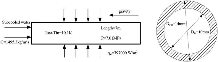
Figure 1. Geometry and boundary condition.
It has been tested that the grid type has limit influence on the temperature distribution in the single-phase flow (Chen et al., 2017b). But in two-phase flow, this conclusion is doubtful for the complexity of wall boiling status. So the effect of different grid type should be tested first before the investigation of turbulence models. As we can see from Figure 2, O type grid, arbitrary Hexaprism type grid and Triprism grid are calculated under the same boundary condition. Results are shown in section Effect of Grid Type.
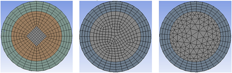
Figure 2. O type grid, arbitrary Hexaprism grid and Triprism grid.
All the turbulence models can be divided into high Reynolds and low Reynolds turbulence models according to its application. The standard k-ε model (Launder and Spalding, 1972) is typical high Reynolds turbulence model. It should be used for fully developed turbulence and isotropic flow. Because of its reduced computational complexity, it has been widely used for decades of years. An important weak point is that the standard k-ε model cannot deal with rotational flow or flow in curved pipe. To solve these problems, RNG (Re-Normalization Group) k-ε model (Yakhot and Orszag, 1986) and Realizable k-ε model (Shih et al., 1995) are developed in 1986 and 1995 separately. These two models expanded the application of k-ε model to a larger field. The secondary flow status of shear flow and rotational flow could be predicted to a certain extent. The k-ω models are low Reynolds turbulence model which have a larger application. The standard k-ω model (Wilcox, 1998) is more suitable for wall limited flow and free shear flow. In SST (Shear Stress Transport) k-ω model (Menter, 1994), the effect of turbulent shear force is included when solve the turbulent viscosity. It is also worth to note that SST k-ω model is same as standard k-ω model in near wall region and similar to standard k-ε model in the fully turbulent region.
The turbulence model should be used with suitable wall function or resolve the boundary layer with a fine-enough mesh without any wall functions. As we know, the near-wall region can be subdivided into three sublayers, i.e., viscous sublayer, buffer layer and fully turbulent region (Pope, 2000). For k-ε model with standard wall function, it uses an empirical correlation to solve the equations in viscous sublayer and buffer layer. It also requires the first node should be located in fully turbulent region where viscosity is of less effect. So according to reference (Pope, 2000), Y+ larger than 30 is recommended for high Reynolds turbulence models to ensure accuracy and stability. However, the enhanced wall function maybe helpful to use high Reynolds turbulence model in the region where Y+ is smaller than 30. The results sometimes show good agreement with experiment data. For k-ω model, it is essential to ensure the viscous sublayer to be covered with several cells to maintain the near wall Y+ to 1. However, k-ω model could be Y+-independent if works with enhanced wall function. This is also how the k-ω model is used in FLUENT.
In order to validate the correlation of Y+, grids and turbulence models, five sets of grids are used under different turbulence models and wall functions. The detailed information about grid is listed in Table 1. The computational matrix of grid, turbulence model and wall function is shown in Table 2. StdWF, EnhWF, NeqWF, and ScaWF represent Standard Wall Function (Launder and Spalding, 1974), enhanced wall function, Non-Equilibrium Wall Function (Kim et al., 1999) and Scalable Wall Function, respectively. The detail information about range of application is shown in Table 3.
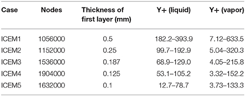
Table 1. Grids information.
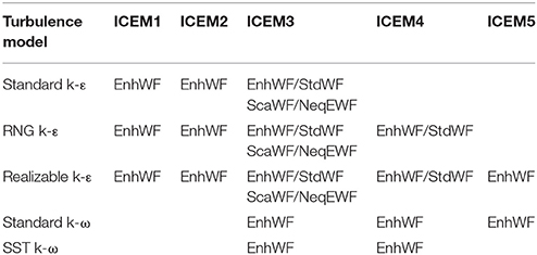
Table 2. Computational matrixes of grids, turbulence model and wall function.
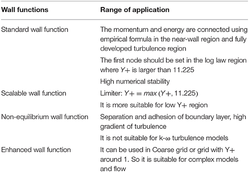
Table 3. Wall functions.
Not all the possible combinations are calculated in this paper for the numerous computational time and resource. Because of the same basic mechanism for the three k-ε models, the results of each can be used to the others. So the simulation of ICEM1 to ICEM5 on Realizable k-ε models and enhanced wall function are calculated to investigate the effect of different grids. This work is also done for the standard k-ω models on ICEM3~ICEM5. The effect of turbulence models are compared based on ICEM3 and ICEM4. We believe the conclusion can be extended to the other grids. For the wall function part, different wall functions can only be used on different k-ε models. So in the k-ω models, no wall functions are calculated except the enhanced wall function.
The effect of grid type, grids number, turbulence and wall functions are discussed below. Results are compared among the highest temperature values and dry-out location of the inner surface of the pipe. The temperature distribution is the key safe-relative parameter in the CHF experiment and should be paid more attention to discuss.
As has been validated, the grid type has limit influence on the temperature distribution in single phase flow. But for two phase flow, a little difference is found among three grid types. The grid types are shown in Figure 2, and the numbers of nodes are 1344000, 1298500, and 1228500 separately. Figure 3 shows the temperature distribution of the inner surface of the pipe. Results show all the three grids have the same dry-out position while the highest temperature values are different. More detail information can be found in Figure 4 which is the radial temperature distribution at 4.5 m. The distribution of Hexaprism grid shows a little decentered phenomenon which is not in accordance with theory. Furthermore, the distribution in Triprism grid shows a zigzag in the center of the channel. Though this phenomenon can be avoided through refining the grid, it will cost more computing resource and time. So to predict the dry-out position and highest temperature value accurately, O type or axis-symmetric grid should be chosen for the calculation.
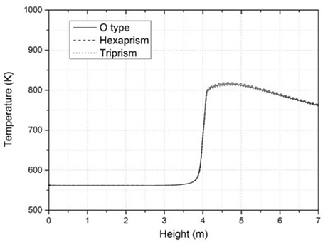
Figure 3. Temperature distribution of the inner surface of the pipe.
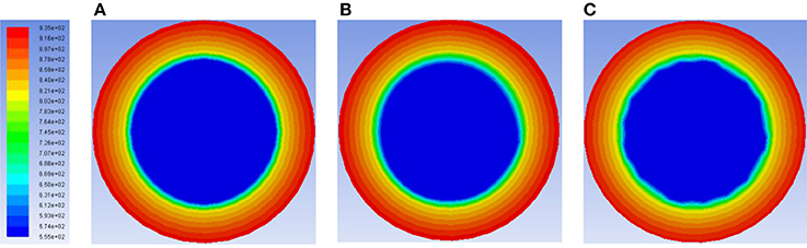
Figure 4. Radius distribution of temperature at the 4.5 m height. (A) O type grid. (B) Hexaprism grid. (C) Triprism grid.
Grid independent calculation is always an important requirement in the numerical simulation. It is necessary to estimate the quality of gird through the calculations of different grids' level. However, it is not easy to gain fully grid-independent results for all the simulation, especially for two phase flow. But It has been tested that all the k-ε models and k-ω models with enhanced wall function can be used for a large scale of Y+ values from one to hundreds in single phase flow. Zhang et al. (2015) had also investigated the effect of grids and Y+ values in the subcooled boiling flow. It is concluded that results of k-ε models match well with experiment data when near-wall grid Y+ is larger than 11.25 and enhanced wall function cannot cope with the grids with wall adjacent grid Y+ near to 1. However, results of CHF calculation show a different conclusion which has a more strict limitation for Y+ value.
Figure 5 show the comparison of the surface temperature under different grids on standard k-ε model and enhanced wall function. Results show little difference is detected among different grids except the highest temperature. The simulation results show a good match with experimental data. The dry-out positions of simulation results and experimental data are also in accord with each other. What's more, the difference of highest temperature decreased along with the refinement of the grids. So it may have the trend to gain grid-independent results.
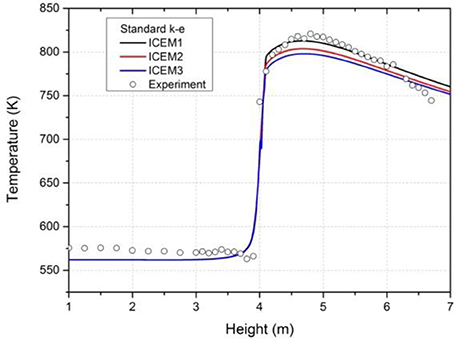
Figure 5. Surface temperatures under different grids on standard k-ε model and enhanced wall function.
The surface temperature results including ICEM4 are shown in Figure 6, and it is calculated based on RNG k-ε model and enhanced wall function. As we can see from Figure 6, the dry-out position of ICEM4 falls behind that of the other three grids. The highest value of surface temperature of ICEM4 is also much lower than that of the other three grids and the experimental data. So the results start to be worse along with the refinement of grid and the decrease of the Y+ value.
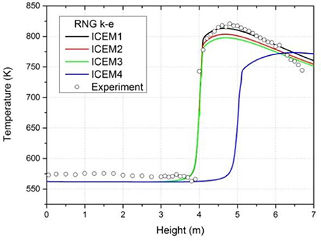
Figure 6. Surface temperatures under different grids on RNG k-ε model and enhanced wall function.
For a further validation, the comparison results including the ICEM5 are shown in Figure 7 which is calculated based on Realizable k-ε model and enhanced wall function. The temperature distribution of ICEM 4 shows same trend as that in Figure 6. The dry-out position is found behind the others and the highest temperature value is lowest. We can also see from Figure 6 that when compared with good performance of the other grids, the temperature distribution of ICEM5 shows a large fluctuation in 0.7-2.5m. What's more, the highest temperature is lower than the other four. After applying ICEM3, ICEM4 and ICEM5 with Standard k-ω model, we also found same phenomena in the same position. The results are shown in Figure 8. The Y+ value of ICEM 5 is shown in Figure 9. After comparing this two figure, we found that this unreasonable phenomena mainly appear near the wall when the Y+ value is lower than 50. The reason is that the transient behavior of bubbles has a great influence on the space averaged property when the near wall cells are too small.
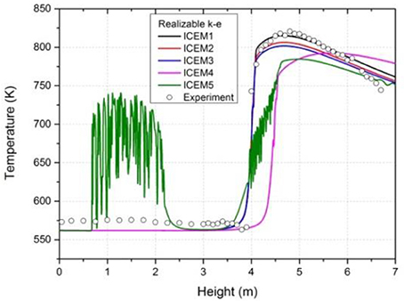
Figure 7. Surface temperatures under different grids on Realizable k-ε model and enhanced wall function.
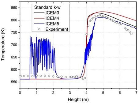
Figure 8. Surface temperatures under different grids on Standard k-ω model.
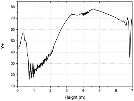
Figure 9. Y+ value of ICEM5 on Realizable k-ε model and enhanced wall function.
Different turbulence models are applied to the CHF calculation with enhanced wall function based on ICEM3 and ICEM4. The results are shown in Figures 10, 11. Some of the results show good agreement with experimental data while the others not.
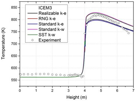
Figure 10. Surface temperatures under different turbulence models on ICEM3.
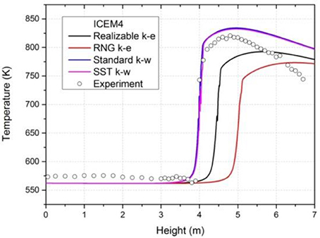
Figure 11. Surface temperatures under different turbulence models on ICEM4.
Figure 10 shows the inner surface temperature distribution of the pipe which is calculated under different turbulence models on ICEM3. Little difference is detected between Standard k-ω model and SST k-ω model. Only the highest value of temperature shows a difference about 2-5K which can be ignored. The results of Standard k-ε model and RNG k-ε model are nearly the same while both of these two are slightly lower than the results of Realizable k-ε model. The highest value of temperature of k-ω models is 30K higher than that of k-ε models which is a considerable difference. However, when compared with experimental data, all the simulation results are acceptable. The predicted dry-out position and temperature distribution are in accord with experimental data.
When ICEM4 is employed to the CHF calculation, large differences are found among the different turbulence models. The results are shown in Figure 11. The two k-ω models still show similar results in dry-out position and temperature distribution. Furthermore, these two results are also in agreement with experimental data except the post-dryout position. For k-ε models, the dry-out positions are predicted behind the experimental data and the highest temperatures are also lower than the measurement. It is worth to say that all the above calculations are under enhanced wall function. The effect of wall functions will be discussed in next section.
Heat transfer and flow characters in near wall regions are important to the calculation of temperature and velocity in two-phase flow. The wall functions and wall boiling model are also influenced by each other. Because the wall functions use different empirical correlations to solve the equations in viscous sublayer and buffer layer, different wall functions will have different performance. In FLUENT, k-ω models are low Reynolds models and set to be used with wall functions unless the grid Y+ doesn't meet the requirements of the low Reynolds number modeling. If the requirements are met, then FLUENT doesn't apply wall function but resolves the near wall region. So there is no need to discuss the effect of different wall functions when use k-ω models.
Based on ICEM3, the CHF calculation results of k-ε models under different wall functions are shown in Figure 12 separately. All these three pictures show same trend for different wall functions. The temperature of non-equilibrium wall functions is 20K higher than that of the others while the enhanced wall function has the lowest temperature. The temperature distributions of standard wall function and scalable wall function are the same. This is determined by the correlation of scalable wall function.
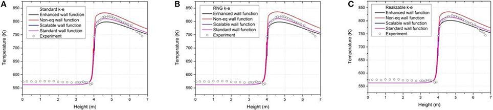
Figure 12. Surface temperatures under different wall functions on (A) Standard k-ε model, (B) RNG k-ε model, (C) Realizable k-ε model.
The purpose of scalable wall functions is to force the usage of the log law in conjunction with the standard wall functions approach. This is achieved by adding a limiter in the Y+ calculations Y + is calculated by
So when the Y+ is larger than 11.25, Y+ is the same with original value, and then the scalable wall function is the same as standard wall function. Otherwise, Y+ is equal to 11.25 which bring different results. For the cases in this paper, all the Y+ values are larger than 11.25, so there is no difference for the results between these two wall functions. When compared with experimental data, the standard wall function and scalable wall function show the best performance while results of the other two are also acceptable.
Based on ICEM4, the comparison is only investigated between standard wall function and enhanced wall function on two k-ε models. The results are shown in Figure 13. As mentioned above, the predicted dry-out positions of enhanced wall function are behind the measurement when ICEM4 is employed to the simulation. Among these four cases, only Realizable k-ε model with standard wall function can give an accurate dry-out position and acceptable temperature distribution.
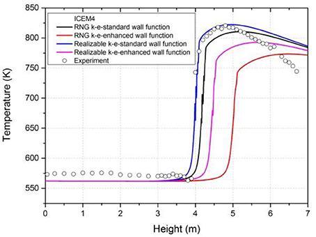
Figure 13. Surface temperatures under different wall functions on ICEM4.
CHF phenomenon in a vertical pipe is investigated by use of CFD simulation. Simulations are calculated among different grids type, grids number, different turbulence models and wall functions to detect the effect of these parameters. Several conclusions are obtained after comparing the simulation results and experimental data. The conclusion about the effect of grid and turbulence models can help someone reduce their workload on mesh validation and set up solve algorithm quickly.
(1) type or axis-symmetric grid is recommended for the CFD simulation of vertical pipe or the other geometries.
(2) Grids with Y+ larger than 70 are recommended for the CHF simulation while Grids with Y+ lower than 50 should be avoided for the simulation of CHF phenomenon in the vertical pipe.
(3) The temperature distributions of k-ω models are 20K higher than that of k-ε models in all the cases. But they are all acceptable when comparing with experimental data.
(4) The predicted dry-out position of enhanced wall function is always behind that of the others if used with a fine grid. To predict the dry-out position accurately in a refine grid, Realizable k-ε model with standard wall function is recommended.
XD is the main author of the paper, he finished the research and write. ZZ is the supervisor and give the guide for the other authors. DL is the co-author who works for the comparison of the experiment and simulation. ZT is the associated supervisor and give the reference too. GC works with the other authors for the discussion part.
The authors declare that the research was conducted in the absence of any commercial or financial relationships that could be construed as a potential conflict of interest.
This work is supported by the Research on Key Technology of Numerical Reactor Engineering (J121217001), and the authors also appreciate deeply the suggestions from Dr. Tenglong Cong.
Antal, S. P., Lahey, R. T., and Flaherty, J. E. (1991). Analysis of phase distribution in fully developed laminar bubbly two-phase flow. Int. J. Multiphase Flow 17, 635–652. doi: 10.1016/0301-9322(91)90029-3
Becker, K. M. (1983). An Experimental Investigation of Post Dryout Heat Transfer. Department of Nuclear Reactor Engineering, Royal Institute of Technology, KTH-NEL-33.
Bertodano, L. D. (1991). Turbulent Bubbly Flow in a Triangular Duct. Ph.D. Thesis. Rensselaer Polytechnic Institute, Troy, New York, NY.
Chen, G. L., Zhang, Z. J., Tian, Z. F., Dong, X. M., and Ju, H. R. (2017a). Design of a CFD scheme using multiple RANS models for PWR. Ann. Nucl. Energy. 102, 349–358. doi: 10.1016/j.anucene.2016.12.030
Chen, G. L., Zhang, Z. J., Tian, Z. F., Li, L., and Dong, X. M. (2017b). Challenge analysis and schemes design for the CFD simulation of PWR. Sci. Technol. Nucl. Installations. 2017:5695809. doi: 10.1155/2017/5695809
Cole, R. (1960). A photographic study of pool boiling in the region of the critical heat flux. AIChE J. 6, 533–542. doi: 10.1002/aic.690060405
Del Valle, V. H., and Kenning, D. B. R. (1985). Subcooled flow boiling at high heat flux. Int. J. Heat Mass Transf. 28, 1907–1920. doi: 10.1016/0017-9310(85)90213-3
Drew, D. A., and Lahey, R. T. (1993). In Particulate Two-Phase Flow. Boston, MA: Butterworth-Heinemann.
Hua, S. Y., Huang, R. H., and Zhou, P. (2015). Numerical investigation of two-phase flow characteristics of subcooled boiling in IC engine cooling passages using a new 3d two-fluid model. Appl. Therm. Eng. 90, 648–663. doi: 10.1016/j.applthermaleng.2015.07.037
Ishii, M. (1979). “Two-fluid model for two-phase flow,” in Proceedings of the 2nd International Workshop on Two-phase Flow Fundamentals. Troy, NY: RPI.
Kim, S. E., Choudhury, D., and Patel, B. (1999). “Computations of complex turbulent flows using the commercial code fluent,” in Modeling Complex Turbulent Flows, eds M. Salas, J. Hefner, and I. Sakell (Dordrecht: Springer), 259–276.
Krepper, E., Koncar, B., and Egorov, Y. (2007). CFD modelling of subcooled boiling—concept, validation and application to fuel assembly design. Nucl. Eng. Des. 237, 716–731. doi: 10.1016/j.nucengdes.2006.10.023
Krepper, E., and Rzehak, R. (2011). CFD for subcooled flow boiling: simulation of debora experiments. Nucl. Eng. Des. 241, 3851–3866. doi: 10.1016/j.nucengdes.2011.07.003
Krepper, E., Rzehak, R., Lifante, C., and Frank, T. (2013). CFD for subcooled flow boiling: coupling wall boiling and population balance models. Nucl. Eng. Des. 255, 330–346. doi: 10.1016/j.nucengdes.2012.11.010
Kurul, N., and Podowski, M. Z. (1991). “On the modeling of multidimensional effects in boiling channels,” in Proceedings of the 27th National Heat Transfer Conference (Minneapolis, MN).
Launder, B. E., and Spalding, D. B. (1972). Lectures in Mathematical Models of Turbulence. London: Academic Press.
Launder, B. E., and Spalding, D. B. (1974). The numerical computation of turbulent flows. Comput. Methods Appl. Mech. Eng. 3, 269–289. doi: 10.1016/0045-7825(74)90029-2
Lavieville, J., Quemerais, E., Mimouni, S., Boucker, M., and Mechitoua, N. (2005). NEPTUNE CFD V1.0 Theory Manual. EDF.
Lemmert, M., and Chawla, L. M. (1977). “Influence of flow velocity on surface boiling heat transfer coefficient,” in Heat Transfer Boiling, eds E. Hahne and U. Grigull (New York, NY: Academic Press and Hemisphere).
Menter, F. R. (1994). Two-equation eddy-viscosity turbulence models for engineering applications. AIAA J. 32, 1598–1605. doi: 10.2514/3.12149
Mimouni, S., Baudry, C., Guingo, M., Lavieville, J., Merigoux, N., and Mechitoua, N. (2016). Computational multi-fluid dynamics predictions of critical heat flux in boiling flow. Nucl. Eng. Des. 299, 28–36. doi: 10.1016/j.nucengdes.2015.07.017
Moraga, F. J., Bonetto, R. T., and Lahey, R. T. (1999). Lateral forces on spheres in turbulent uniform shear flow. Int. J. Multiphase Flow 25, 1321–1372. doi: 10.1016/S0301-9322(99)00045-2
Ranz, W. E., and Marshall, W. R. (1952). Evaporation from drops, chemical engineering. Progress 48, 141–146.
Shih, T. H., Liou, W. W., Shabbir, A., Yang, Z., and Zhu, J. (1995). A new k-ε Eddy-viscosity model for high reynolds number turbulent flows-model development and validation. Comput. Fluids 24, 227–238. doi: 10.1016/0045-7930(94)00032-T
Shin, B. S., and Chang, S. H. (2009). CHF experiment and CFD analysis in a 2 × 3 rod bundle with mixing vane. Nucl. Eng. Des. 239, 899–912. doi: 10.1016/j.nucengdes.2009.01.011
Shirvan, K. (2016). Numerical investigation of the boiling crisis for helical cruciform-shaped rods at high pressures. Int. J. Multiphase Flow 83, 51–61. doi: 10.1016/j.ijmultiphaseflow.2016.03.014
Tentner, A., Lo, S., and Kozlov, V. (2006). “Advances in computational fluid dynamics modeling of two-phase flow in a boiling water reactor fuel assembly,” in International Conference on Nuclear Engineering (Miami, FL).
Thakrar, R., Murallidharan, J., and Walker, S. P. (2016). CFD Investigation of nucleate boiling in non-circular geometries at high pressure. Nucl. Eng. Des. 312, 410–421. doi: 10.1016/j.nucengdes.2016.08.020
Tolubinski, V. I., and Kostanchuk, D. M. (1970). “Vapor bubbles growth rate and heat transfer intensity at subcooled water boiling,” in Proceedings of the 4th International Heat Transfer Conference (Paris).
Yakhot, V., and Orszag, S. A. (1986). Renormalization group analysis of turbulence i basic theory. J. Sci. Comput. 1, 1–51. doi: 10.1007/BF01061452
Keywords: numerical investigation, Critical heat flux, turbulence models, wall functions, grids distribution
Citation: Dong X, Zhang Z, Liu D, Tian Z and Chen G (2018) Numerical Investigation of the Effect of Grids and Turbulence Models on Critical Heat Flux in a Vertical Pipe. Front. Energy Res. 6:58. doi: 10.3389/fenrg.2018.00058
Received: 20 April 2018; Accepted: 05 June 2018;
Published: 03 July 2018.
Edited by:
Kaiyi Shi, Liupanshui Normal University, ChinaReviewed by:
Claudio Tenreiro, University of Talca, ChileCopyright © 2018 Dong, Zhang, Liu, Tian and Chen. This is an open-access article distributed under the terms of the Creative Commons Attribution License (CC BY). The use, distribution or reproduction in other forums is permitted, provided the original author(s) and the copyright owner(s) are credited and that the original publication in this journal is cited, in accordance with accepted academic practice. No use, distribution or reproduction is permitted which does not comply with these terms.
*Correspondence: Zhijian Zhang, emhhbmd6aGlqaWFuX2hldUBocmJldS5lZHUuY24=
Disclaimer: All claims expressed in this article are solely those of the authors and do not necessarily represent those of their affiliated organizations, or those of the publisher, the editors and the reviewers. Any product that may be evaluated in this article or claim that may be made by its manufacturer is not guaranteed or endorsed by the publisher.
Research integrity at Frontiers
Learn more about the work of our research integrity team to safeguard the quality of each article we publish.