A Hybrid Semi-implicit Method of 1D Transient Compressible Flow for Thermal-Hydraulic Analysis of (V)HTR Gas Turbine Systems

Transient thermal-hydraulic analysis of (very) high temperature gas-cooled reactors gas turbine systems (HTRGTSs) needs system transient analysis codes. However, compared with the mature system transient thermal-hydraulic codes of pressurized water reactors (PWRs), the system analysis codes of HTRGTSs have not been so fully developed. In this paper, a new hybrid semi-implicit (HSI) method is proposed based on the semi-implicit method and nearly-implicit method. In the HIS method, a new calculation strategy is devised: the convective term is treated explicitly to solve pressure and velocity, while density and temperature are solved in an implicit manner to get a convergent, stable, and accurate solution in multiple transient scenarios. The HSI method was further validated via the shock-tube benchmark problem and verified via FLUENT simulations. In FLUENT simulations, outlet pressure transient, inlet mass flow transient and inlet temperature transient were studied. It was found that the HSI method is capable of capturing both the fast and slow compressible flow transients with good convergence and stability. Furthermore, an adaptive time step scheme is proposed for faster calculations, considering the maximum relative density difference and Courant–Friedrichs–Lewy condition.

Introduction

High temperature gas-cooled reactors gas turbine system (HTRGTS) is inherently safe and highly efficient with a reactor outlet temperature of 700~1,000°C. HTRGTS uses a Brayton cycle, which includes a reactor, one or two compressors, turbine, recuperator, precooler, and intercooler. The working medium is usually helium in the HTRGTS because of its chemical inertia. The helium in the Brayton cycle is compressed to very high pressure (e.g., 7 MPa) in compressors and furtherly heated through the reactor, and then expands to very low pressure (e.g., 2.7 MPa) to generate kinetic energy in the turbine.

There is a very big pressure difference in different parts of HTRGTS during normal operation, ranging from 2.7 MPa to 7.0 MPa, and moreover the pressure changes quickly during accidents. Since helium is compressible, a compressible transient system analysis code is very important and necessary to the accident analysis of HTRGTS, and it has been studied since 1970s. However, because the HTRGTS is not so widely and commercially used as the pressurized water reactors (PWRs), transient system analysis codes for HTRGTS are not so well developed as those of PWRs. Different from PWRs, HTRGTS uses helium as its working fluid, whose density strongly couples with pressure and temperature. Consequently, compressibility should be considered in the transient calculations of HTRGTS for more accurate solutions, especially when significant changes of pressure and temperature are involved.

To date, the developed system analysis codes related to HTRGTS include GTSim for MGR-GT and GTMHR-300 program in Japan, FLOWNEX for PBMR program in South Africa, and PLAYGAS and CATHARE2 in Europe. In GTSim(Yan, 1990), a one-dimensional compressible flow model was used to simulate the transient conditions. The numerical method used in GTSim is a non-iterative method that provides the strong coupling between energy and continuity equations, and the strong coupling between energy and momentum equations. However, in this method the coupling between continuity and momentum equations is not very strong. As a result, this method is not very good in solving pressure transients, where continuity and momentum equations are strongly coupled.

FLOWNEX (Greyvenstein, 2002; Rousseau et al., 2006; van Ravenswaay et al., 2006) uses an implicit pressure correction method, which is very similar to the- SIMPLE method (Patankar, 1980; Tao, 2001). This method strongly couples the continuity and momentum equations, but it does not couple the energy equation. The energy equation is solved independently after continuity and momentum equations are solved. Besides, as a system solver for one dimensional transient compressible flow, this method has two weaknesses: (1) it is an iterative method that may require many iteration steps for each time step, especially in solving the transient compressible flow, such as pressure transients; and (2) it requires the setting of a pressure relaxation factor, which is an empirical figure depending on transient conditions and user experiences, and thus greatly affects computational time. These two weaknesses limit its use in the system analysis codes of HTRGTS.

The CATHARE series codes (Widlund et al., 2005; Saez et al., 2006; Bentivoglio et al., 2008) use a fully-implicit time integration scheme for zero-dimensional and one-dimensional modules. This method represents a relatively larger computational effort, which might be compensated by the increased numerical stability and the possibility to choose greater time steps for slow and long transients (Bestion, 2008). However, in solving the transient compressible flow where there is a very strong coupling of pressure, temperature, and density, the fully implicit integration scheme requires too many iteration steps for a converged solution, especially in fast pressure transients.

Therefore, it is meaningful to devise a non-iterative method that requires less computational time in solving fast pressure transients, and allows greater time step in solving slow temperature transients. There is a potential of using the methods in other fully developed codes of PWRs, such as the non-iterative semi-implicit and nearly-implicit methods (Division, 2001), for the transient solvers of HTRGTS.

The structure of this paper is as follows. Section Analysis of Semi-Implicit and Nearly-Implicit Methods in Compressible Flow analyzes the performances of the semi-implicit and nearly-implicit methods in solving compressible flow transients. Section A New Hybrid Semi-Implicit Method Proposes an Improved Non-Iterative Semi-Implicit Method, that is, Hybrid Semi-Implicit (HSI) method, based on the discussion of the semi-implicit and nearly-implicit methods. Section Verification of Hybrid Semi-Implicit presents the verification of the HSI method via shock tube benchmark problem and the comparisons of the HSI method with FLUENT simulations, in which an outlet pressure transient, an inlet mass flow transient and an inlet temperature transient are studied. Section Adaptive Time Step proposes an adaptive time step scheme for the HIS method for faster calculation speed. Section Conclusions presents the final conclusions.

Analysis of Semi-implicit and Nearly-implicit Methods in Compressible Flow

Solution Strategies of Semi-implicit and Nearly-Implicit Methods

One Dimensional Conservative Equations

In a pipe with a constant cross section area, the one-dimensional continuity, momentum and energy equations are, respectively,

$\begin{array}{cc}\frac{\partial \rho }{\partial \tau }+\frac{\partial \rho u}{\partial x}=0& \left(1\right)\end{array}$

$\begin{array}{cc}\rho \frac{\partial u}{\partial \tau }+\frac{1}{2}\rho c_m\frac{\partial u^2}{\partial x}=-\frac{\partial p}{\partial x}-f_w\rho u& \left(2\right)\end{array}$

$\begin{array}{cc}{c}_v\frac{\partial \rho T}{\partial \tau }+c_v\frac{\partial \rho uT}{\partial x}=-p\frac{\partial u}{\partial x}+\frac{h{D}_e}{A_c}(T_w-T)& \left(3\right)\end{array}$

In the discritization process of the semi-implicit and nearly-implicit methods, the control volume is shown in Figure 1, in which [x_i, x_i+1] is control volume of density, pressure and temperature, and [x_K, x_L] is control volume of velocity. A first order upwind scheme is adopted for cell face density and temperature, and a central difference scheme is used for cell center velocity.

FIGURE 1

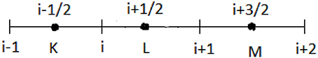
Figure 1. Discritized nodes.

Semi-implicit Method

Discretize continuity and energy Equations (1) and (3), respectively, yields

$\begin{array}{cc}{\tilde{\rho }}_L^{n+1}-{\rho }_L^n+({\dot{\rho }}_{i+1}^n{u}_{i+1}^{n+1}-{\dot{\rho }}_i^n{u}_i^{n+1})\frac{\Delta \tau }{\Delta x}=0& \left(4\right)\end{array}$

$\begin{array}{cc}\begin{array}{l}\left({\tilde{\rho }}_L^{n+1}-{\rho }_L^n\right)T_L^n+{\rho }_L^n\left({\tilde{T}}_L^{n+1}-T_L^n\right)-{\left[\frac{h{D}_e}{c_v{A}_c}(T_w-T)\right]}_L^n\\ \Delta \tau =-\left[\left({\dot{\rho }}_{i+1}^n{\dot{T}}_{i+1}^n+\frac{P_L^n}{c_v}\right)u_{i+1}^{n+1}-\left({\dot{\rho }}_i^n{\dot{T}}_i^n+\frac{P_L^n}{c_v}\right)u_i^{n+1}\right]\frac{\Delta \tau }{\Delta x}\end{array}& \left(5\right)\end{array}$

According to Taylor expansion, we get the expression of density ρⁿ⁺¹ in term of Pⁿ⁺¹and Tⁿ⁺¹:

$\begin{array}{cc}{\tilde{\rho }}_L^{n+1}={\rho }_L^n+{\left(\frac{\partial \rho }{\partial P}\right)}_L^n\left(P_L^{n+1}-P_L^n\right)+{\left(\frac{\partial \rho }{\partial T}\right)}_L^n\left({\tilde{T}}_L^{n+1}-T_L^n\right)& \left(6\right)\end{array}$

Substitute Equation (6) into energy Equation (5) and eliminate the density term ρⁿ⁺¹ yields expression of the next-time step temperature Tⁿ⁺¹ in term of Pⁿ⁺¹ and uⁿ⁺¹:

$\begin{array}{cc}\begin{array}{l}{\tilde{T}}_L^{n+1}=T_L^n-{\left(\frac{\partial T}{\partial \rho }\right)}_L^n{\left(\frac{\partial \rho }{\partial P}\right)}_L^n\left(P_L^{n+1}-P_L^n\right)\\ -{\left(\frac{\partial T}{\partial \rho }\right)}_L^n\left({\dot{\rho }}_{i+1}^n{u}_{i+1}^{n+1}-{\dot{\rho }}_i^n{u}_i^{n+1}\right)\frac{\Delta \tau }{\Delta x}\end{array}& \left(7\right)\end{array}$

Combining Equations (5)~(7) to eliminate the terms of ρⁿ⁺¹ and Tⁿ⁺¹ yields expression of the next time step pressure Pⁿ⁺¹ in term of uⁿ⁺¹:

$\begin{array}{cc}{P}_L^{n+1}=P_L^n+l_L^n{u}_i^{n+1}-r_L^n{u}_{i+1}^{n+1}-E_L^n\Delta \tau ·{\left(\frac{\partial \rho }{\partial T}\right)}_L^n/{\left(\frac{\partial \rho }{\partial P}\right)}_L^n& \left(8\right)\end{array}$

Then, discretize the momentum equation in Equation (2)

$\begin{array}{cc}\begin{array}{l}{\rho }_i^n\left(u_i^{n+1}-u_i^n\right)+\frac{1}{2}{\dot{\rho }}_i^n{c}_{m,i}[{\left(u_L^n\right)}^2-{\left(u_K^n\right)}^2-u_L^n(u_{i+1}^n-u_i^n)\\ +u_K^n(u_i^n-u_{i-1}^n)]\frac{\Delta \tau }{\Delta x}=-\left(P_L^{n+1}-P_K^{n+1}\right)\frac{\Delta \tau }{\Delta x}-f_{w,i}^n{\rho }_i^n{u}_i^{n+1}\Delta \tau \end{array}& \left(9\right)\end{array}$

The expression of the next-time step velocity uⁿ⁺¹ in term of Pⁿ⁺¹can be derived:

$\begin{array}{cc}{u}_i^{n+1}=c_i^n\left(P_K^{n+1}-P_L^{n+1}\right)+d_i^n& \left(10\right)\end{array}$

It should be noted that the convection term in the momentum equation is treated explicitly in the semi-implicit method. The calculation strategy of the semi-implicit method is as follows:

Substitute Equation (10) into (8) to eliminate uⁿ⁺¹ yields the expression of Pⁿ⁺¹:

$\begin{array}{cc}\begin{array}{l}-c_i^n{l}_L^n{P}_K^{n+1}+(1+c_i^n{l}_L^n+c_{i+1}^n{r}_L^n)P_L^{n+1}-c_{i+1}^n{r}_L^n{P}_M^{n+1}\\ =P_L^n+l_L^n{d}_i^n-r_L^n{d}_{i+1}^n+{\rho }_L^{n}R{E}_L^n\Delta \tau \end{array}& \left(11\right)\end{array}$

Then substitute Pⁿ⁺¹into Equation (10) yields uⁿ⁺¹.

Then substitute Pⁿ⁺¹and uⁿ⁺¹ into Equation (7) yields Tⁿ⁺¹.

Then substitute Pⁿ⁺¹and Tⁿ⁺¹ into Equation (6) yields density ρ₁.

Finally, substitute Pⁿ⁺¹and Tⁿ⁺¹ into state equation yields another density ρ₂, if the difference between ρ₁ and ρ₂ is small enough, then a converged solution is obtained.

Nearly-implicit Method

In the nearly-implicit method, the continuity and energy equations are treated and the relationship between pressure and velocity is deduced. The convective term in the momentum equation is treated implicitly, as shown in Equation (12):

$\begin{array}{cc}\begin{array}{l}{\rho }_i^n\left(u_i^{n+1}-u_i^n\right)+\frac{1}{2}{\dot{\rho }}_i^n{c}_{m,i}\frac{\Delta \tau }{\Delta x}[{\left(u_L^n\right)}^2+2u_L^n\\ \left(u_L^{n+1}-u_L^n\right)-{\left(u_K^n\right)}^2-2u_K^n\left(u_K^{n+1}-u_K^n\right)]\\ -\frac{1}{2}{c}_{m,i}{\dot{\rho }}_i^n\left[u_L^n(u_{i+1}^n-u_i^n)-u_K^n(u_i^n-u_{i-1}^n)\right]\\ \frac{\Delta \tau }{\Delta x}=-\left(P_L^{n+1}-P_K^{n+1}\right)\frac{\Delta \tau }{\Delta x}-f_{w,i}^n{\rho }_i^n{u}_i^{n+1}\Delta \tau \end{array}& \left(12\right)\end{array}$

The relationship between velocity uⁿ⁺¹and pressure Pⁿ⁺¹ can be deduced from Equation (12):

$\begin{array}{cc}{A}_i{u}_{i-1}^{n+1}+B_i{u}_i^{n+1}+C_i{u}_{i+1}^{n+1}+D_i=P_K^{n+1}-P_L^{n+1}& \left(13\right)\end{array}$

Density and temperature in the nearly-implicit method are solved implicitly in continuity Equation (14) and energy Equation (15), respectively.

$\begin{array}{cc}{\tilde{\rho }}_L^{n+1}-{\rho }_L^n+({\dot{\rho }}_{i+1}^{n+1}{u}_{i+1}^{n+1}-{\dot{\rho }}_i^{n+1}{u}_i^{n+1})\frac{\Delta \tau }{\Delta x}=0& (14)\end{array}$

$\begin{array}{cc}\begin{array}{l}\left[\left({\tilde{\rho }}_L^{n+1}-{\rho }_L^n\right)T_L^n+{\rho }_L^n\left({\tilde{T}}_L^{n+1}-T_L^n\right)\right]\frac{\Delta x}{\Delta \tau }-{\left[\frac{h{D}_e}{c_v{A}_c}(T_w-T)\right]}_L^n\\ =\left({\dot{\rho }}_i^{n+1}{\dot{T}}_i^{n+1}+\frac{P_L^{n+1}}{c_v}\right)u_i^{n+1}-\left({\dot{\rho }}_{i+1}^{n+1}{\dot{T}}_{i+1}^{n+1}+\frac{P_L^{n+1}}{c_v}\right)u_{i+1}^{n+1}\end{array}& (15)\end{array}$

The calculation strategy of nearly-implicit method is in the following steps:

1) Substitute the expression of Pⁿ⁺¹ in Equation (8) into Equation (13), uⁿ⁺¹ can be solved first;

2) Then substitute uⁿ⁺¹ into Equation (8), Pⁿ⁺¹ can be solved;

3) Then substitute uⁿ⁺¹ into continuity Equation (14) and update the velocity term, density ρ₁ can be solved implicitly;

4) Then substitute uⁿ⁺¹ Pⁿ⁺¹ and ρ₁ into energy equation (15) and update the velocity, pressure and density terms, temperature can be solved implicitly;

5) Finally, substitute Pⁿ⁺¹ and Tⁿ⁺¹ into state equation, another density ρ₂ can be solved. If the difference between ρ₁ and ρ₂ is small enough, a convergent solution is obtained.

In step (3) and step (4), density and temperature are solved in the following form:

$\begin{array}{cc}{a}_{p,i}{\varphi }_L^{n+1}=a_{w,i}{\varphi }_K^{n+1}+a_{e,i}{\varphi }_M^{n+1}+b_i& \left(16\right)\end{array}$

ϕⁿ⁺¹ mean density ρⁿ⁺¹ in continuity equation and temperature Tⁿ⁺¹ in energy equation.

Performances of the Semi-Implicit and Nearly-Implicit Methods

Two FORTRAN codes were developed based on the semi-implicit and nearly-implicit methods in order to analyze their performances in solving transient compressible flow. Pressure transient involves the strong coupling of pressure, density, velocity, and temperature, and it is used to testify the performances of the two methods. The transient condition is a step decrease of outlet pressure of a pipe from 2.7 MPa to 2.6 MPa. Other parameters, such as boundary conditions, time step, and space step, are shown in Table 1. The calculated pressure and temperature responses by the two methods are shown in Figures 2, 3, respectively.

TABLE 1

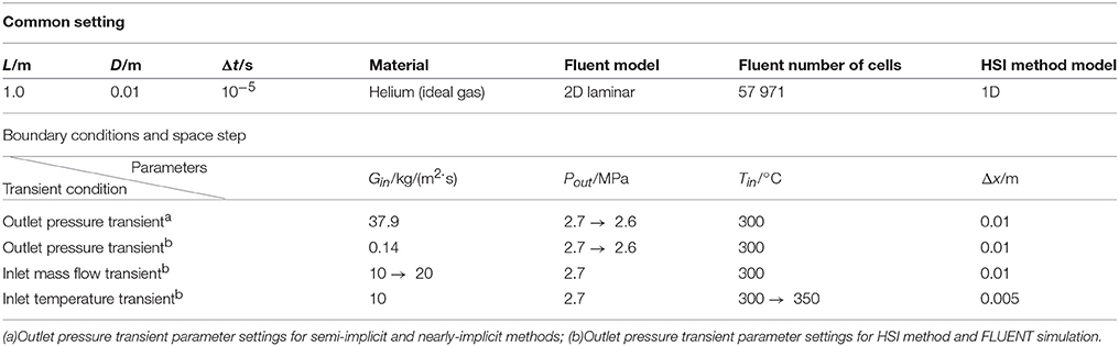
Table 1. Parameter settings.

FIGURE 2

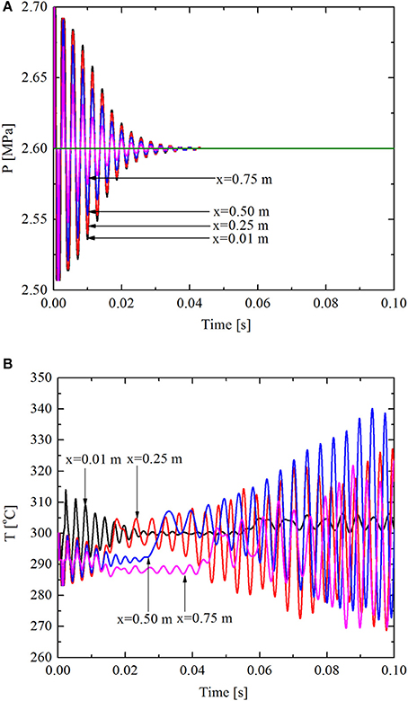
Figure 2. Responses of the semi-implicit method under outlet pressure transient. (A) Pressure responses. (B) Temperature responses.

FIGURE 3

Figure 3. Responses of the nearly-implicit method under outlet pressure transient. (A) Pressure responses. (B) Temperature responses.

It can be seen from Figure 2A that the semi-implicit method is capable of capturing the fast pressure responses with little numerical diffusion. However, it has poor stability in capturing the slow temperature responses, as seen in Figure 2B that temperature diverged at 0.02 ~ 0.04 s. It can be seen from Figure 3B that the nearly-implicit method has good stability in capturing the slow temperature responses. However, it cannot capture the fast pressure responses very accurately, as seen in Figure 3A that the pressure oscillations are suppressed and vanish very quickly.

One possible reason for the great numerical diffusion of the nearly-implicit method is that the time step Δτ = 10⁻⁵ s is too large to capture the fast pressure responses accurately. The variation of time step from 10⁻⁶ s to 10⁻⁸ s was studied, and some of the results are shown in Figure 4. It was found that if time step Δτ ≤ 10⁻⁷ s, the numerical diffusion of pressure can be very small. However, there are two weaknesses: (1) spurious oscillations exist at the pressure step change points; and (2) the time step is too small, which means a great computational effort.

FIGURE 4

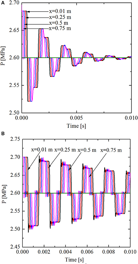
Figure 4. Pressure responses of the nearly-implicit method under different time steps. (A) Δt = 10⁻⁶s. (B) Δt = 10⁻⁷s.

As shown in Figures 2~4, neither the semi-implicit method nor nearly-implicit method provides a stable and accurate solution in solving transient compressible flow.

A New Hybrid Semi-implicit Method

Further Discussion of the Semi-implicit and Nearly-Implicit Methods

For the semi-implicit method, velocity is implicit while density is explicit in continuity equation. In energy equation, only velocity is implicit, the other parameters, such as density, pressure, and temperature, are all explicit. In momentum equation, the pressure and frictional terms are implicit, while the convective term is explicit. So the expressions of density, temperature, velocity, and pressure can be derived directly. In calculation, firstly, pressure, density and temperature are solved explicitly from the derived expressions, and then velocity is solved based on the solved pressure.

In the nearly-implicit method, the expression of pressure is derived from continuity and energy equations in the same way as in the semi-implicit method. Different from the semi-implicit method, the convective term in the momentum equation is treated implicitly. In calculation, velocity is solved first, then pressure is solved subsequently based on the solved velocity, and then density and temperature are solved implicitly by updating the solved pressure, velocity and density in continuity and energy equations.

There are mainly two differences between the semi-implicit and nearly-implicit methods: (1) the explicit or implicit treatment of the convective term in the momentum equation, which determines the different expressions of velocity, and (2) the explicit or implicit calculation of density and temperature. According to the two differences and the results in Figures 2–4, it is assumed that (1) in order to capture a detailed fast pressure transient response, the convective term in momentum equation should be treated explicitly, and (2) in order to get a stable solution for the slow temperature transients, coefficients in the continuity, and energy equations should be updated immediately using the previously solved parameters, such as pressure, velocity and density.

To testify this hypothesis, the convective term in momentum equation is treated implicitly as in the nearly-implicit method, and density and temperature are solved explicitly as in the semi-implicit method. If this hypothesis was correct, it is predicted that neither an accurate pressure response nor a stable temperature solution could be obtained. The results are shown in Figure 5, in which the time step is Δτ = 10⁻⁵ s. It can be seen that for the fast pressure response, the artificial diffusion is too big, while for the slow temperature response, the solution diverged. The results are the same as predicted, so the hypothesis is reasonable.

FIGURE 5

Figure 5. Responses of the hypothesized opposite treatments under outlet pressure transient. (A) Pressure responses. (B) Temperature responses.

Proposal of a New Hybrid Semi-implicit Method

According to the hypothesis discussed above, a new HSI method is proposed. In the HSI method, the convective term in momentum equation is treated explicitly, and density and temperature are solved implicitly by updating coefficients in the continuity and energy equations using the previously solved parameters. The calculation strategy of the HSI method is in the following steps:

1) First, Pⁿ⁺¹ is solved in Equation (11);

2) Then substitute Pⁿ⁺¹ into the momentum Equation (10) and solve uⁿ⁺¹;

3) Then substitute uⁿ⁺¹ into the continuity Equation (14) to update velocity term and solve density ρ₁ implicitly;

4) Then substitute ρ₁, uⁿ⁺¹ and Pⁿ⁺¹ into the energy Equation (15) to update density, velocity and pressure terms and solve Tⁿ⁺¹ implicitly.

5) Finally, substitute Pⁿ⁺¹ and Tⁿ⁺¹ into state equation, another density ρ₂ can be calculated, if the difference between ρ₁ and ρ₂ is small enough, a convergent solution is obtained.

Under the same outlet pressure transient in section Analysis of Semi-Implicit and Nearly-Implicit Methods in Compressible Flow, and using parameter settings in Table 1, the pressure and temperature responses of the HSI method are shown in Figure 6. It can be seen from Figures 6A,B that the fast transient responses caused by pressure oscillations are captured and the slow temperature responses are stable and converged. As a result, the newly proposed HSI method has the advantages of both the semi-implicit and nearly-implicit methods but none of their weaknesses.

FIGURE 6

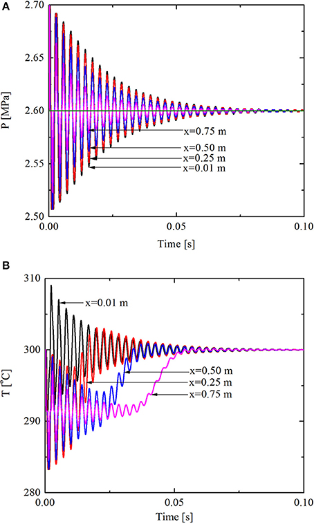
Figure 6. Responses of the hybrid semi-implicit under outlet pressure transient. (A) Pressure responses. (B) Temperature responses.

Verification of Hybrid Semi-implicit

The newly proposed HSI method has shown good performance in solving transient compressible flow. However, the accuracy of the results needs to be further verified. The HSI method was furtherly verified via the shock tube benchmark problem, and compared with FLUENT simulations.

Shock Tube Benchmark Problem

The shock tube problem is a typical Riemann problem, and has an exact solution (Toro, 2009). In the shock tube problem, a closed tube with a length of 100 m was separated into two equal parts by a membrane film, as shown in Figure 7. The left part of the tube is helium with a pressure of 2.0 MPa and a temperature of 400 K, and the right part of the tube is helium with a pressure of 1.0 MPa and a temperature of 400 K. If the film suddenly breaks in the center, the helium in two parts mixes together, and shock wave, rarefaction wave, and discontinuity wave are produced in this process.

FIGURE 7

Figure 7. The shock tube problem model.

There is no exact closed-form solution to the Riemann problem for the Euler equations of shock-tube problem. However, it is possible to devise iterative schemes whereby the solution can be computed numerically to high accuracy. The space step is set as 0.05 m in both the iterative scheme and the HSI method. Comparison of the exact solution with that of the HSI method is shown in Figure 8. Three time steps of 10⁻⁴ s, 10⁻⁵ s, and 10⁻⁶ s are calculated using the HSI method. It was found that when Δτ = 10⁻⁴ s the solution is divergent, and when Δτ = 10⁻⁵ s and Δτ = 10⁻⁶ s, the results of the HSI method are almost identical, as seen in Figure 8. So the time step is set as 10⁻⁵ s in this case to get a convergent solution with shorter computational time in the following discussion.

FIGURE 8

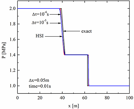
Figure 8. Comparisons between the HSI method and the exact solution.

It can be seen from Figure 8 that the HSI method can capture the pressure transient with good accuracy. The slope of each wave nearly equals to the exact solution and there are no spurious oscillations at pressure step change points.

Comparisons With Fluent Simulations

In this section, the HSI method was compared with FLUENT simulations in which a two-dimensional laminar flow model was adopted. In the FLUENT simulations, constant outlet pressure, inlet mass flow, and inlet temperature were adopted for the boundary conditions of compressible flow. In order to test the performances of the HSI method under different transient scenarios, three typical transient conditions are studied and compared with FLUENT simulations, namely an outlet pressure transient, inlet mass flow transient, and inlet temperature transient. Among the three transients, the pressure transient is a fast transient with a very short characteristic time that involves significant changes of pressure, velocity, and temperature. The mass flow transient is also a fast transient but does not involve significant changes of pressure or temperature. The temperature transient is a slow transient with a long characteristic time, and causes mild changes of pressure, velocity, and temperature.

Outlet Pressure Transient

The transient condition for outlet pressure transient is a step decrease of outlet pressure from 2.7 MPa to 2.6 MPa. The settings of other parameters are shown in Table 1, and the pressure responses at axial position x = 0.2 m are shown in Figure 9. It can be seen that the frequencies of pressure response in both FLUENT and the HSI method are the same, while the amplitude in FLUENT decreases faster than that of the HSI method. The difference in amplitudes is caused by the entrance effect. In the HSI method, a simplified one-dimensional model was employed and the frictional loss caused by viscosity is simplified as a frictional coefficient f = 64/Re. However, in FLUENT a two-dimensional laminar flow model was employed and thus there is a greater velocity gradient at the entrance, which leads to a greater energy loss than the fully developed position. Therefore, the pressure amplitudes of FLUENT simulations decrease faster than that of the HSI method at the entrance. If not considering viscosity and uses an inviscid flow model in both FLUENT and the HSI method, the pressure responses of the two methods at x = 0.6 m under the same outlet pressure transient is shown in Figure 10. It can be seen that the amplitudes of the two methods are almost the same.

FIGURE 9

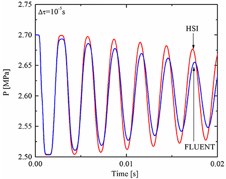
Figure 9. Pressure comparisons of the HSI method and FLUENT at x = 0.2 m under outlet pressure transient using laminar flow model.

FIGURE 10

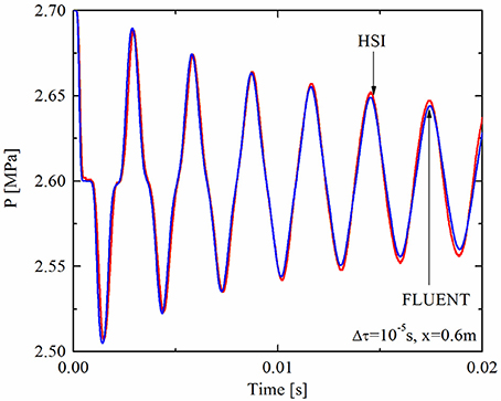
Figure 10. Pressure comparisons of the HSI method and FLUENT under outlet pressure transient using inviscid flow model.

Inlet Mass Flow Transient

The transient condition for inlet mass flow transient is a step increase in inlet mass velocity from 10 kg/(m^2·s) to 20 kg/(m^2·s), and the input parameters are shown in Table 1. For pressure, and temperature responses at x = 0.4 m, the comparisons between FLUENT and the HSI method are shown in Figure 11. It can be seen that the two methods have the same response frequency, while the amplitudes of the HSI method are slightly greater than that of FLUENT. Compared with the pressure transient in Figure 10, the response frequencies of the two transients are the same. There are ~6.5 cycles within 0.02 s for both the pressure transient and mass flow transient. So the mass flow transient is propagated in the same mechanism as the pressure transient at the speed of sound.

FIGURE 11

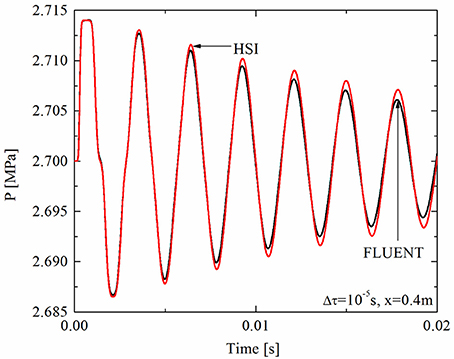
Figure 11. Comparisons of the HSI method and FLUENT under inlet mass flow transient.

Inlet Temperature Transient

The transient condition for inlet temperature transient is a step increase in inlet temperature from 300 to 350°C, and the input parameter settings are shown in Table 1. For the responses of pressure, the mass velocity, and temperature at x = 0.2 m, the results of FLUENT and the HSI method are shown in Figure 12. It can be seen from Figures 12A that a step increase of inlet temperature results in a mild pressure oscillation, whose amplitude is very small (around 1 kPa). The frequency of the pressure oscillation is the same for both FLUENT and the HSI method, while the amplitude of the HSI method is slightly larger than that of FLUENT. Moreover, because pressure and velocity are strongly coupled, the pressure oscillation also leads to the mass velocity oscillation, which has the same frequency as pressure, as seen in Figures 12B. These are fast transients.

FIGURE 12

Figure 12. Comparisons of the HSI method and FLUENT under inlet temperature transient. (A) Pressure responses. (B) Mass velocity responses. (C) Temperature responses.

It can also be seen from Figure 12B that there is a sudden decrease of mass velocity at around τ = 0.04 s, this is a slow transient caused by temperature distribution. At around τ = 0.04 s, the temperature difference signal was transferred to the position x = 0.2 m, as seen in Figure 12C. This causes an increase in local temperature and a decrease in local density. According to continuity Equation (1), the decrease in local density leads to a decrease in the local derivative ∂ρ/∂t, which in turn leads to an increase in local space derivative ∂(ρu)/∂x. For the local control volume, this means that the mass flows out of the volume is greater than that flows into it. As a result, the total local mass flow decreases.

Another phenomenon can be seen from Figure 12B is that the mass velocity of FLUENT first drops to an intermediate value (around 10.3 kg/(m^2·s)) at a steeper rate than that of the HSI method, and then gradually stabilizes at around 10 kg/(m^2·s) with a diminishing oscillation. The mass velocity of the HSI method drops directly to the stable value [10 kg/(m^2·s)] at a slower rate, and then gradually stabilizes with a diminishing oscillation.

There are two reasons for this phenomenon. First, FLUENT uses a second upwind scheme while the HSI method used a first upwind scheme, so the solution of FLUENT is more accurate than the HSI method, and the temperature distribution is steeper, as seen in Figure 12C. This in turn contributes to a steeper decrease of mass velocity in FLUENT. Second, because FLUENT used a two-dimensional laminar flow model, the velocity is zero at the wall and maximum at radial center. This velocity profile leads to the temperature distribution in Figure 13, which illustrates the average axial temperature distribution of FLUENT and the HSI method at τ = 0.1 s.

FIGURE 13

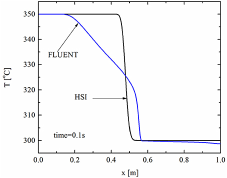
Figure 13. Average axial temperature distribution of the HSI method and FLUENT at time = 0.1 s under inlet temperature transient.

As a result, local temperature changes very quickly in the beginning and then gradually slows down, as shown in Figure 12C. This results in the intermediate value of mass velocity in FLUENT simulation, and its gradual stabilization to the stable value. In the HSI method, an averaged one-dimensional model was employed and the radial temperature profile is uniform. Therefore, the mass velocity of the HSI method directly drops to its stable value when temperature difference signal arrives.

Adaptive Time Step

In order to save computational time, two conditions are considered for adaptive time step in the HSI method to speed up calculations, namely the maximum relative density difference between the two densities (one by continuity equation and the other by state equation), and the Courant–Friedrichs–Lewy (CFL) condition.

Maximum Relative Density Difference

The maximum relative density difference is

$\begin{array}{cc}\Delta {\rho }_{\max }=\underset{i=1}{\stackrel{N}{\max }}\left(\frac{\left|{\rho }_{i,1}^{n+1}-{\rho }_{i,2}^{n+1}\right|}{{\rho }_{i,2}^{n+1}}\right)& \left(17\right)\end{array}$

In which ρ₁ is solved implicitly using the continuity equation and ρ₂ is solved by state equation. Δρ_max is the maximum relative density difference between ρ₁ and ρ₂. If Δρ_max ≤ Δρ_L (the lower limit of Δρ_max), then the errors under this time step are small enough to allow greater time step for faster calculation while still retaining high accuracy. On the other hand, if Δρ_max > Δρ_H (Δρ_H is the upper limit of Δρ_max), then the relative density error may be too large to converge, and the time step should decrease to ensure convergence. Based on the a lot of testing, the recommended values of Δρ_L and Δρ_H here are set as Δρ_L = 10⁻⁸ and Δρ_H = 10⁻³ for the HIS method for the transients of the HTRGTS.

CFL Condition

As mentioned in section Maximum Relative Density Difference, a suitable value of Δρ_L saves computational time, and that of Δρ_H ensures convergence. However, the temperature response at x = 0.75 m, as shown in Figure 14, indicates that the solution is unstable under the outlet pressure transient condition.

FIGURE 14

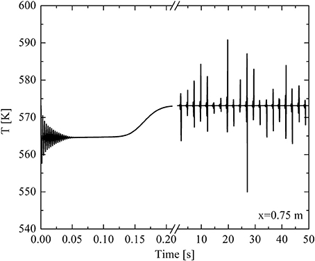
Figure 14. Relationship between temperature and time without considering CFL condition.

To ensure stability, the CFL condition must be considered to control the time step below a certain value, so that the Courant number is lower than its maximum value (c_max). Under a fixed mass velocity of 38.90 kg/(m²·s), the relationship between c_max and the number of nodes under different pipe lengths are shown in Figure 15. It can be seen that (1) the value of c_max decreases with the increase of node number, and (2) c_max was not influenced by pipe length. If the node number is >300, the value of c_max ranges between 1.2 and 1.3. To ensure stability, the value of c_max is set as 1.1 for different node numbers. After the CFL condition was considered, the relationship between time step and time is shown in Figure 16A, and the temperature response at x=0.75 m is shown in Figure 16B. It can be seen from Figure 16A that time step first increased to a certain value and then stabilizes, and a stable solution of temperature is obtained, as seen in Figure 16B.

FIGURE 15

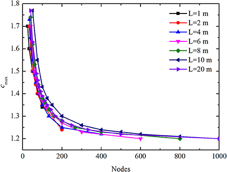
Figure 15. Relationship between c_max and node number under different pipe length.

FIGURE 16

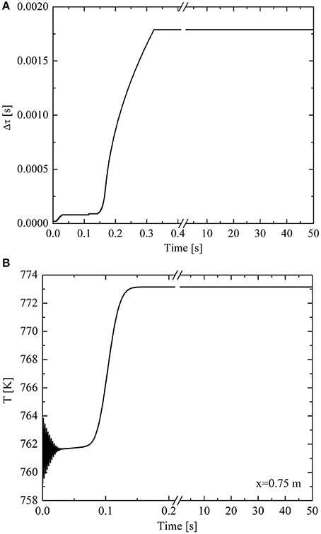
Figure 16. Relationship between time step (A), temperature (B), and time considering CFL condition. (A) Time step. (B) Temperature.

Conclusions

To devise a non-iterative transient solver for one-dimensional compressible flow for high temperature gas cooled reactors gas turbine systems (HTRGTSs), the performance of the semi-implicit and nearly-implicit methods in typical compressible flow transients were studied. The results show that the semi-implicit method can capture the fast pressure responses with little numerical diffusion, but it has poor stability in capturing the slow temperature responses. The nearly-implicit method has good stability in capturing temperature responses, but it has too great numerical diffusion in capturing pressure responses.

Based on the discussion of the two methods, a new HSI method that combines the advantages of both the semi-implicit and nearly implicit methods was proposed. In the HSI method, a new calculation strategy is devised: the convective term in momentum equation is treated explicitly to solve pressure and velocity; density and temperature are solved implicitly using continuity and energy equations.

The HSI method was verified via the shock tube benchmark problem, and furtherly compared with FLUENT simulations. In verification with the shock tube benchmark problem, it was found that the HSI method can capture pressure transient accurately, and there are no spurious oscillations at the pressure step change points. In comparisons with FLUENT simulations, the outlet pressure transient, inlet mass flow transient, and inlet temperature transient were studied. The results show that the response frequencies of the HSI method are the same as those of the FLUENT simulations, while the amplitudes of the HSI method are slightly larger than those of FLUENT simulations. The HSI method is capable of capturing both the fast transients (such as pressure transient), and the slow transients (such as temperature transient) with good accuracy.

An adaptive time step scheme was furtherly proposed for faster calculations of the HIS method while still retaining a good convergence, stability, and accuracy. Two conditions are considered in this scheme, namely the maximum relative density difference, whose upper limit is set as 10⁻³ and lower limit 10⁻⁹, and the CFL condition, in which the maximum Courant number is set as 1.1.

Author Contributions

XC and MD contributed to the conception of the study. ZM contributed significantly to analysis and manuscript preparation. JW performed the data analyses and wrote the manuscript. JW helped perform the analysis with constructive discussions.

Conflict of Interest Statement

The authors declare that the research was conducted in the absence of any commercial or financial relationships that could be construed as a potential conflict of interest.

Nomenclature

ρ, u, T, P: density, velocity, temperature and pressure, respectively; Δτ, Δx: time step and space step, respectively; c_v: specific heat capacity of helium under constant volume; f_w: frictional factor; c_m: averaged factor when 3D flow is integrated and averaged to 1D flow; D_e, A_c: hydraulic diameter and cross Sec. area of the pipe; E, c, d, r, l, A, B, C, D, a_p, a_w, a_e: coefficients used to simplify calculation; Superscript ”~”: intermediate time variable; Superscript “.”: the donored value at cell face; Superscript “ⁿ ”: value of last time step; Superscript “ⁿ⁺¹ ”: value of this time step; subscripts K, L, M: cell center i-1/2, i+1/2 and i+3/2, respectively.

References

Bentivoglio, F., Tauveron, N., Geffraye, G., and Gentner, H. (2008). Validation of the CATHARE2 code against experimental data from Brayton-cycle plants. Nuclear Eng. Design 238, 3145–3159. doi: 10.1016/j.nucengdes.2007.12.026

CrossRef Full Text | Google Scholar

Bestion, D. (2008). System Code Models and Capabilities, in THICKET-2008. University of Pisa (UNIPI), Italy.

Google Scholar

Division, N. S. A. (2001). Relap5/mod3.3 Code Manual Vol. 1. Washington, DC: U. S. Nuclear Regulatory Commission.

Greyvenstein, G. P. (2002). An implicit method for the analysis of transient flows in pipe networks. Int. J. Num. Methods Eng. 53, 1127–1143. doi: 10.1002/nme.323

CrossRef Full Text | Google Scholar

Patankar, S. V. (1980). “Numerical heat transfer and fluid flow,” in Computational Methods in Mechanics and Thermal Science, ed E. M. S. W. J. Minkowycz (Washington, DC; New York, NY; London: McGraw-Hill Inc), 126–130.

Rousseau, P. G., du Toit, C. G., and Landman, W. A. (2006). Validation of a transient thermal-fluid systems CFD model for a packed bed high temperature gas-cooled nuclear reactor. Nuclear Eng. Design 236, 555–564. doi: 10.1016/j.nucengdes.2005.11.016

CrossRef Full Text | Google Scholar

Saez, M., Tauveron, N., Chataing, T., Geffraye, G., Briottet, L., and Alborghetti, N. (2006). Analysis of the turbine deblading in an HTGR with the CATHARE code. Nuclear Eng. Design 236, 574–586. doi: 10.1016/j.nucengdes.2005.10.025

CrossRef Full Text | Google Scholar

Tao, W. (2001). Numerical Heat Transfer. Xi'an: Xi'an Jiaotong University Press.

Google Scholar

Toro, E. F. (2009). Riemann Solvers and Numerical Methods for Fluid Dynamics, 3rd Edn. Dordrecht; Heidelberg; London; New York, NY: Springer. 115.

van Ravenswaay, J. P., Greyvenstein, G. P., van Niekerk, W. M. K., and Labuschagne, J. T. (2006). Verification and validation of the HTGR systems CFD code flownex. Nucl. Eng. Design 236, 491–501. doi: 10.1016/j.nucengdes.2005.11.025

CrossRef Full Text | Google Scholar

Widlund, O., Geffraye, G., Bentivoglio, F., Messié, A, Ruby, A., Saez, M., et al. (2005). “Overview of gas cooled reactor applications with CATHARE,” in The 11th International Topical Meeting on Nuclear Reactor Thermal-Hydraulics (NURETH-11) (Avignon; Popes Palace Conference Center).

Yan, X. (1990). Dynamic Analysis and Control System Design for an Advanced Nuclear Gas Turbine. Dept. of Mechanical Engineering; Massachusetts institute of Technology: Massachusetts Institute of Technology.

Google Scholar