 Tengfei Wei
 Yiyang Wang
 Jichang Yang
- School of Electrical and Information Engineering, Lanzhou University of Technology, Lanzhou, China
With the rapid development and increased demand for renewable energy sources, standalone hybrid generation systems have become an essential energy solution. Power optimization control is thus critical to achieving the efficient operation and stability of this system. The distributed ADMM (alternating direction method of multipliers)-based approach has the full potential to deal with the power optimization problem of standalone hybrid generation systems. This study uses an optimization algorithm with a Gaussian penalty function, ADMM-ρ, to alternately optimize the power reference values of wind, light, and battery-containing power generation subsystems. The local controller regulates the output power of the converter according to this reference value. This ensures that the wind and photovoltaic power generation subsystem work in load-tracking or maximum power-tracking modes so that the optimal operation of hybrid power generation meets the balance of supply and demand while prolonging the service life of the batteries. Simulation experiments show that the distributed ADMM algorithm can reliably address the power optimization challenge of hybrid power generation systems.
1 Introduction
Due to current problems of environmental pollution and energy scarcity, wind and solar energy, rich in reserves, have attracted more attention as crucial clean energy sources to effectively cope with the energy crisis and environmental problems (Suo et al., 2021). In order to meet the balance between power generation and the load power of off-grid hybrid systems, maximizing the use of clean energy resources while considering and extending battery service life can make a whole system operate more efficiently and reduce operating costs; the key is the optimal power distribution of each power generation unit. Therefore, much research has studied the optimal power allocation of standalone hybrid generation systems. Feroldi and Zumoffen (2014) optimized the control of the operating mode of each generating unit of a standalone hybrid wind, solar, and storage power generation system to ensure power balance between the generating units and the loads. Feroldi et al. (2015) proposed an optimal management strategy for batteries in power generation systems that can consider a battery’s state of charge between reasonable upper and lower limits to ensure that it does not overshoot and over-discharge to prolong its service life and ensure its safe operation. Zhao and Yuan (2016) proposed a fruit fly optimization algorithm based on power optimization allocation control to achieve multi-objective optimization with the simultaneous minimization of annual power generation costs and CO2 emissions. Wang et al. (2017a) used a hierarchical control structure with distributed predictive control to achieve optimal power allocation in standalone hybrid generation systems to reduce the time cost associated with centralized optimal control and satisfy the system’s power balance. Le et al. (2020) reviewed the current status and development of research on distributed model predictive controls applied in hybrid power system. Considering the power balance, output power of each power generation unit, battery state of charge, and other factors in the objective function, distributed model predictive control can optimize the output power of the coordinated multiple power generation units to achieve optimal functioning to maximize a whole hybrid power generation system’s use of wind and clean energy while prolonging battery life to further improve the operating efficiency of the system and reduce operating costs.
For standalone hybrid generation systems that contain multiple types of generation units, centralized model predictive control can be used to study power optimal control problems. However, this method involves significant computation and high communication and time costs to find an optimal solution while exposing the information on each generation unit. The current approach is inadequate for protecting the privacy of a generation unit’s information. To address this issue, ADMM utilizes its decomposability and fast convergence to break down large-scale and complex optimization problems into smaller sub-optimization problems. Each sub-optimization task is processed in parallel on a corresponding computing node, utilizing coordination and cooperation among the sub-optimization tasks to enhance the efficiency of the optimization computation. However, it is important to note that ADMM may be influenced by the specific characteristics of problems and parameter selection. To address this limitation, this paper introduces a Gaussian penalty function that enhances the power optimization performance of the system by improving convergence speed.
Currently, the standard distributed optimization methods are the gradient descent method (Bottou et al., 2018), the proximal gradient descent method (Parikh, 2014), the coordinate descent method (Wright, 2015), and the alternating direction method of multipliers (ADMM). Among these, ADMM combines the advantages of decomposability and fast convergence of the multiplier method. In hybrid power generation systems, ADMM can decompose the power optimization problem of each power generation unit and, under its constraints, first solve it locally, then update the parameters in the rest of the power generation units, and finally make the hybrid power generation system work in the optimal state through the above iterations; the multiplier method in ADMM can better solve the contradiction between the good convergence of small step lengths and the non-convergence of considerable step lengths (Y. Wang et al., 2017b). It thus ensures the fast convergence of a power generation system (Chang et al., 2019). Increasing the penalty function can increase the maximum iteration step length compared with the gradient descent method, which can accelerate convergence speed (Chang et al., 2019). ADMM is thus suitable for wind–solar–storage hybrid power generation systems, which present a power optimal control problem containing multiple generation types; by improving the ADMM algorithm to increase convergence speed, it can improve the performance of power optimal control of a hybrid power generation system (Kang et al., 2018).
We here establish mathematical models for the subsystems of wind power generation, photovoltaic generation, and batteries. We apply the ADMM algorithm to establish the objective function and constraints. The convergence speed of the ADMM algorithm is enhanced by introducing the Gaussian penalty function ρ. The resulting ADMM-ρ algorithm is used to determine power reference values for wind power generation, photovoltaic power generation, and battery subsystems. The power reference values are alternately optimized, and by modifying the converter’s output power, the wind and PV power generation systems operate in load tracking or maximum power tracking mode. This results in the hybrid power generation system’s optimal operation, ensuring the balance between supply and demand while prolonging the battery’s service life.
This paper is organized as follows. Section 2 offers a mathematical model for standalone hybrid generation systems. Section 3 discusses the ADMM power optimal control framework for these systems, including the power optimization process, objective function, constraints of the ADMM optimization, and iterative design of the distributed ADMM-ρ. Section 4 presents a simulation experiment utilizing WP data from a southern region of China, with load power serving as the input to simulate the proposed model. The results of the simulation experiment are then analyzed.
2 Mathematical modeling of standalone hybrid generation systems
Standalone hybrid generation systems consist of three subsystems: wind power generation, photovoltaic power generation, and battery (Figure 1).
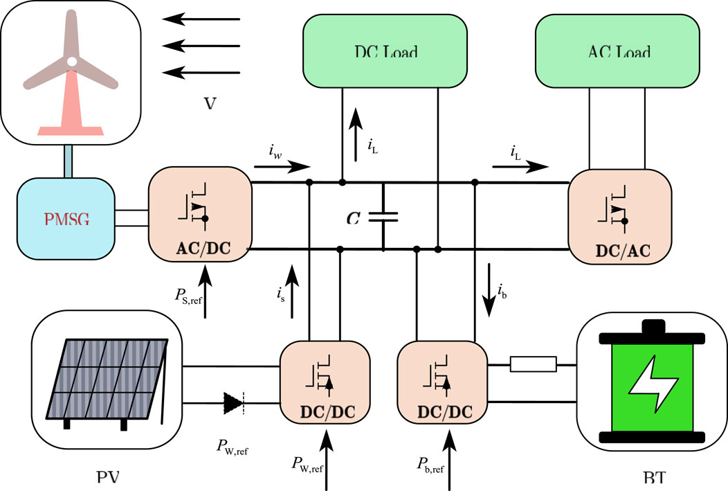
FIGURE 1. Topology of off-grid hybrid power generation system topology.
The photovoltaic power generation subsystem is composed of wind turbines, permanent magnet synchronous generators (PMSGs), rectifiers, and DC/DC converters. Battery subsystems are the energy storage devices of hybrid power generation systems which are composed of batteries and DC/DC converters. The three subsystems operate in parallel via the DC buses to supply power to the DC loads, or through the inverter to supply power to the AC loads.
2.1 Wind electronic system model
Wind power is generated by a wind turbine that absorbs wind energy and converts it into mechanical energy in the drive chain. A generator then converts the mechanical energy into electrical energy to supply the load. According to the principle of aerodynamics, the expression of the output power of a wind turbine is expressed as follows:
where ρ is the air density,
where
The mathematical model of a permanent magnet synchronous generator in the DC coordinate system is established as follows:
where
Eq. 3 is rewritten as follows:
where
Considering that the rectifier and DC/DC converter will have a power loss of about 5% (Xin et al., 2019), the expression for the power flowing from the wind power generation subsystems to the DC bus is represented as follows:
2.2 Model of the photovoltaic power generation subsystem
The model of photovoltaic power generation subsystem is as follows:
where
Eq. 7 can be rewritten as follows:
where
Considering that the power loss of the converter is around 5%, the equation for the power flowing from the photovoltaic power generation subsystems to the DC bus is represented as follows:
From (7) and (9), the power of the photovoltaic power generation subsystems is controlled by
2.3 Model of battery subsystems
Power from wind generation quickly fluctuates due to external influences; the battery subsystems, as energy storage devices (Tan et al., 2021), can quickly respond to the power changes of the wind power generation subsystems and loads. The current flowing through the battery subsystems for power generation is represented as follows:
where
where
Eq. 12 can be rewritten as follows:
where
3 ADMM power optimal control for standalone hybrid generation systems with wind power and storage
Under weather conditions and load variations, the subsystems of standalone hybrid generation systems calculate the output power reference values of the wind, light, and battery subsystems through the ADMM alternately and iteratively and pass the output power reference values to the local controller of these subsystems. This adopts the sliding-mode variable-structure control to change the duty cycle of the DC/DC converter and adjusts the output power of the wind, light, and battery subsystems to meet the user’s load power requirements. The local controller uses a sliding mode variable structure control to change the duty cycle of the DC/DC converter to adjust the output power of the wind, light, and battery generation subsystems so that the output power of the hybrid generation systems meets the user’s load power demand. We thus obtain the ADMM control structure of the standalone hybrid generation systems (Figure 2). The power reference values of the wind, PV, and battery subsystems are used as decision quantities, which are solved by the ADMM algorithm in distributed iterations. The fast convergence of the algorithm is ensured by adding Gaussian penalty variables.
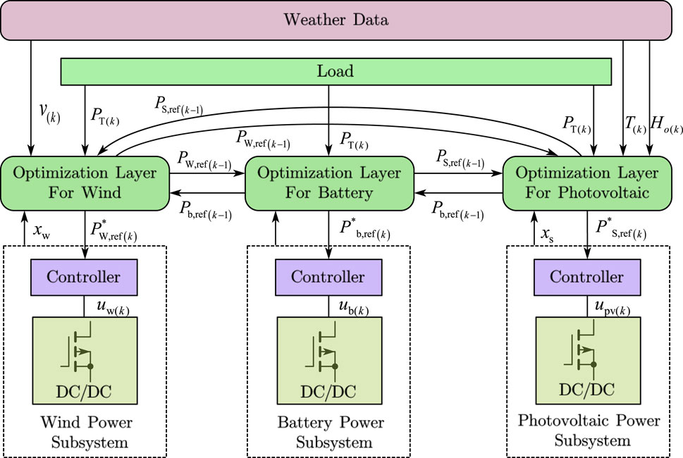
FIGURE 2. Block diagram of the ADMM control structure for the off-grid hybrid power generation system.
3.1 ADMM control structure for standalone hybrid generation systems
The structural block diagram of ADMM-based hybrid power generation system control is shown in Figure 2, where the ADMM power optimization of the wind, photovoltaic, and battery subsystems constitutes the optimization layer, and the optimization layer outputs the reference power to the local controllers of these subsystems.
The objective function of the system optimization layer is first designed. Then, the ADMM optimization algorithm is applied to the wind, PV, and battery power references with alternating iterations based on historical weather prediction data (WP), including light intensity
Finally, the power reference values of the last iteration are exchanged among wind, PV, and battery, the residuals are calculated, and the residual convergence conditions are judged to obtain the optimal power reference values
The optimization layer sends the optimal power reference values
3.2 ADMM distributed power optimization process
Traditional centralized optimization accepts all state information. It makes the optimal control decision of the system, while distributed ADMM performs local optimization for each subsystem and achieves global optimization through iterative optimization among subsystems.
Define
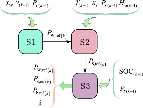
FIGURE 3. ADMM distributed computing framework.
The steps for solving for ADMM-
Step 1:. S1 starts solving the
Step 2:. S1 passes the calculated value of
Step 3:. S2 solves the power reference value of the photovoltaic power generation subsystems
Step 4:. S2 passes the value of the calculation result
Step 5:. S3 solves the predicted value of the power reference for the battery subsystems
Step 6:. S3 passes the value of the calculation result
Step 7:. Solves
Step 8:. Update the value of
3.3 ADMM optimization objective function and constraints
The quadratic objective function for the wind power generation subsystems is represented as follows:
where
The objective function of the photovoltaic power generation subsystems is as follows:
where
The constraints of the photovoltaic power generation subsystems are as follows:
The objective function of the battery subsystems is expressed as follows:
where
The constraints for the battery subsystems are as follows:
x indicates that the optimization objective vector is represented as follows:
According to (14), (16), and (18), the whole system’s optimization objective function is as follows:
where H is the coefficient matrix of the global optimization objective function of the system, which is a semi-positive definite symmetric matrix if the value of the diagonal element is immense. The corresponding wind power reference value, photovoltaic power reference value, or battery power reference value will have a more significant impact on the objective function.
3.4 Distributed ADMM-ρ iterative design
The ADMM-ρ is used to solve the power references
Define the auxiliary variable
where dorm
The augmented Lagrangian function for constructing each suboptimization problem is as follows:
where
The iterative calculation order is
where the penalty coefficient
When
The size of the penalty region is characterized by the parameter
When
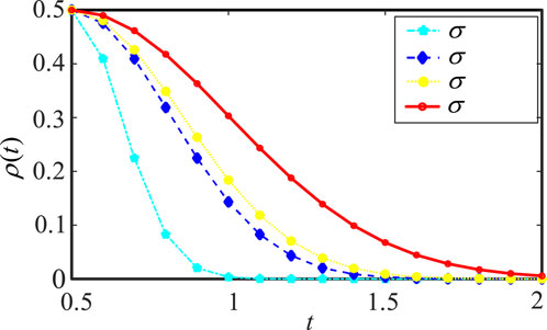
FIGURE 4. Whenβ=0.5 and v=0.5, the variation curve of the penalty function.
The change of the penalty function
Convergence criteria:
where
The flowchart of ADMM algorithm optimization is shown in Figure 5.
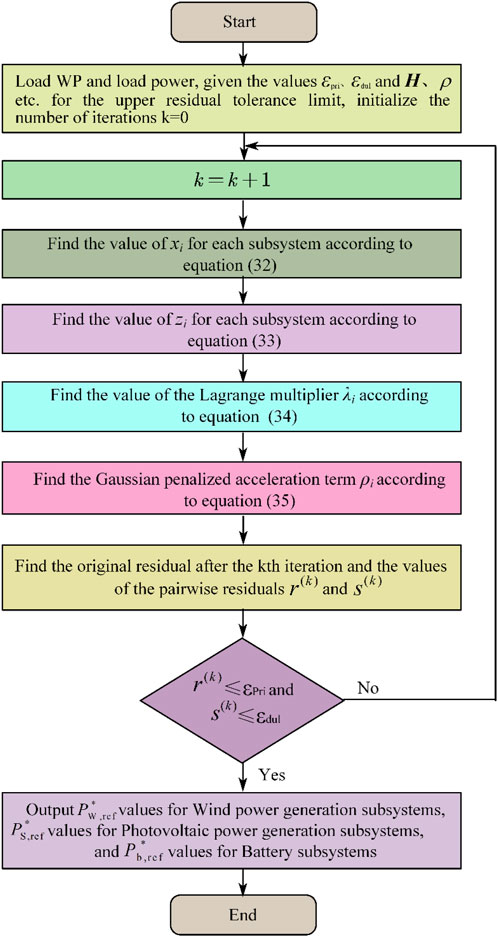
FIGURE 5. ADMM-ρ Optimization flowchart.
The specific process of ADMM-ρ iterative optimization is as follows.
(1) Load the WP data, SOC data, and load power; initialize parameters such as H, ξ,
(2) k=k+1;
(3) Wind power generation subsystems are subjected to the k-times iteration, solving
(4) Wind power generation subsystems pass the calculation results
(5) Photovoltaic power generation subsystems are subjected to the k times iteration, solving
(6) The photovoltaic power generation subsystems transfer the calculation results
(7) Battery subsystems are subjected to the k times iteration, solving
(8) The battery subsystems pass the k sub-corrected value to the photovoltaic power generation subsystems through the contact line.
(9) The photovoltaic power generation subsystems pass the k sub-corrected values to the wind power generation subsystems through the contact line.
(10) The photovoltaic power generation subsystems pass the k sub-corrected values to the wind power generation subsystems through the contact line.
(11) Calculate the values of residuals
(12) Compare whether
4 Simulation verification and result analysis
4.1 Experimental data
In this paper, the WP data and load power for a day in a region in southern China are selected as the inputs to the system (Figure 6): As shown in Figure 6A, the temperature range is 6 °C–17 °C. As shown in Figure 6E, the range of light intensity is 0.002–700 W/
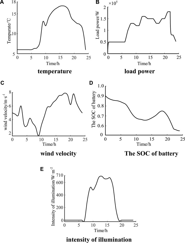
FIGURE 6. Input of the system.
4.2 Simulation results
The standalone wind and storage hybrid power generation system is simulated, and 24 h are selected as the simulation time. The power of the wind and photovoltaic power generation subsystems and the power and current of the battery subsystems are shown in Figure 7.
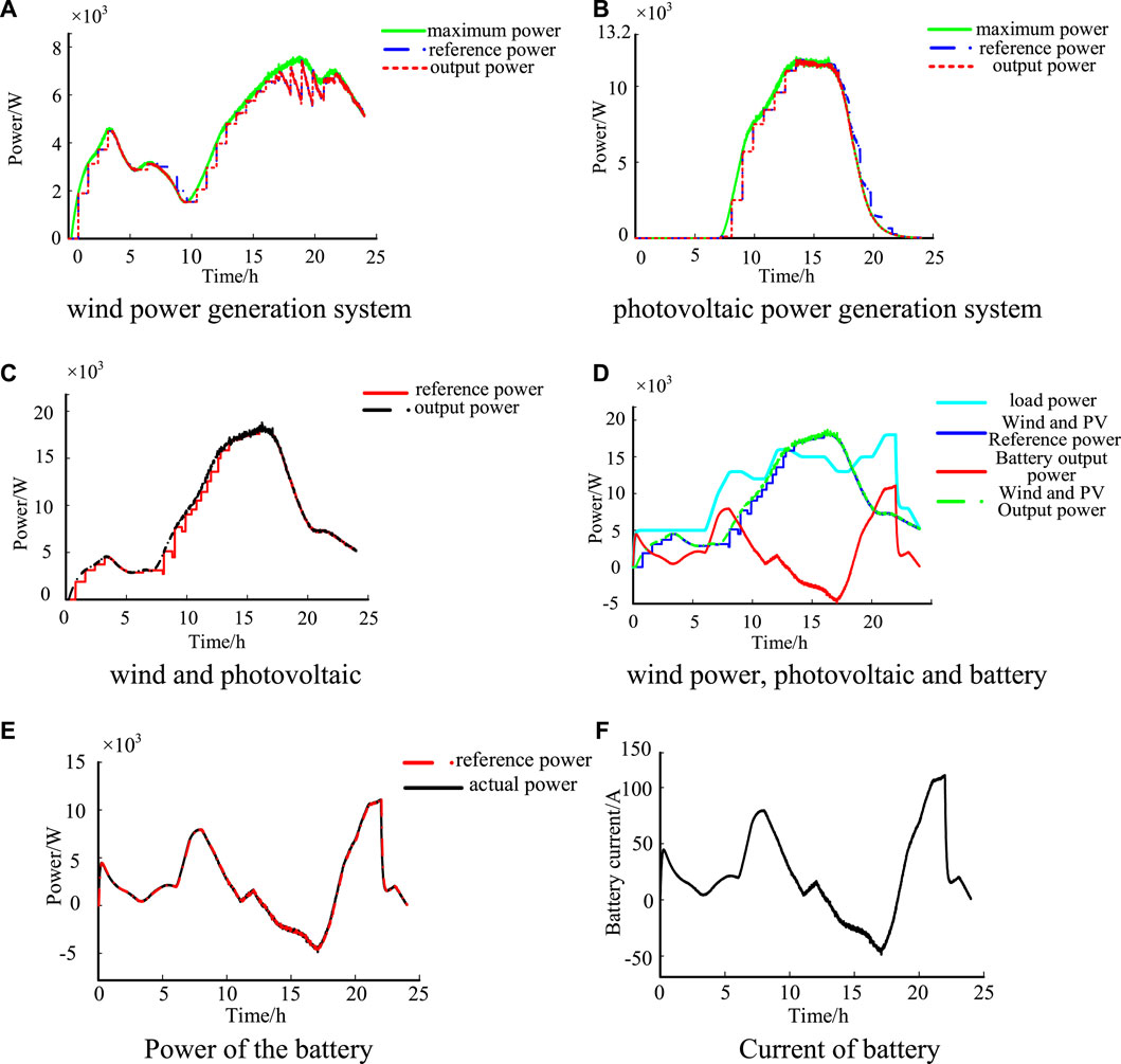
FIGURE 7. Output power of the system and the battery current.
Take 21:00-22:00 in 24 h as an example. The load power is a constant value of 18kW, the reference power range of the wind power generation subsystems obtained by the ADMM solution is 6716.0–6697.0 W, the reference power range of the photovoltaic power generation subsystems is 262.6–654.9 W, and the total output reference power range of the wind and photovoltaic power generation subsystems is 6978.6–7351.9 W. However, the total output actual power range of the wind and photovoltaic power generation subsystems is 7303.0–6987.0 W, the wind and photovoltaic subsystems cannot satisfy the power demand of the load, the battery subsystems have an output power of 10,697.0–11013.0 W, and the controller adjusts the duty cycle of the converter so that the battery subsystems are all working in maximum power tracking from 21:00-22:00 mode so that the battery is in a discharged state. The whole system is in an insufficient state over 21:00–22:00. According to the simulation results, during 0–24 h, the system is in a sufficient state in the phase 12:00–18:00, in a balanced state in the phase 12:00–18:00, and in a deficient state in the phases 0:00–12:00 and 18:00–24:00. During 12:00–18:00, the wind power and photovoltaic power generation subsystems are working in the load tracking mode in which the battery absorbs excess power. For 0:00–12:00 and 18:00–24:00, the wind and photovoltaic power generation subsystems are operating in maximum power tracking mode, and the battery subsystems make up the difference in power to stabilize the system.
Figure 7E shows the power curve of the battery; the positive power indicates that the battery is discharging, and the negative power indicates that the battery is charging. Due to the rapid response of the battery, its actual power value curve coincides with the power reference value curve, which ensures the stable operation of the system. Figure 7A shows the maximum, reference and output power of wind power systems; Figure 7B shows the maximum, reference and output power of the PV systems; Figure 7C shows the reference power and output power of wind and PV; Figure 7D shows the actual output power of wind, PV and battery, load power.
Figure 7F shows the current waveform of the battery; the current is positive battery discharging, and the current is negative battery charging. At 0:00–12:00 and 18:00–24:00, the battery is discharging, and at 12:00–18:00, the battery is charging.
4.3 Convergence analysis of the ADMM algorithm
To ensure that the output power of the hybrid power generation system satisfies the user’s load power demand, the ADMM algorithm must calculate the reference value of the output power of the local controller of the wind, light, and battery subsystems in real-time based on variations in the load and different weather conditions during the simulation process. This calculation alters the duty cycle of the DC/DC converter and adjusts the output power of the wind, light, and battery subsystems. As a result, multiple computations must be conducted to address the issue during the 24-h simulation. Due to space constraints, only the changes in values of the original residuals, pairwise residuals, and convergence thresholds with the number of iterations for a particular calculation are presented. The convergence process of original and pairwise residuals is displayed in Figure 8. As observed, the pairwise residuals attained convergence threshold requirements in the 10th iteration, while the original residuals reached the same in the 14th iteration. The ADMM algorithm exhibits superior capability in finding optimal solutions and achieving convergence speed when addressing the power optimization challenges in standalone hybrid generation systems.
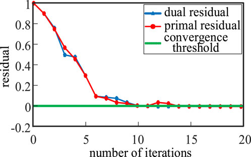
FIGURE 8. Convergence process for primal and dual residuals.
For ADMM and ADMM-ρ with the addition of a Gaussian penalty function, the convergence process of their original residuals is shown in Figure 9. It can be seen that ADMM-ρ reaches convergence the 14th time. This can be compared with ADMM, which is also a distributed optimization, which reaches convergence the 16th time, with ADMM-ρ, which makes the residuals converge to the convergence threshold of 0.001 in a shorter time, and with ADMM-ρ, which has a better convergence characteristic. This improves the optimization ability and convergence speed of the standalone hybrid generation systems for wind, solar, storage, and electricity generation.
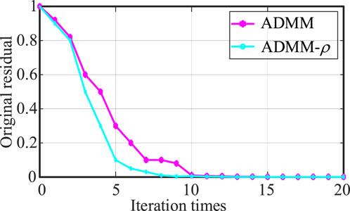
FIGURE 9. Original residual convergence process of ADMM and ADMM-ρ.
5 Conclusion
For the power optimization problem of standalone hybrid generation systems with wind and storage, an ADMM-ρ distributed optimization method based on the Gaussian penalty function is proposed, and the ADMM algorithm is used in the solution of this optimization problem. The ADMM algorithm can make full use of the decomposability of the system to solve the multivariate optimization alternately, with good optimization-seeking ability; at the same time, solving the power optimization problem of the standalone hybrid generation systems of wind power and storage is not subject to the limitation of the system size. Finally, the comparison shows that ADMM-ρ with a Gaussian penalty function can converge the residuals to the threshold range more quickly and with better convergence properties than the ADMM method. Power optimal control of standalone hybrid generation systems is a complex and challenging problem. The distributed ADMM approach provides an effective optimization method but still requires further research and improvement to solve various problems in practical applications. Such research can explore aspects such as more efficient information exchange mechanisms, optimization models that consider uncertainty and economics, and integration with energy markets to further improve the performance of optimal power control for standalone hybrid generation systems.
Data availability statement
The original contributions presented in the study are included in the article/Supplementary material; further inquiries can be directed to the corresponding author.
Author contributions
TW: conceptualization, methodology, writing–original draft. YW: validation, writing–review and editing. JY: validation, writing–review and editing.
Funding
The author(s) declare that no financial support was received for the research, authorship, and/or publication of this article.
Conflict of interest
The authors declare that the research was conducted in the absence of any commercial or financial relationships that could be construed as a potential conflict of interest.
Publisher’s note
All claims expressed in this article are solely those of the authors and do not necessarily represent those of their affiliated organizations or those of the publisher, the editors, and the reviewers. Any product that may be evaluated in this article, or claim that may be made by its manufacturer, is not guaranteed or endorsed by the publisher.
References
Bottou, L., Curtis, F. E., and Nocedal, J. (2018). Optimization methods for large-scale machine learning. SIAM Rev. 60 (2), 223–311. doi:10.1137/16M1080173
Chang, X., Liu, S., Zhao, P., and Song, D. (2019). A generalization of linearized alternating direction method of multipliers for solving two-block separable convex programming. J. Comput. Appl. Math. 357, 251–272. doi:10.1016/j.cam.2019.02.028
Feroldi, D., Rullo, P., and Zumoffen, D. (2015). Energy management strategy based on receding horizon for a power hybrid system. Renew. Energy 75, 550–559. doi:10.1016/j.renene.2014.09.056
Feroldi, D., and Zumoffen, D. (2014). Sizing methodology for hybrid systems based on multiple renewable power sources integrated to the energy management strategy. Int. J. Hydrogen Energy 39 (16), 8609–8620. doi:10.1016/j.ijhydene.2014.01.003
Kang, L., Wang, J., Liu, J., and Ye, D. (2018). Survey on parallel and distributed optimization algorithms for scalable machine learning. J. Softw. 29 (1), 109–130. doi:10.13328/j.cnki.jos.005376
Le, J., Liao, X., Zhang, Y.-T., Chang, J.-X., and Lu, J. (2020). Review and prospect on distributed model predictive control method for power system. Automation Electr. Power Syst. 44 (23), 179–191. doi:10.7500/AEPS20200212005
Parikh, N. (2014). Proximal algorithms. Found. Trends® Optim. 1 (3), 127–239. doi:10.1561/2400000003
Suo, X., Zhao, S., Ma, Y., and Dong, L. (2021). New energy wide area complementary planning method for multi-energy power system. IEEE Access 9, 157295–157305. doi:10.1109/ACCESS.2021.3130577
Tan, K. M., Babu, T. S., Ramachandaramurthy, V. K., Kasinathan, P., Solanki, S. G., and Raveendran, S. K. (2021). Empowering smart grid: a comprehensive review of energy storage technology and application with renewable energy integration. J. Energy Storage 39, 102591. doi:10.1016/j.est.2021.102591
Wang, X., Wang, Z., Zhang, X., Bao, G., and Gong, W. (2017a). Distributed predictive control of stand-alone hybrid generation systems. Acta Energiae Solaris Sin. 38 (9), 2403–2411. doi:10.19912/j.0254-0096.2017.09.011
Wang, Y., Wang, S., and Wu, L. (2017b). Distributed optimization approaches for emerging power systems operation: a review. Electr. Power Syst. Res. 144, 127–135. doi:10.1016/j.epsr.2016.11.025
Wright, S. J. (2015). Coordinate descent algorithms. Math. Program. 151 (1), 3–34. doi:10.1007/s10107-015-0892-3
Xin, Y., Chen, W., Sun, R., Shi, Y., Liu, C., Xia, Y., et al. (2019). Analytical switching loss model for GaN-based control switch and synchronous rectifier in low-voltage buck converters. IEEE J. Emerg. Sel. Top. Power Electron. 7 (3), 1485–1495. doi:10.1109/JESTPE.2019.2922389
Keywords: standalone hybrid generation systems, distributed ADMM, power optimal control, renewable energy source, optimal power allocation
Citation: Wei T, Wang Y and Yang J (2024) Distributed ADMM power optimal control for standalone hybrid generation systems. Front. Energy Effic. 2:1337606. doi: 10.3389/fenef.2024.1337606
Received: 13 November 2023; Accepted: 05 January 2024;
Published: 05 February 2024.
Edited by:
Manuel Alcázar-Ortega, Universitat Politècnica de València, SpainReviewed by:
Linfei Yin, Guangxi University, ChinaLina Montuori, Universitat Politècnica de València, Spain
Copyright © 2024 Wei, Wang and Yang. This is an open-access article distributed under the terms of the Creative Commons Attribution License (CC BY). The use, distribution or reproduction in other forums is permitted, provided the original author(s) and the copyright owner(s) are credited and that the original publication in this journal is cited, in accordance with accepted academic practice. No use, distribution or reproduction is permitted which does not comply with these terms.
*Correspondence: Tengfei Wei, dGZ3ZWlAbHV0LmVkdS5jbg==