 Federico Prystupczuk
  Valentín Rigoni
  Alireza Nouri
  Ramy Ali
  Terence O’Donnell
 - UCD Energy Institute, School of Electrical and Electronic Engineering, University College Dublin, Dublin, Ireland
The Hybrid Power Electronic Transformer (HPET) has been proposed as an efficient and economical solution to some of the problems caused by Distributed Energy Resources and new types of loads in existing AC distribution systems. Despite this, the HPET has some limitations on the control it can exert due to its fractionally-rated Power Electronic Converter. Various HPET topologies with different capabilities have been proposed, being necessary to investigate the system benefits that they might provide in possible future scenarios. Adequate HPET models are needed in order to conduct such system-level studies, which are still not covered in the current literature. Consequently, this article presents a methodology to develop power flow models of HPET that facilitate the quantification of controllability requirements for voltage, active power and reactive power. A particular HPET topology composed of a three-phase three-winding Low-Frequency Transformer coupled with a Back-to-Back converter is modeled as an example. The losses in the Back-to-Back converter are represented through efficiency curves that are assigned individually to the two modules. The model performance is illustrated through various power flow simulations that independently quantify voltage regulation and reactive power compensation capabilities for different power ratings of the Power Electronic Converter. In addition, a set of daily simulations were conducted with the HPET supplying a real distribution network modeled in OpenDSS. The results show the HPET losses to be around 1.3 times higher than the conventional transformer losses over the course of the day. The proposed methodology offers enough flexibility to investigate different HPET features, such as power ratings of the Power Electronic Converter, losses, and various strategies for the controlled variables. The contribution of this work is to provide a useful tool that can not only assess and quantify some of the system-level benefits that the HPET can provide, but also allow a network-tailored design of HPETs. The presented model along with the simulation platform were made publicly available.
1 Introduction
The growing presence of distributed generation such as small-scale PV systems, and new types of controllable loads such as electric vehicles (EVs) or electric heat pumps, is increasing the stress on existing distribution systems, creating problems such as voltage rise, thermal overload, higher presence of harmonics and higher system losses (Walling et al., 2008; Procopiou and Ochoa, 2017). Distribution networks have been traditionally designed under the assumption that the only source of power in the grid is the primary substation, and so, the presence of highly variable Distributed Energy Resources (DER) leads to operating situations that were not foreseen in conventional systems (Walling et al., 2008). In this respect, the distribution transformer, one of the most important and robust components operating at the interface between transmission and distribution systems, has limited capabilities to cope with the impact of these new technologies in the electric grid, resulting in potentially increased operational costs and losses (Aeloiza et al., 2003). Augmenting the network with smart and active control appears as a good option to deal with some of the envisaged issues and to potentially mitigate the need for network reinforcement (Bala et al., 2012; Navarro-Espinosa A. and Ochoa L. F., 2015). Nowadays, many of the solutions proposed for achieving a more flexible, controllable and stable grid rely on power electronic devices for their implementation, such as active filters, HVDC, FACTS-devices, electronic breakers, and particularly Power Electronic Transformers (PETs) (Liserre et al., 2016).
The PET is a relatively new device that utilizes power electronic converters to transform electrical power between not only different AC voltage levels but also different frequencies and forms (e.g., AC-DC and DC-AC conversion). Among the several different proposed topologies and implementations of PET, possibly the most researched approach is the three-stage PET due to its high level of controllability and flexibility (Wang et al., 2012; Yang et al., 2016; Ferreira Costa et al., 2017). The PET facilitates new active control functionalities for AC distribution networks in terms of, for example, power flow control, voltage regulation, and limitation of neutral and fault currents, which cannot be implemented by traditional iron-copper Low-Frequency Transformers (LFT) (She et al., 2013; Chen et al., 2019). Also, a more convenient integration of DC distributed generation, battery storage and DC loads becomes possible with the three-stage PET since those devices could be directly connected to the DC ports of the transformer, improving efficiency and reducing costs by eliminating conversion stages (Hunziker and Schulz, 2017). In a broader perspective, the PET offers opportunities for online automated control and decentralized operation in Smart Grids, reducing operational costs and improving the reliability of power systems under highly disruptive complex phenomena such as cascading failures (Pournaras and Espejo-Uribe, 2017).
Besides this, there are important aspects that should be considered when the full PET is compared with the conventional LFT. Although the topologies, control techniques, and technologies applied to the PET design are being continuously improved, its high cost and relatively low efficiency are still some of the problems that this device is facing to be extensively used in the current electric system (Huber and Kolar, 2014). The target maximum efficiency for state-of-the-art PET designs is between 95 and 98%, while for oil-immersed LFTs over 500 kVA it is normally above 99% (She et al., 2013). As a consequence, the Total Cost of Ownership (TCO) of a PET is currently highly unfavourable compared with the TCO of a LFT; the PET capital cost is estimated to be at least five times higher (Huber and Kolar, 2014), and the operation cost is expected to be also increased due to higher maintenance during the PET lifetime.
The hybrid version of the Power Electronic Transformer arises as a possible solution to some of the main limitations that the full PET has in AC grid applications. The Hybrid PET (HPET) is a special type of transformer resulting from the combination of a conventional Low-Frequency Transformer (LFT) with one or more electronic converters. In order to keep the efficiency as high as possible, the electronic converter is designed to process only a fraction of the LFT rated power, providing some level of controllability while the overall efficiency is not considerably affected (Burkard and Biela, 2015; Huber and Kolar, 2019). The capital cost of the HPET is expected to be considerably lower than the PET capital cost and the improved efficiency causes an important decrease in the total losses over the HPET lifetime, resulting in a much more favourable TCO. In addition, in case of a failure in the electronic converter, the HPET has the possibility of bypassing the electronic converter and remaining operational as a conventional transformer, resulting in higher reliability. The previously mentioned advantages make the HPET a viable alternative to the full PET in AC networks. However, clearly because of the reduced rating of the controllable power electronic part, the HPET will have more restrictive limitations on the control it can exert.
Previous works have studied the impact of PETs in LV and MV networks using simplified models in power flow simulations (Guerra and Martinez-Velasco, 2017; Hunziker and Schulz, 2017; Huber and Kolar, 2019). These studies concluded that while the PET is the most convenient option for DC and hybrid grids, it is necessary to further improve the efficiency and reliability for the PET to be a cost-effective alternative in AC systems. In this regard, similar studies could be carried out to investigate the system benefits that different HPET topologies may have in possible future scenarios. However, the development of the models that are necessary for that kind of analysis has not been covered yet in the current HPET literature. To address this gap, this work presents a methodology to develop simplified average power flow models of HPETs, and demonstrates the integration of those models into power flow simulations. These models facilitate the quantification of controllability requirements for voltage, active power and reactive power, becoming a new tool towards the identification of the most beneficial HPET features and topologies.
The proposed methodology has the flexibility to represent important characteristics of the electronic converter which impact at the system level, such as the different power ratings and losses for each of the converters and the various strategies for the controlled variables. By making small changes to the presented model, different circuit configurations and topologies of HPET can be represented, and afterwards tested in power flow simulations of distribution networks models. In this way, the proposed HPET modeling methodology becomes a useful tool not only to assess and quantify some of the system-level benefits that can be obtained with these devices, but also to develop network-tailored designs of HPETs. The developed model along with the simulation platform created to obtain the results presented in this work remain an open-source development in Python, and are freely available for the academic community and distribution utilities (Prystupczuk et al., 2021).
2 HPET Topology and Simulation Tools
2.1 Shunt-Series Combined HPET
In this section, the HPET concept is introduced using a sinusoidal steady-state representation. For the sake of clarity lossless equations are used throughout this section; a representation of the HPET losses will be covered later in Section 3. A single-phase schematic diagram of a shunt-series combined HPET is presented in Figure 1. This shunt-series combined topology consists of the union of two electronic modules in a Back-to-Back (BtB) configuration with a three-winding LFT: Module 1 is electromagnetically coupled to the LFT in a shunt connection with the tertiary winding, while Module 2 is connected in series with the secondary winding.
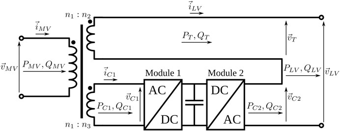
FIGURE 1. Single-phase diagram of HPET with a magnetically-coupled BtB converter.
The shunt-connected DC-AC converter can provide reactive power to the LV grid through the tertiary winding of the LFT. This feature can be utilized for voltage support to the upstream network or for reactive power compensation through reactive power injection, similarly to a D-STATCOM (Liu et al., 2009; Hunziker and Schulz, 2017; Burkard and Biela, 2018). The output voltage of Module 1,
On the other hand, the Voltage-Sourced Converter (VSC) Module 2 is series-connected with the LFT secondary winding, acting as a voltage source that injects a voltage
Where:
SC2max Maximum allowed apparent power of Module 2
STmax Power rating of secondary winding.
Since the combined topology can simultaneously regulate the secondary-side voltage and the primary-side reactive power flow, the ability for reactive power compensation will depend on the actual active power that the electronic converter is instantaneously delivering. This way, the equations for total reactive power compensation in the primary side are the following:
Where:
QC1avail Reactive power available for compensation in Module 1
An alternative HPET shunt-series combined topology can be achieved by using a two-winding LFT with an electronic converted connected in parallel with the secondary winding, as it is shown in Figure 2. In this case, it is necessary to include an injection transformer to adapt the nominal voltage of the electronic converter to the desired series voltage
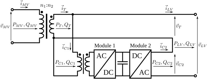
FIGURE 2. Single-phase diagram of the shunt-series combined HPET topology with direct coupling.
2.2 Power Flow Simulations
In order to conduct power flow simulations incorporating the developed HPET models, the Open Distribution System Simulator OpenDSS has been used. This open-source simulation tool can perform almost all the sinusoidal steady-state analyses that are commonly used in distribution systems studies, such as unbalanced multi-phase power flow, quasi-static time-series, fault analysis, harmonic analysis, flicker analysis, etc. A Component Object Model (COM) interface is also provided to facilitate new types of studies and custom solution modes and features from external software. For example, OpenDSS can be entirely driven from external programs written in Python or Matlab, allowing advantage to be taken of all OpenDSS features inside the external software (Dugan and Montenegro, 2020). Consequently, OpenDSS gives the possibility of implementing PET models with different features in a practical and flexible way and analysing their impact in the network using various sinusoidal steady-state analysis tools.
Different types of transformer models are also provided in the OpenDSS platform. While the software offers dedicated definitions for conventional multi-phase multi-winding transformers, different variations can be made by connecting several of these transformers to form a single transformer. For instance, a three-phase transformer can be modeled by using its dedicated definition or also using three single-phase transformers, properly connecting each of their windings. This approach is useful to perform the unconventional series connection of the secondary winding of the HPET in Figure 1 and Figure 2. OpenDSS also provides representation of core and winding losses in the transformer through the parameters %Noloadloss and %Loadloss, respectively. The parameter %Noloadloss represents the percent losses at nominal voltage with no load, and causes a resistive parallel branch to be added in the transformer model. The parameter %Loadloss represents the percent losses at rated load, and adds a percent resistance for each winding on the rated kVA base. The percent magnetising current can be also modeled by using the parameter %imag, which includes an inductance in parallel with the resistive branch that represents core losses. All these parameters are finally embedded within the transformer model as the primitive Y matrix (a nodal admittance formulation of the transformer model), is being computed (Dugan and Montenegro, 2020).
3 Methods. HPET Model for Power Flow Simulations
In this section, the complete development of a sinusoidal steady-state model of a three-phase HPET is presented. The objective of this model is to serve as a tool in power flow studies of distribution systems aimed to assess the capabilities of the HPET from a system-level perspective. This new model has been developed in OpenDSS by implementing the series-shunt combined topology of Figure 1, and builds on the work presented by Guerra and Martinez-Velasco (2017). The schematic diagram of the model is shown in Figure 3 in a three-phase representation. The Back-to-Back converter has been modeled by a combination of a three-phase controlled load and a three-phase controlled voltage source. As it can be seen in Figure 3, the three-phase Load element sets the active and reactive power flows PC1, QC1 in the auxiliary winding, while the Vsource element establishes the magnitude and phase of the voltage Load and Vsource elements are linked by the active power flow, as it is described in Eqs 5, 6. This way, the Load and Vsource elements emulate the behaviour of Module 1 and Module 2 respectively, in the BtB converter of Figure 1. The quantities
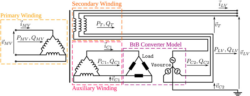
FIGURE 3. Complete three-phase model of the magnetically coupled series-shunt combined HPET.
The three-phase three-winding iron-copper transformer included in the HPET of Figure 3 has been modeled using three single-phase three-winding transformer models in OpenDSS. Those models include a representation of winding and core losses by means of the parameters %LoadLoss and %NoLoadLoss respectively, as well as the transformer percent reactances through the parameters X12, X23 and X13 (Dugan and Montenegro, 2020). In the case of real iron-copper transformers, all those parameters can be normally found in manufacturer specification sheets or catalogs (Siemens, 2017).
One of the key points to be considered in the system-level benefit analysis of HPETs is the converter losses. For this reason, a representation of the electronic converter losses is included in the developed HPET model by assigning an efficiency curve to each of the two electronic modules of Figure 1. The efficiency curve may be a function of different factors, such as load level, temperature, switching frequency, DC-link voltage, etc., depending on the depth needed in the modeling. The load level is the parameter that has the strongest influence on the electronic converter efficiency, and is the one which is considered for the power flow model.
The developed model can deal with bidirectional power flow, where for reverse power the Load element of Figure 3 becomes negative, injecting active power into the transformer (Guerra and Martinez-Velasco, 2017). In Eqs 5, 6, the active power in the electronic converter is respectively expressed for forward and reverse power flow operations. In the same way it was described in Section 2, the reactive power flows QC1 and QC2 of Figure 3 are decoupled between them and can be independently controlled by each module of the electronic converter.
Once the HPET model is integrated into a distribution network model in OpenDSS, a series of calculations must be solved in a sequential way to obtain the solution for each time step, as it is described in the flow diagram of Figure 4. Initially, the Vsource and Load elements are passivated, meaning that Vsource element of Figure 3 according to the adopted voltage regulation strategy. The calculation of the required voltage is implemented as an algorithm in the external software (see Subsection 3.1) and the obtained values are uploaded to the Vsource element configuration in OpenDSS. Then, a new power flow analysis (step 5) is needed to find the new resulting demand and voltages in the circuit. At this point, the PC1, QC1 values for the Load element of Figure 3 are calculated by an algorithm in the external software according to the adopted reactive power compensation strategy (see Subsection 3.2). The calculated PC1 value also account for losses in the electronic converter, obtained through the efficiency model described in Subsection 3.3. A new solution is run in step 7 using the new set points in OpenDSS. Steps 4 to 7 are repeated until the voltage and reactive power relative incremental errors, ϵV and ϵQ respectively, are below a certain limit (0.01 in this case).
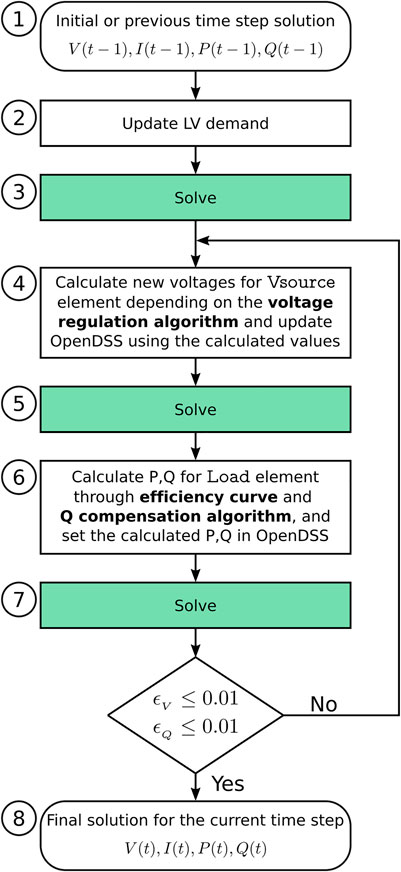
FIGURE 4. Workflow to obtain each time-step solution using the HPET model of Figure 3.
3.1 Voltage Regulation at the Secondary Terminal
In this subsection, the algorithm for regulating the voltage Vsource element (Figure 3) to bring the secondary voltage
Where:
Vsource element for the current time step
Vsource element calculated in the previous time step
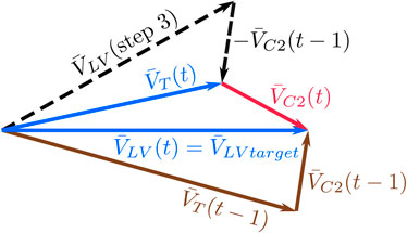
FIGURE 5. Per-phase phasor representation of the output voltage regulation algorithm.
3.2 Reactive Power Compensation
In this subsection, the primary-side reactive power compensation algorithm is described. This algorithm corresponds to the calculations that are performed in step 4 of the flow chart described in Figure 4. The reactive power regulation strategy is aimed to provide compensation in order to maintain unity Displacement Power Factor (DPF) at the primary side whenever it is possible. As it is explained in Section 2.1, the shunt-connected Module 1 (Figure 1) can control QC1 independently from QC2 due to the decoupling provided by the DC-link capacitor. The reactive power available for compensation depends on the power rating SC1max of Module 1 and the actual active power PC1 delivered to the DC-link, as it is described in Eq. 9. In the circuits of Figure 1 and Figure 2, the reactive power injected by the electronic converter should be the negative of the reactive power delivered by the secondary winding in order to compensate reactive power in the primary side, as it is described in Eq. 11.
3.3 Loss Modeling in the Electronic Converter
In most of the corresponding literature, the loss calculation is obtained by multiplying the active power flow by the converter efficiency at the operating point, with the efficiency being a function of the load level and the DPF (Qin and Kimball, 2010; Guerra and Martinez-Velasco, 2017; Rocha et al., 2019; Longo et al., 2020). While this approach can provide accurate results in simulations with high values of DPF, it can lead to unrealistically low losses in situations of low DPF since it only considers the active power flow as the source of losses inside the converter. In the case of the presented HPET model, the Load element of Figure 3 will be operating at a very low DPF most of the time when it is compensating reactive power. Consequently, a different loss modeling approach is needed in this case.
In order to develop a more accurate loss representation that accounts for the loss dependency on the reactive power flow, a three-leg inverter model composed by six VMO1200-01F IXYS power MOSFETs was developed in Matlab/Simulink including the semiconductor losses and thermal model presented by Giroux et al. (2021). A series of simulations were conducted at different load levels, varying the DPF while keeping the load level constant. The obtained results can be observed in Figure 6, where the apparent power Sout delivered by the inverter and the inverter losses Ploss are measured at the different load levels. It can be observed in the resulting curves that the variations for different DPF are negligible, and since at unity DPF the quantity Sout/(Sout + Ploss) is equal to the inverter efficiency, then a single efficiency curve can be used to calculate the input power plus losses, even when the inverter is delivering mostly reactive power. This leads to the loss modeling approach described by Eqs 12–17 and Figure 7 for the case of forward power flow operation.
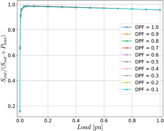
FIGURE 6. Sout/(Sout + Ploss) curves obtained for different DPF at constant apparent power.
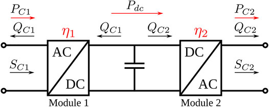
FIGURE 7. Active and Reactive forward power flow operation through the BtB converter.
The presented loss modelling approach has been demonstrated using a MOSFET inverter, but it is also applicable to other types of devices such as IGBTs, due to the nature of losses generated inside the semiconductors. This method contributes a practical way to implement the loss calculation in power flow simulations for any DPF situation using a single efficiency curve, which is usually provided in the datasheet of different power electronics converters.
4 Results
In order to characterize the range of voltage regulation and reactive power compensation capabilities as a function of the PET module rating, two test cases have been carried out, and the corresponding results are shown in this section. In both simulations, an 800 kVA, 10 kV–400 V Hybrid PET is used. In Subsection 4.1, the voltage regulation and reactive power compensation capabilities of the developed HPET model are characterized using the simple setup of Figure 8 in OpenDSS. The simulations consist of independently sweeping
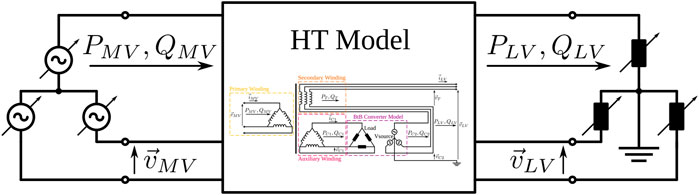
FIGURE 8. Setup in OpenDSS to test the voltage regulation and reactive power compensation capabilities of the developed HPET model.
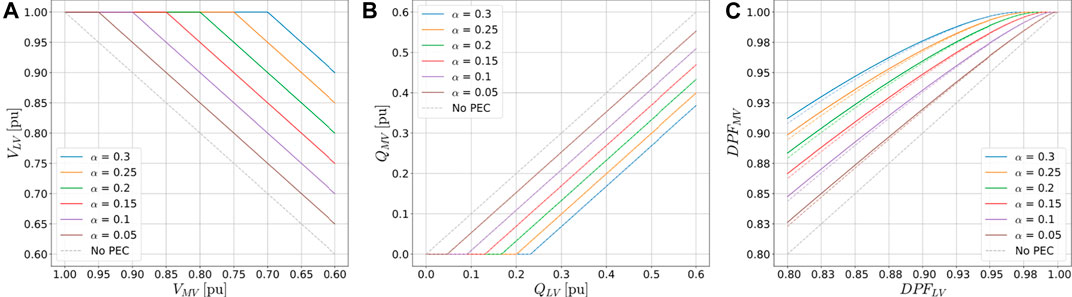
FIGURE 9. Output voltage regulation results in terms of
In Subsection 4.2, a time-series power flow simulation is performed using one of the distribution network models developed by the company Electricity North West and the University of Manchester for the LVNS project, obtained from GIS data of real distribution grids in the north of England (Navarro-Espinosa A. and Ochoa L., 2015). This second simulation has been used to compare the performance of the developed HPET model of Figure 3 with an existing model of PET (Guerra and Martinez-Velasco, 2017) and a conventional LFT model provided in OpenDSS, in terms of voltage regulation, DPF correction, and losses. The models, scripts and all data mentioned in this section used to obtain the presented results are publicly available in the HPET_PowerFlow_Model GitHub repository (Prystupczuk et al., 2021).
4.1 Test Case 1. Standalone Voltage Regulation and Reactive Power Compensation
Using the setup of Figure 8, the voltage regulation algorithm presented in Subsection 3.1 is tested by linearly sweeping the amplitude of
The reactive power compensation algorithm presented in Eq. 11 has been similarly tested by linearly sweeping the reactive power QLV demanded at the secondary terminal from 0.0 to 0.6 pu. In this simulation, the input voltage at the primary side
In Figure 9C, the primary and secondary DPF that result from the sweep simulation are presented, where the measured values (solid lines) are compared with theoretically calculated values (dashed lines) from Eq. 4. In the case of the primary side DPF, PFMV, a difference is observed as a consequence of the losses that are present in the LFT, which cause the DPF in the MV side to be higher due to the higher active power flow. The results obtained in this test case demonstrate that the developed model can effectively and accurately represent the behaviour of a Hybrid PET under a wide range of operating points. They also show in a quantitative way the limitations imposed by the factional power rating of the electronic converter.
4.2 Test Case 2. Power Flow Simulation on a Distribution Network Model
In order to illustrate how the HPET model can be included in a power flow simulation of a distribution network, the network model No 12 developed in the LVNS project has been employed (Navarro-Espinosa A. and Ochoa L., 2015). This test case is aimed at demonstrating the performance of the developed HPET model, as well as at comparing the capability of the HPET for voltage regulation and reactive power control with those of a full PET model presented by Guerra and Martinez-Velasco (2017). The results using a conventional LFT model (no voltage regulation or reactive power compensation) available in OpenDSS are also included for comparison. The technical features of the three used transformer models are shown in Table 1. The utilized network model along with other 24 models of distribution networks are publicly available at Electricity North West (2014).
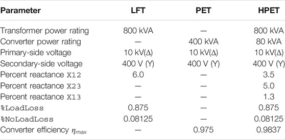
TABLE 1. Parameters used in the different transformer models.
To model PET and HPET losses, the loss model presented in Subsection 3.3 has been used, but the simulated curve of Figure 6 has been replaced by the efficiency curve of a commercially available inverter (Figure 10) for more realistic results. In the case of the HPET, the same curve has been assigned to both Module 1 and Module 2 of the BtB converter (Figure 1), so the resulting BtB efficiency is the product of the efficiency of each Module; e.g., since the curve peak efficiency for the inverter is equal to 0.9918, the peak efficiency of the whole BtB converter is 0.9837. For the full PET, just one curve is used to represent the whole PET efficiency, according to the model presented by Guerra and Martinez-Velasco (2017). But since this is a three-stage device (AD-DC, DC-DC, and DC-AC), a lower efficiency level should be expected and so the curve of Figure 11 has been scaled in order to obtain a peak efficiency of 0.975 for the utilized PET model, which is in accordance with the experimental results obtained by Ferreira Costa et al., 2017.
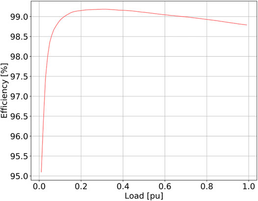
FIGURE 10. Efficiency curve of the 125 kVA KACO Blueplanet 125 TL3 inverter (KACO New Energy, 2021).
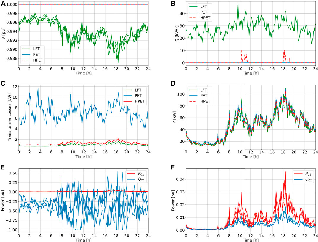
FIGURE 11. Phase-to-neutral voltage VLV at the transformer’s secondary terminal (A). Total reactive power flow QMV at the transformers’ primary terminal (B). Resulting internal losses in the three analysed transformer models (C). Per-phase active power flow PMV through the MV line (D). Active power PC1 and reactive power QC1 set by the Load element (E). Active power PC2 and reactive power QC2 set by the Vsource element (F).
It is important to highlight that for the presented power flow simulation, the LFT and the HPET are rated at 800 kVA, while the PET is rated at 400 kVA. Conventional iron-copper transformers are normally rated based on the peak load method, which considers the highest demand during, for instance, the last year, resulting in oversized transformers that operate most of the time close to their maximum efficiency point (Luze, 2009). In the case of the full PET, adopting the same power rating would imply that the electronic converters will be most of the time operating in the lower part of the efficiency curve, resulting in increased losses in comparison with the LFT. Therefore, by sizing the PET at half the size of the LFT, the load level in this power flow simulation swings between a 15% and an 80% for the PET, and between a 10% and a 40% for the LFT and the HPET cases, approximately.
The LVNS distribution network No. 12, which has been employed to conduct the power flow simulation with the three different transformer models, consisted originally in a radial LV network with 330 residential customers and a single 800 kVA, 10 kV–400 V transformer. In order to allow voltage variations in the primary side of the transformer, the original network has been augmented with a 10 km long MV line that connects the transformer to a substation, indicated in OpenDSS as the slack bus of the system. A set of load profiles consisting of ZIP coefficients with a 5 min resolution, obtained from Rigoni and Keane (2020), are used to model the demand at each time step from each of the 330 customers. The simulation platform used for this second test case has been developed using Python and OpenDSS, building on the Open-DSOPF model presented by Rigoni and Keane (2020). Open-DSOPF is an open-source Python-based model, integrated with OpenDSS, for the formulation of unbalance three-phase optimal power flow problems in distribution grids.
The obtained results can be observed in Figure 11. The voltage at the secondary side of the transformers is plotted per-phase in Figure 11. The adopted strategy for voltage regulation seeks to maintain the secondary voltage at 1 pu, although a different voltage target could be used depending on the needs of the study. As it can be seen, both the PET and HPET models provide perfect voltage regulation over the entire simulation time.
In Figure 11, the resulting reactive power flow in the MV side is shown. The adopted compensation strategy consists in keeping the primary DPF at unity. The green curve shows the total reactive power (i.e., the sum of the three phases) that flows through the MV line when the conventional LFT is used. The PET model provides total reactive power compensation during the whole simulation. On the other hand, the HPET model, equipped with an electronic converter rated at α = 0.1, is not able to compensate the whole reactive power flow at some points in the time series simulation. In those situations, the ability of the HPET to compensate reactive power is limited by the actual active power that is being processed by the electronic converter. The reason for this behaviour is explained in Eq. 9 and can be observed in Figure 11, where the uncompensated reactive power appears at the moments of higher active power drawn by Module 2 (see Figure 11).
The transformer losses and the resulting active power flow in the MV line are respectively presented in Figure 11, respectively. In addition, a computation of energy and losses at different points of the system is presented in Table 2. As expected, the full PET case results in the highest level of losses (around 7.9 times higher than the conventional LFT), while the HPET case results in losses slightly above the losses of the conventional LFT case (around 1.3 times higher), as can be seen in Table 2. The total system losses, i.e., the losses in the distribution transformer plus line losses in the rest of the network, are 3.1 times higher for the PET and 1.1 times higher for the HPET. In Figure 11, the active power flow in the MV line is plotted per-phase, demonstrating the balancing effect of the reactive power compensation from the PET and HPET, and the higher power level that flows through the MV line due to the higher level of losses in the PET.
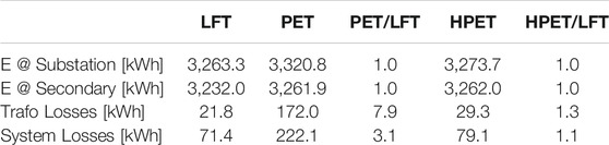
TABLE 2. Resulting computations of energy and losses in the power flow simulation.
Finally, in Figure 11, the active and reactive power flows through Module 1 and Module 2 of the HPET are respectively displayed. As it can be seen, while Module 2 is all the time operating at a very low load level, Module 1 is delivering large amounts of reactive power to keep the primary side DPF at unity. It is evident from Figure 11 that a loss modeling approach that only considers the DPF and the active power flow would not provide an accurate representation of the losses caused by the large reactive currents that take place in Module 1. Hence the need for the proposed loss model presented in Subsection 3.3. It can also be observed in Figure 11 that between the 10th and 12th hours and also between the 18th and 20th hours of the time series simulation, the reactive power compensation of Module 1 reaches its maximum, leading to the red spikes that can be seen in Figure 11. The reactive power compensation capability could be augmented by increasing the power rating of Module 1, with a possible increase in the BtB losses.
The results presented in this section demonstrate the usefulness of the developed model towards the quantification of system-level benefits of including Hybrid Power Electronic Transformers in the distribution system. In this brief example, it can be seen that an HPET equipped with a 10% rated BtB converter can provide voltage regulation and DPF correction to almost the same extent that the full PET, but with considerably lower losses. The power flows presented in Figure 11 show that, in this particular example, there is a large mismatch between the power delivered by Module 1 and Module 2 in the proposed scenario (see Figure 1). This suggests that a possibly optimal BtB configuration may be found by using different power ratings for the two BtB Modules.
Regarding the possible limitations and improvements of the presented HPET model, as it can be seen in the workflow of Figure 4, several power flow snapshots are needed to get one final solution for each time step, possibly making the modeling approach inadequate for long-term studies or high-resolution simulations. A possible improvement that could give faster solutions is to create a custom HPET module in OpenDSS, taking advantage of the open-source nature of the tool by embedding the equations and algorithms described in this work into the OpenDSS public code. This way, the algorithms that represent the HPET behaviour are solved into a single snapshot.
It is also important to mention that further improvements may be done regarding the efficiency modeling of the full PET, since in this presented case an optimistic single efficiency curve is used for the whole device. A more realistic approach would consider a modular implementation of the full PET in which its power rating is allowed to change by enabling and disabling internal modules depending on the actual demanded power (Andresen et al., 2016).
5 Conclusion
Active and smart control in the distribution network appears as a good option to deal with some of the envisaged issues created by the growing presence of distributed generation and new types of controllable loads, which are increasing the stress on the electric grids. There is a growing interest in the possibilities of replacing the passive distribution transformers by active, smart power-electronics-based devices such as Power Electronic Transformers (PETs). However while these devices offer a high level of controllability and flexibility to the network, their cost, losses and reliability are still the main obstacles that prevent their widespread integration into the grid. It is necessary to adequately quantify the net benefits that full and hybrid PETs can provide, using transformers and grid models to conduct simulations in different future network scenarios.
For that reason, a modeling approach of Hybrid Power Electronic Transformers (HPET) for power flow studies is presented in this work along with a new representation of losses in the power electronic converters. The HPET power flow model depicted in Section 3 allows simulating the steady-state behaviour at fundamental frequency of HPETs in the distribution grid, enabling different system-level studies aimed at quantifying the net system benefits. The loss modeling presented in Subsection 3.3 provides accurate results even in cases of low power factor, as well as a practical way of simulating the losses of different converter topologies using a single efficiency curve, that is easily integrated into the presented HPET model.
The presented results demonstrate how the HPET model works under different ranges of voltage, active power and reactive power, as well as how the HPET model, being integrated into a network simulation, facilitates comparisons between different types of transformers. This work contributes a useful tool that allows complete network studies to be conducted, which can quantify the system-level benefits of Hybrid PETs in terms of voltage management, network loss reduction, congestion management and load reduction, and it is freely available as an open-source development (Prystupczuk et al., 2021). Even though the development has been made using OpenDSS, the proposed methodology is valid for any other power flow analysis solver.
Although no harmonic analysis has been included in this work, the harmonic flow analysis is available in OpenDSS, and the developed HPET power flow model is able to handle harmonics. Conducting a harmonic analysis would be not only desirable in order to enhance the load representation, but also to study and quantify the benefits to the system from additional services that could be provided by the HPET, such as harmonics mitigation. That analysis is left for a future study.
Data Availability Statement
The datasets generated for this study can be found in the HPET PowerFlow Model GitHub repository: https://github.com/fprystupczuk/HPET_PowerFlow_Model.
Author Contributions
FP, VR, AN, and TO contributed to conception and design of the study. FP developed the HPET model, developed the inverter loss model, developed the power flow simulation platform and conducted the simulations, and wrote the manuscript. RA developed the Simulink inverter model used in the presented loss model. All authors contributed to manuscript revision, read, and approved the submitted version.
Funding
This work was supported by Science Foundation Ireland under Grant number SFI/16/IA/4496.
Conflict of Interest
The authors declare that the research was conducted in the absence of any commercial or financial relationships that could be construed as a potential conflict of interest.
Publisher’s Note
All claims expressed in this article are solely those of the authors and do not necessarily represent those of their affiliated organizations, or those of the publisher, the editors and the reviewers. Any product that may be evaluated in this article, or claim that may be made by its manufacturer, is not guaranteed or endorsed by the publisher.
References
Aeloiza, E. C., Enjeti, P. N., Morán, L. A., and Pitel, I. (2003). “Next Generation Distribution Transformer: To Address Power Quality for Critical Loads,” in PESC Record - IEEE Annual Power Electronics Specialists Conference, Acapulco, Mexico, 15-19 June 2003, 1266–1271. doi:10.1109/PESC.2003.1216771
Andresen, M., Costa, L. F., Buticchi, G., and Liserre, M. (2016). “Smart Transformer Reliability and Efficiency through Modularity,” in 2016 IEEE 8th International Power Electronics and Motion Control Conference, IPEMC-ECCE Asia 2016, Hefei, China, 22-26 May 2016 (IEEE), 3241–3248. doi:10.1109/IPEMC.2016.7512814
Bala, S., Das, D., Aeloiza, E., Maitra, A., and Rajagopalan, S. (2012). “Hybrid Distribution Transformer: Concept Development and Field Demonstration,” in 2012 IEEE Energy Conversion Congress and Exposition, ECCE 2012, Raleigh, USA, 15-20 Sept. 2012 (IEEE), 4061–4068. doi:10.1109/ECCE.2012.6342271
Burkard, J., and Biela, J. (2015). Evaluation of Topologies and Optimal Design of a Hybrid Distribution Transformer in 2015 17th European Conference on Power Electronics and Applications, EPE-ECCE Europe 2015, Geneva, Switzerland, 8-10 Sept. 2015 (Jointly owned by EPE Association and IEEE PELS), 1–10. doi:10.1109/EPE.2015.7309097
Burkard, J., and Biela, J. (2018). “Hybrid Transformers for Power Quality Enhancements in Distribution Grids - Comparison to Alternative Concepts,” in NEIS 2018; Conference on Sustainable Energy Supply and Energy Storage Systems, Hamburg, Germany, 20-21 Sept. 2018, 1–6.
Chen, J., Yang, T., O'Loughlin, C., and O'Donnell, T. (2019). Neutral Current Minimization Control for Solid State Transformers under Unbalanced Loads in Distribution Systems. IEEE Trans. Ind. Electron. 66, 8253–8262. doi:10.1109/TIE.2018.2883266
Dugan, R., and Montenegro, D. (2020). [Dataset]. Reference Guide. The Open Distribution System Simulator (OpenDSS).
Ferreira Costa, L., De Carne, G., Buticchi, G., and Liserre, M. (2017). The Smart Transformer: A Solid-State Transformer Tailored to Provide Ancillary Services to the Distribution Grid. IEEE Power Electron. Mag. 4, 56–67. doi:10.1109/mpel.2017.2692381
Giroux, P., Sybille, G., and Tremblay, O. (2021). [Dataset]. Loss Calculation in a 3-Phase 3-Level Inverter Using SimPowerSystems and Simscape.
Guerra, G., and Martinez-Velasco, J. A. (2017). A Solid State Transformer Model for Power Flow Calculations. Int. J. Electr. Power Energ. Syst. 89, 40–51. doi:10.1016/j.ijepes.2017.01.005
Huber, J. E., and Kolar, J. W. (2019). Applicability of Solid-State Transformers in Today's and Future Distribution Grids. IEEE Trans. Smart Grid. 10, 317–326. doi:10.1109/TSG.2017.2738610
Huber, J. E., and Kolar, J. W. (2014). “Volume/weight/cost Comparison of a 1MVA 10 kV/400 V Solid-State against a Conventional Low-Frequency Distribution Transformer,” in 2014 IEEE Energy Conversion Congress and Exposition, ECCE 2014, Pittsburgh, PA, USA, 14-18 Sept. 2014 (IEEE), 4545–4552. doi:10.1109/ECCE.2014.6954023
Hunziker, C., and Schulz, N. (2017). Potential of Solid-State Transformers for Grid Optimization in Existing Low-Voltage Grid Environments. Electric Power Syst. Res. 146, 124–131. doi:10.1016/j.epsr.2017.01.024
Liserre, M., Buticchi, G., Andresen, M., De Carne, G., Costa, L. F., and Zou, Z.-X. (2016). The Smart Transformer: Impact on the Electric Grid and Technology Challenges. EEE Ind. Electron. Mag. 10, 46–58. doi:10.1109/mie.2016.2551418
Liu, H., Mao, C., Lu, J., and Wang, D. (2009). Electronic Power Transformer with Supercapacitors Storage Energy System. Electric Power Syst. Res. 79, 1200–1208. doi:10.1016/j.epsr.2009.02.012
Longo, L., Bruno, S., De Carne, G., and Liserre, M. (2020). “Modelling and Performance Evaluation of Smart Transformer in Distribution Grids,” in 2020 IEEE Power & Energy Society General Meeting (PESGM), Montreal, QC, Canada, 2-6 Aug. 2020 (IEEE), 1–5. doi:10.1109/PESGM41954.2020.9281646
Luze, J. D. (2009). “Distribution Transformer Size Optimization by Forecasting Customer Electricity Load,” in 2009 IEEE Rural Electric Power Conference, Fort Collins, CO, USA, 26-29 April 2009 (IEEE). doi:10.1109/REPCON.2009.4919426
Navarro-Espinosa, A., and Ochoa, L. (2015a). Dissemination Document “Low Voltage Networks Models and Low Carbon Technology Profiles”. Manchester: Tech. rep., University of Manchester and ENWL.
Navarro-Espinosa, A., and Ochoa, L. F. (2015b). “Increasing the PV Hosting Capacity of LV Networks: OLTC-Fitted Transformers vs. Reinforcements,” in 2015 IEEE Power and Energy Society Innovative Smart Grid Technologies Conference, ISGT 2015, Washington, DC, USA, 18-20 Feb. 2015 (IEEE), 1–5. doi:10.1109/ISGT.2015.7131856
Pournaras, E., and Espejo-Uribe, J. (2017). Self-Repairable Smart Grids via Online Coordination of Smart Transformers. IEEE Trans. Ind. Inf. 13, 1783–1793. doi:10.1109/TII.2016.2625041
Procopiou, A. T., and Ochoa, L. F. (2017). Voltage Control in PV-Rich LV Networks without Remote Monitoring. IEEE Trans. Power Syst. 32, 1224–1236. doi:10.1109/TPWRS.2016.2591063
Prystupczuk, F., Rigoni, V., Nouri, A., Ali, R., Keane, A., and O’Donnell, T. (2021). [Dataset]. HPET_PowerFlow_Model
Qin, H., and Kimball, J. W. (2010). “A Comparative Efficiency Study of Silicon-Based Solid State Transformers,” in In 2010 IEEE Energy Conversion Congress and Exposition, Atlanta, GA, USA, 12-16 Sept. 2010 (IEEE), 1458–1463. doi:10.1109/ECCE.2010.5618255
Rigoni, V., and Keane, A. (2020). “Open-DSOPF : an Open-Source Optimal Power Flow Formulation Integrated with OpenDSS,” in 2020 IEEE Power & Energy Society General Meeting (PESGM), Montreal, QC, Canada, 2-6 Aug. 2020 (IEEE), 1–5. doi:10.1109/pesgm41954.2020.9282125
Rocha, C., Peppanen, J., Radatz, P., Rylander, M., and Dugan, R. (2019). Inverter Modelling.Tech. rep., EPRI. Palo Alto, CA, United States: Electric Power Research Institute, Inc.
Walling, R. A., Saint, R., Dugan, R. C., Burke, J., and Kojovic, L. A. (2008). Summary of Distributed Resources Impact on Power Delivery Systems. IEEE Trans. Power Deliv. 23, 1636–1644. doi:10.1109/TPWRD.2007.909115
Wang, X., Liu, J., Xu, T., and Wang, X. (2012). “Comparisons of Different Three-Stage Three-phase Cascaded Modular Topologies for Power Electronic Transformer,” in 2012 IEEE Energy Conversion Congress and Exposition (ECCE), Raleigh, NC, USA, 15-20 Sept. 2012 (IEEE), 1420–1425. doi:10.1109/ECCE.2012.6342648
Xu She, X., Huang, A. Q., and Burgos, R. (2013). Review of Solid-State Transformer Technologies and Their Application in Power Distribution Systems. IEEE J. Emerg. Sel. Top. Power Electron. 1, 186–198. doi:10.1109/jestpe.2013.2277917
Yang, T., Meere, R., O'Loughlin, C., and O'Donnell, T. (2016). “Performance of Solid State Transformers under Imbalanced Loads in Distribution Systems,” in 2016 IEEE Applied Power Electronics Conference and Exposition (APEC), Long Beach, CA, USA, 20-24 March 2016 (IEEE), 2629–2636. doi:10.1109/APEC.2016.7468235
Keywords: power electronic transformer, hybrid transformer, power flow simulation, energy distribution systems, transformer losses, inverter losses, power factor
Citation: Prystupczuk F, Rigoni V, Nouri A, Ali R, Keane A and O’Donnell T (2021) Hybrid Power Electronic Transformer Model for System-Level Benefits Quantification in Energy Distribution Systems. Front. Electron. 2:716448. doi: 10.3389/felec.2021.716448
Received: 28 May 2021; Accepted: 19 August 2021;
Published: 14 September 2021.
Edited by:
Yanbo Wang, Aalborg University, DenmarkReviewed by:
Victor Fernão Pires, Instituto Politecnico de Setubal (IPS), PortugalYichao Sun, Nanjing Normal University, China
Copyright © 2021 Prystupczuk , Rigoni , Nouri , Ali , Keane and O’Donnell . This is an open-access article distributed under the terms of the Creative Commons Attribution License (CC BY). The use, distribution or reproduction in other forums is permitted, provided the original author(s) and the copyright owner(s) are credited and that the original publication in this journal is cited, in accordance with accepted academic practice. No use, distribution or reproduction is permitted which does not comply with these terms.
*Correspondence: Federico Prystupczuk , ZmVkZXJpY28ucHJ5c3R1cGN6dWtAdWNkLmll