 Mathias Fontez
 Joris Huguenin2
 Frédéric Jullien
 Sandrine Moja
 Magali Proffit
 Florence Nicole
94% of researchers rate our articles as excellent or good
Learn more about the work of our research integrity team to safeguard the quality of each article we publish.
Find out more
METHODS article
Front. Ecol. Evol., 11 April 2025
Sec. Chemical Ecology
Volume 13 - 2025 | https://doi.org/10.3389/fevo.2025.1536032
Proton Transfer Reaction Time-of-Flight Mass Spectrometry (PTR-TOF-MS) provides high-resolution, real-time tracking of volatile organic compounds (VOCs), yet its analytical workflows for complex mixtures are often underexplored. This study presents a flexible data analysis workflow tailored for PTR-TOF-MS, designed to manage datasets with multiple replicates and experimental factors efficiently. Using lavender plants (Lavandula angustifolia Mill. var. diva) in a controlled greenhouse environment, we analyzed BVOC emissions over a 24-hour cycle. The workflow integrates data importation and optimization via the provoc R package, utilizing Multivariate Curve Resolution (MCR) to decompose spectra into biologically meaningful components and Redundancy Analysis (RDA) to assess component relevance. For this specific model experiment, we determined that normalization using the RUVr method and using and setting the MCR on a number of five components gave the most accurate results. However, this configuration is optimized for the current dataset; other experimental designs may require different normalization methods or numbers of components to achieve optimal results. The workflow enables effective differentiation of VOC emission patterns depending on experimental factors as well as an effective normalization method selection. It provides a systematic approach to PTR-TOF-MS data interpretation, adaptable to various experimental designs and scientific questions, making it valuable for studying complex VOC mixtures in chemical ecology and metabolomics. This method supports long-term, non-destructive sampling while delivering precise VOC profiling.
Biogenic volatile organic compounds (BVOCs) are defined as organic atmospheric trace gases other than carbon dioxide and monoxide, produced by living organisms (Kesselmeier and Staudt, 1999). They represent a high diversity of compounds including isoprenoids, benzenoid, polyketides, fatty acid derivatives. In terrestrial ecosystems, these BVOCs are produced and emitted in the air by a variety of organisms but most of the global total emission is produced by plants and more specifically foliage (Baghi et al., 2012; Greenberg et al., 2012; Dudareva et al., 2013). These fragrant chemicals are produced by plants various organs to interact with their environment. These interactions include plant defense against biotic and abiotic stresses, plant communication, fruit dispersion and pollinator attraction for reproduction (Peñuelas and Staudt, 2010; Abbas et al., 2017).
To understand the functional role of these BVOCs non-destructive approaches are often the most relevant to simulate the ecological environment in which these BVOCs are likely to be involved. The plant is kept alive and undamaged for the duration of the experiment. Under controlled or semi-controlled conditions, an experimental approach is used to vary one or more factors and monitor the resulting variations in BVOCs emissions. These factors can be external biotic factors: introduction of phytophagous insects (Hare, 2011) or pollination (Proffit et al., 2018); external abiotic factors such as light, temperature, hydric status, development stage; and/or internal factors like the circadian clock or developmental stage (Zeng et al., 2017).
In non-destructive approaches, temporal sampling is necessary to measure the effect of the factor(s) on the BVOCs emission. As the plant’s response is not necessarily instantaneous, it is coherent to first establish the temporality of the plant’s response. Similarly, the plant’s response will not necessarily be binary (presence/absence of one compound) but rather quantitative (less/more) and possibly multidimensional (Proffit et al., 2008). Hence, a continuous and non-invasive sampling method is needed.
Till date, temporal and non-destructive sampling of BVOC on plants is still challenging because it is necessary to ensure and control survival conditions (light, air renewal, temperature, air and substrate humidity). The most frequently used non-invasive BVOC sampling techniques are divided into static and dynamic headspace (HS) techniques. Static HS techniques mainly refer to “Headspace Solid Phase Microextraction” (SPME) and can be used for VOC emission timewise sampling. The use of temporal sampling has been previously reported in Agrostis stolonifera and Pennisetum clandestinum, in which the VOCs were collected from plants that were subjected to wounding (Perera et al., 2002). Additionally, it was also used to analyze methyl-salicylate emission by tomato plants after inoculation with tobacco mosaic virus (Deng et al., 2004). SPME sampling was also improved in a time-dependent sampling context, with the adding of an auto-sampler that automatically exposes the fiber to the sample and introduces it into the injection port of the Gas Chromatography coupled with a Mass Spectrometer (GC-MS). This improvement permitted a fine determination of the daily VOC emission pattern of transgenic lines of Arabidopsis thaliana with frequent and regular sampling points over time (Aharoni et al., 2003). This technique is fast and effective however it is not the most appropriate technique for quantitative analysis due to the influence of temperature and sample volume on the adsorption quantity of the fiber (Yang et al., 2013).
On the other hand, dynamic HS techniques were developed on BVOCs in the 80s (Curvers et al., 1984; Mookherjee et al., 1989). Due to the constant gas exchange, this technique avoids the problem of BVOC accumulation in the HS, a challenge often encountered with SPME, and is therefore more suitable for quantitative analysis and tracking continuous variations (Tholl et al., 2020). Thus, it is often preferred over static HS techniques for temporal sampling. For instance, it was used to determine the emission rates of isoprene and monoterpenes of many plant species, sometimes in response to a temperature or a light intensity gradient (Kesselmeier and Staudt, 1999). Several studies also investigate the BVOC emission pattern of a plant after a stress exposure like ozone (Heiden et al., 1999; Dubuisson et al., 2022) or cadmium (Durenne et al., 2018). These techniques are powerful to determine BVOCs’ identity if coupled with MS and to quantify rather precisely. However, depending on the plant species, long sampling time could be a limitation to obtain several acquisition data per day (Cáceres et al., 2016). Furthermore, the sample preparation for dynamic HS extraction is usually delicate and difficult to automatize.
Another non-invasive VOC sampling technique is Proton transfer mass spectrometry (PTR-MS): a sensitive analytical technique that allows for the detection and quantification of trace gases and VOCs in real-time. It was developed in 1998 (Lindinger and Jordan, 1998) by connecting chemical ionization technologies with a flow-drift tube. This technique relies on the chemical ionization by proton transfer reactions with H3O+ ions. The connection to a quadrupole permits the ion m/z analysis. Ion fragmentation is low compared to more classical mass spectrometer techniques, and the time response is very fast because VOCs spend less than 1 second in the drift tube (Tholl et al., 2020). PTR-MS was originally developed for medical purposes like breath analysis, for food research like ripening control and for geophysical research like monitoring changes of VOCs in the ambient air (Lindinger and Jordan, 1998). Subsequently, a PTR-MS with a time-of-flight mass-spectrometer (TOF-MS) was developed, replacing the quadrupole. This modification enables instantaneous detection of whole mass spectra and enhances the separation of single ions according to their m/z ratio (Ennis et al., 2005; Tanimoto et al., 2007). A comparison of the different BVOC sampling methods detailed is shown in Table 1.
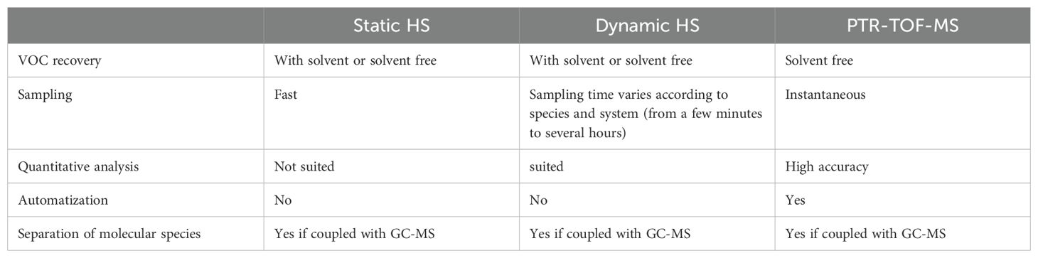
Table 1. Comparison table of different BVOC sampling methods.
The advent of PTR-TOF-MS technology has led to the diversification of the fields of application. Some potential applications are atmospheric VOC analysis (Han et al., 2019; Huang et al., 2020), food analysis like VOC based raspberry cultivar discrimination (Cappellin et al., 2013), Pinot noir wines discrimination (Schueuermann et al., 2017) and fingerprinting of food samples (Cappellin et al., 2012). Similarly, it was used to discriminate wood-cores from different tree species (Taiti et al., 2017). PTR-TOF-MS can also be used to sample BVOC emission at a whole ecosystem level like the global VOC emission and oxidation of a ponderosa pine ecosystem canopy in relation to time and light intensity (Kim et al., 2010; Kaser et al., 2013), or at a whole-year scale: the seasonal changes of BVOC emissions at different heights in the amazon forest (Yáñez-Serrano et al., 2015) and in a Mediterranean oak forest (Yáñez-Serrano et al., 2021). However, studies deploying PTR-TOF-MS to analyze the individual-scale temporal variations of VOCs are relatively scarce. It was used to characterize Arabidopsis thaliana mutants based on VOC emission profile, especially isoprene emission pattern (Li et al., 2020). PTR-TOF-MS was used to determine the accuracy of VOC emission profiles obtained with dynamic chamber systems, testing on timewise VOC emission of Pinus sylvestris shoot (Kolari et al., 2012). Plant VOC emission patterns in relation to external factors were determined using a PTR-TOF-MS for several Mediterranean plants according to development stage (Bracho-Nunez et al., 2011), for Populus alba after wounding and darkening (Brilli et al., 2011), for apple plants after infestation by Pandemis heparana (Giacomuzzi et al., 2016) and for maize leaves according to senescence (Mozaffar et al., 2018) and for inflorescence scent synchrony in Arum maculatum (Marotz-Clausen et al., 2018).
Despite its high accuracy, automation and instantaneity, PTR-TOF-MS is still rarely used in chemical ecology, even though it is particularly well suited for non-invasive temporal sampling of single organism emission. New data-analysis workflows were developed to improve and democratize the use of this technique in the medical field, particularly for the chemical analysis of breath (Roquencourt et al., 2022). However, these workflows are suited for continuous sampling of a limited diversity of compounds and don’t handle experimental designs with replicates and different conditions, as often found in chemical ecology approaches. Firstly, unlike in the classic chromatography analysis, there is no compound separation. All the ions are fragmented together, producing mass spectra corresponding to a sum of parent ions and fragments of all molecules at once. Thereby making the identification of individual compound a difficult process. The issue becomes more acute when the model being studied produces a complex and diverse blend of VOCs. Various strategies have been suggested to overcome this challenge, such as dynamic or static HS intermittent sampling in parallel of the PTR-TOF-MS, or even a direct coupling of PTR-MS with a GC-MS (Lindinger et al., 2005). Our proposal involves resolving these issues by dividing the total fragment ion mass spectrum into sub-spectra associated with conditions that are relevant to the experimenter. Breaking down the total spectrum into groups of masses exhibiting similar behavior under given conditions is another step towards the systematic identification of chemical species. However, this strategy requires the application of an effective normalization process to highlight the trends correctly. This research features several innovative decision-making tools: a normalization selection method employing multivariate redundancy analysis, which is predominantly conducted with visual criteria (Livera et al., 2015; Misra, 2020), or correlation coefficients (Wulff and Mitchell, 2018), and a statistical method capable of dividing a spectrum based on the dynamics of the data (Multivariate Curve Resolution).
In this study we propose a data analysis workflow designed to handle data from PTR-TOF-MS. This workflow aims to efficiently compare samples after normalizing for biological and ecological variability, followed by subsetting the global mass spectra into sub-spectra of molecules that show similar dynamic patterns under experimental conditions, and finally it identifies the effects of the experimental factors. This workflow is designed specially to guide PTR-TOF-MS data analysis in chemical ecology studies with a focus on BVOC emission temporal sampling.
To illustrate our PTR-TOF-MS data analysis process, we used a simple experimental design to sample the BVOC emitted by lavender plants over the period of 24h with two varying discrete factors: day/night and one continuous factor: time, with or without plant. The experiment was carried out in a greenhouse with natural light and a controlled temperature of 20°C at night and 25°C during the day. We used 3-year-old lavender plants (Lavandula angustifolia Mill. var. diva) in full bloom because lavender inflorescences are rich in emitted BVOCs. Plants were chosen to have of the same inflorescence stage, size and inflorescence number. Each plant was placed in a closed cylindrical dynamic chamber (Kolari et al., 2012; see Dubuisson et al., 2022 for more details about the chambers) consisting of a PTFE (polytetrafluoroethylene) disk of 38 cm in diameter, to which a 50µm-thick PTFE transparent film was attached. The chamber’s volume capacity was 30L approximately, and its height could be adjusted according to the size of the plant. The air was purified using a carbon filter before entering the chamber and the flow was maintained at 3 L/min with a flowmeter and an air pump (KNF, N816.1.2K.18R, Germany) for the duration of the experiment. The air inside the chamber was continuously homogenized by a PTFE fan mounted under the disk. The chamber was connected to the pump on one side and to the PTR-TOF-MS on the other, via PTFE tubing. Three independent chambers were measured in one set: 2 chambers containing one plant in a pot and an empty chamber as a control (Figure 1). The PTR-TOF-MS was set to switch chambers every 6min and automatically with a multiway switch. The PTR-TOF-MS sampling time was optimized to have a correct m/z resolution: 30 sec per sampling and 12 sample points per chamber, then the PTRMS switched to the next chamber. All the sample points between 10:30 am and 6 pm are considered “day samples” and all the sample points between 10:30 pm and 6 am are considered “night samples”. Whilst conducting the experiment, the sunset was around 10 pm and sunrise around 6:30 am, the “day samples” could have cover a longer period of time, but in order not to overcomplicate the data, we chose to take a time window of identical length for both day and night. The PTR-TOF-MS m/z parameters were set to cover m/z from 52 to 205. The whole system was set-up 10 hours before for the lavender emission to stabilize and the plant’s evapotranspiration to adapt to the chambers. At the end of each sampling, the inflorescences were cut, dried for one week in a 50°C oven, and weighed. The experiment was performed with 6 biological replicates.
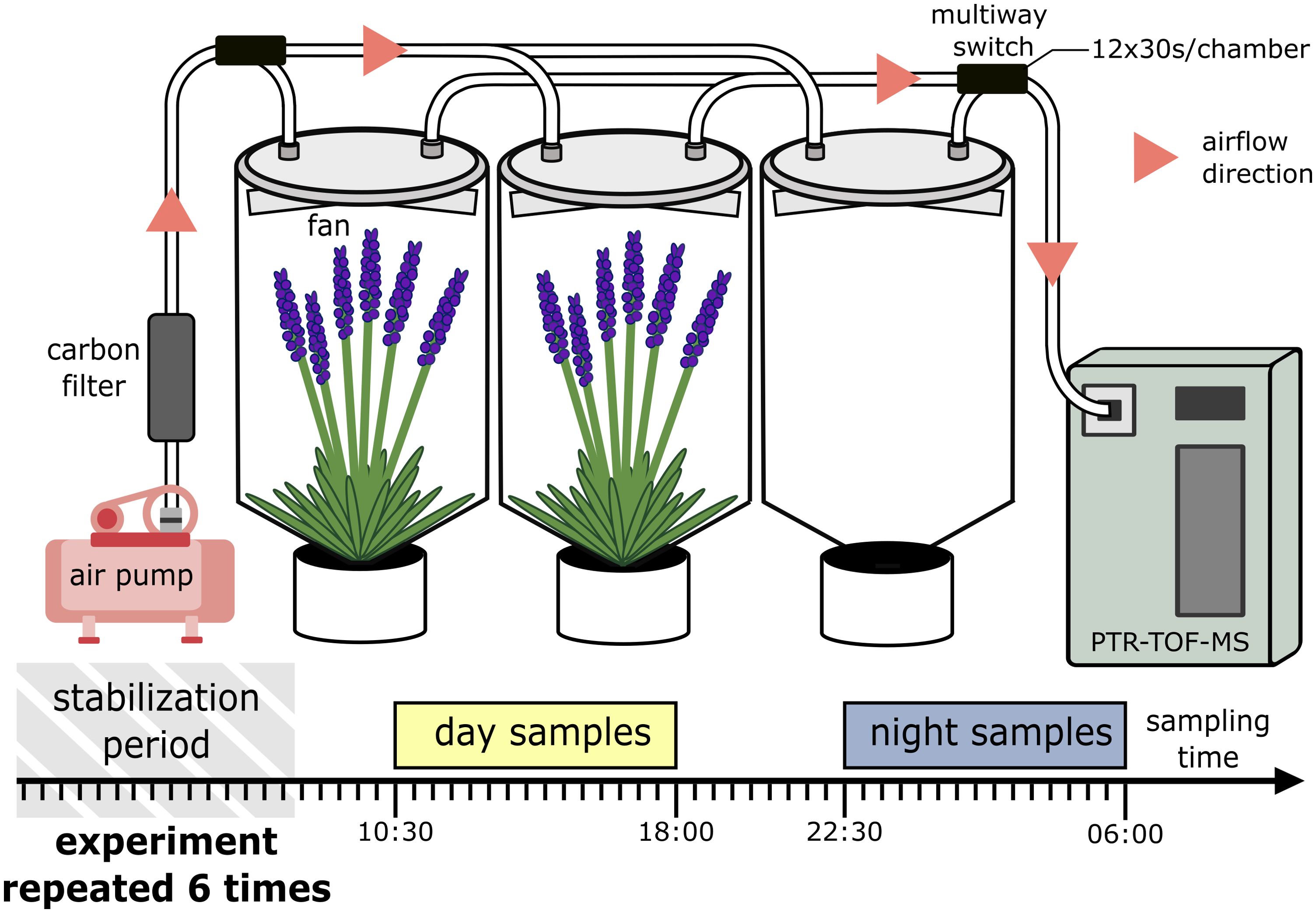
Figure 1. Schematic diagram of the experimental dynamic chamber system.
The raw data files created by the PTR-TOF-MS are in hierarchical data format (HDF), which is an open data format, characterized by a “.h5” extension. The raw data importation was done using the function named “import.h5()” from the provoc R package (Huguenin, 2022). This function uses different arguments to optimize the data resolution: a baseline correction argument that corrects the detector fluctuations and reduces the offsets in the m/z values, an argument that adjusts the peak size width, and the signal-to-noise ratio “SNR”. We conducted 12 sampling points per chamber, however, only the 6 last sampling points per chamber were included in the subsequent analysis. This decision was made due to possible cross-contamination of the chambers with the residual air from the previous chamber, resulting from the chamber-switching settings during sampling. When the data importation was done, the import.h5 function output gave a list of multiple objects. In the output list, a matrix automatically named “peaks” was created which represents the intensity values of m/z across multiple samples. In the output list, another matrix named “meta” was created that represents the metadata associated with each sample. Factors and factor levels were added to the matrix “meta”. The modified “meta” matrix was reintegrated into the output list. All the data importation and data optimization functions used in this publication were computed in the “provoc” R package (Huguenin, 2022).
Multivariate Curve Resolution (MCR) is the generic denomination referring to a family of methods employed to provide a chemically meaningful additive bilinear model of pure contributions solely from the information of an original data matrix (De Juan et al., 2014). For instance, consider a matrix M, where the rows represent the sampling time, and the columns represents the spectral information. Each row in the matrix contains a complete spectrum recorded at a specific time-point, and each column represents the evolution of a spectral component (such as wavelength, m/z, ppm …) over time. The MCR divides the whole matrix into several sub-spectra (Scomp) and their associated concentrations over time (Ccomp). Each Ccomp-Scomp combination is called a component. The particularity of the MCR and its primary distinction with the other bilinear models (like PCA), lies in its ability to non-orthogonally divide each spectral part of the matrix. This characteristic allows MCR to accurately reflect the natural properties of the chemical entities. Unlike other bilinear models, where each spectral part can only be considered in its totality, MCR divides each spectral part into several components. This method is ideally suited for data obtained by PTR-TOF-MS as each m/z gives a mixed contribution to the “pure” molecule spectra. For example, in PTR-TOF-MS fragmentation, the m/z 81 is characteristic of most monoterpenes fragmentation (unlike m/z 137 characteristic for monoterpenes with GC-MS fragmentation); the MCR analysis can divide the abundance of the m/z 81 of different monoterpenes as long as they have different co-varying patterns. However, MCR doesn’t have a default number of components, as a consequence of the “ambiguity of permutation” which implies that there is no priority order in the pure spectra and their associated concentration. The component number can go from 2 to infinite. Because of this aspect, setting the number of components during the analysis is necessary. The MCR method functions used in this publication are computed in the “provoc” R package (Huguenin, 2022).
Redundancy analysis as explained in Capblancq and Forester (2021) is a type of asymmetric canonical analysis that combines ordination and regression. First, a regression is performed on quantitative variables that are considered as response variables Y, on a set of explanatory variables X, thereby computing a new matrix of fitted values Y’. Then ordination is performed on Y’ with principal components analysis (PCA) for determining new synthetic composite variables (principal components or PC axes) which best capture the variance of the data. The RDA further partitions the total variance into constrained or factorial variance (proportion of variance explained by the explanatory variables of the model X on the dispersion of the response variables Y) and unconstrained or residual variance. It is usually represented in the form of a ratio between factorial variance (variance of Y explained by X) and residual variance (variance of Y not explained by X) and is termed as the Proportion of Constrained Inertia (PCI) (Oksanen, 2019). RDA is a non-parametric method suited for multivariate data. It models both multivariate response and multivariate explanatory variables and is thus particularly useful in the PTR-TOF-MS data analysis workflow to evaluate the optimal combination of normalization method and number of components (i.e. the combination that maximize the factorial explained variance. The RDA method functions used in this publication are computed in the “vegan” R package (Dixon, 2003).
To validate our workflow, we performed randomization of the data and compare the results of the RDA between randomized dataset and the real data. A randomized version of the intensity matrix “peaks” is created, where samples are randomly distributed between the factor levels (“sample()” function). For each dataset, we performed the MCR analysis to obtain the components. MCR are performed with 2 to 10 components on the output list containing the raw (or randomized) data intensity matrix “peaks” and the metadata matrix “meta”. Then, RDA analysis is performed on the Ccomp objects resulting from the MCR analysis. The RDA is performed on 2 factors including their possible interaction: plant/empty and day/night using the formula: “rda(data~factor1*factor2)”. This RDA measures how much variation in the m/z intensities of one component is explained by the explaining factors. ANOVA-like permutation tests anova(RDA) and MVA.anova(RDA) from package RVAideMemoire (Hervé and Hervé, 2023) are performed to test the significativeness of the model, the factors and their interaction.
The greater the factorial variance, the more meaningful the components are. This allows us to validate the use of MCR to decompose the data into biologically meaningful component according to our experimental factors. The workflow for this method validation is shown in Figure 2.
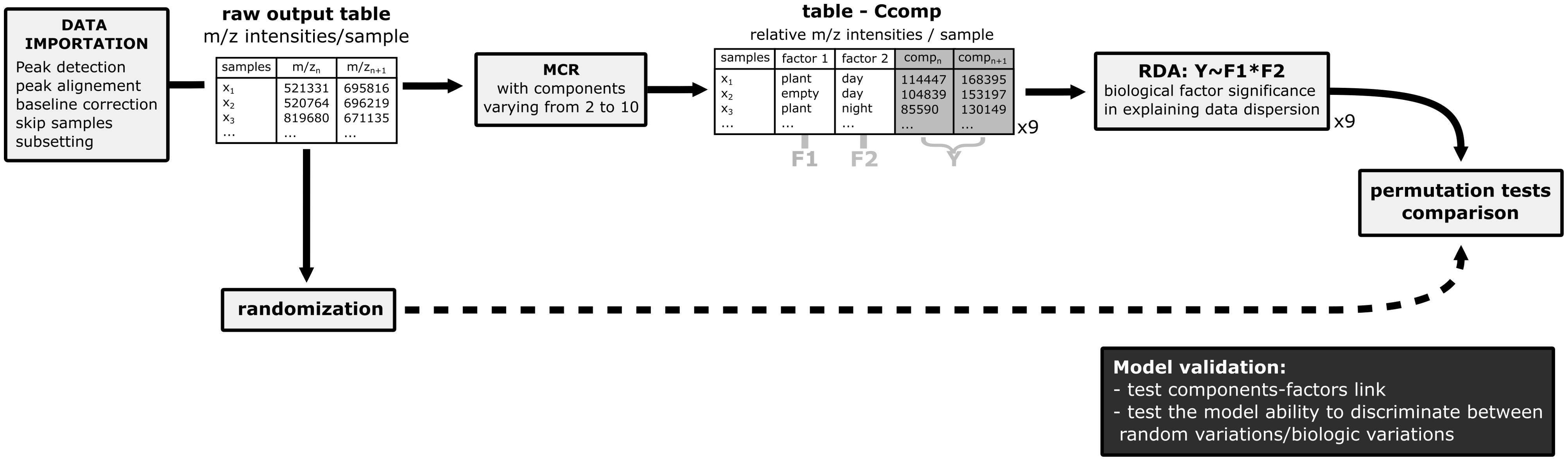
Figure 2. Schematic representation of the method validation workflow.
This process determines the parameters to be selected, which are specific to each data set.
Because of the natural inter-individual variability in BVOC emission, a normalization process must be applied to the raw data to allow comparison of replicates and minimize residual variance. It is important to standardize emissions between samples to reduce biological variability and better highlight the effect of explanatory factors. In our workflow of analysis, we have integrated several of the most widely used standardization methods. One of the most common relate the emissions to the dry weight of the sample. This method works if the dry mass is correlated with the surface area and the number of organs or cells producing and emitting VOCs. Another normalization method often used for metabolomic datasets is the normalization of each metabolic fingerprint to a specific “housekeeping” metabolite, like creatinine (Zacharias et al., 2018). For PTR-TOF-MS data a “housekeeping” m/z can be used instead of a “housekeeping” metabolite. Here, the m/z 59 was chosen because in PTR-TOF-MS fragmentation, the m/z 59 corresponds to acetone (Eerdekens et al., 2009). Acetone is known to be an oxidation product of isoprene (Jacob et al., 2002; Eerdekens et al., 2009), which emission is correlated with photosynthesis activity (Harley et al., 1996; Sharkey and Yeh, 2001). The quantity of the m/z 59 fragment reaches a plateau during the night, when there is no photosynthesis and when the emission is stable over time. This plateau defines a basic level that is specific to each sample. Therefore, a normalization factor is calculated using the ratio of the m/z 59 basic level of emission. This method allows to normalize emissions with the photosynthetic activity of the plant. Many mathematical normalization methods are also used for RMN (chemical data) or transcriptomic/genomic datasets. A selection of these methods is tested in our workflow and detailed in Table 2. In the importation output object, the intensity matrix “peaks” is normalized according to the different normalization methods and reintegrated into the output list.
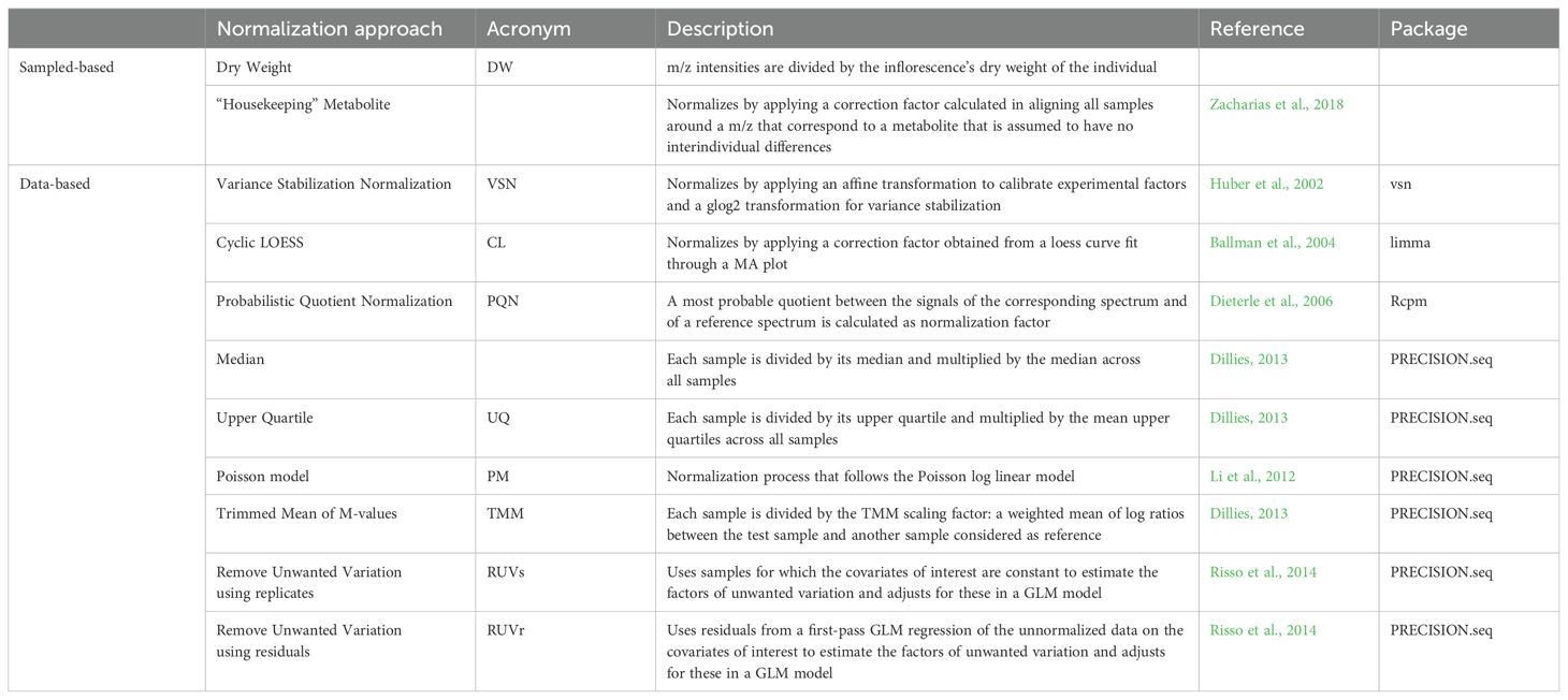
Table 2. Comparison table of different normalization methods used in this publication.
To determine the best normalization method and the most appropriate number of components. The normalization methods and the number of components were evaluated simultaneously. In that aim, the Ccomp data table should be re-organized so that the component number IDs becomes an explanatory factor (variable in column). This gives a new “modified Ccomp” matrix. For each normalization method, we tested the performance of the models with 2 to 10 components.
RDA are performed on each modified Ccomp matrix resulting from the MCR analysis. The model has only 1 factor: the component number ID (data~componentID). Thus, this RDA measures how much the variations in the m/z intensities behave in a similar way between day-replicates (low residual variance) and how well these different patterns of variation are discriminated between the different components (high factorial variance). The smaller the residual variance, the more closely the replicates are aligned with each other Figure 3, and therefore the better the normalization method is. At the same time, the greater the factorial variance is, the better the components explain the pattern of the data. Considering the number of components evaluation, in theory, we expect the Proportion of Constrained Inertia (PCI) to follow a hyperbole as a function of the number of components. This means that adding components helps to increase the explicative power of the factor up to a certain point where adding more components is not useful anymore. To determine which data point is the turning point in the hyperbole (called elbow or knee) the kneedle algorithm from the R package kneedle is used (Satopaa et al., 2011). In this study we chose to not go above 10 components because it was enough for the PCI hyperboles to reach a plateau, however the maximum number of components may need to be higher than 10, depending on the specificities of handled data. The schema for this case-by-case workflow is shown in Figure 4.
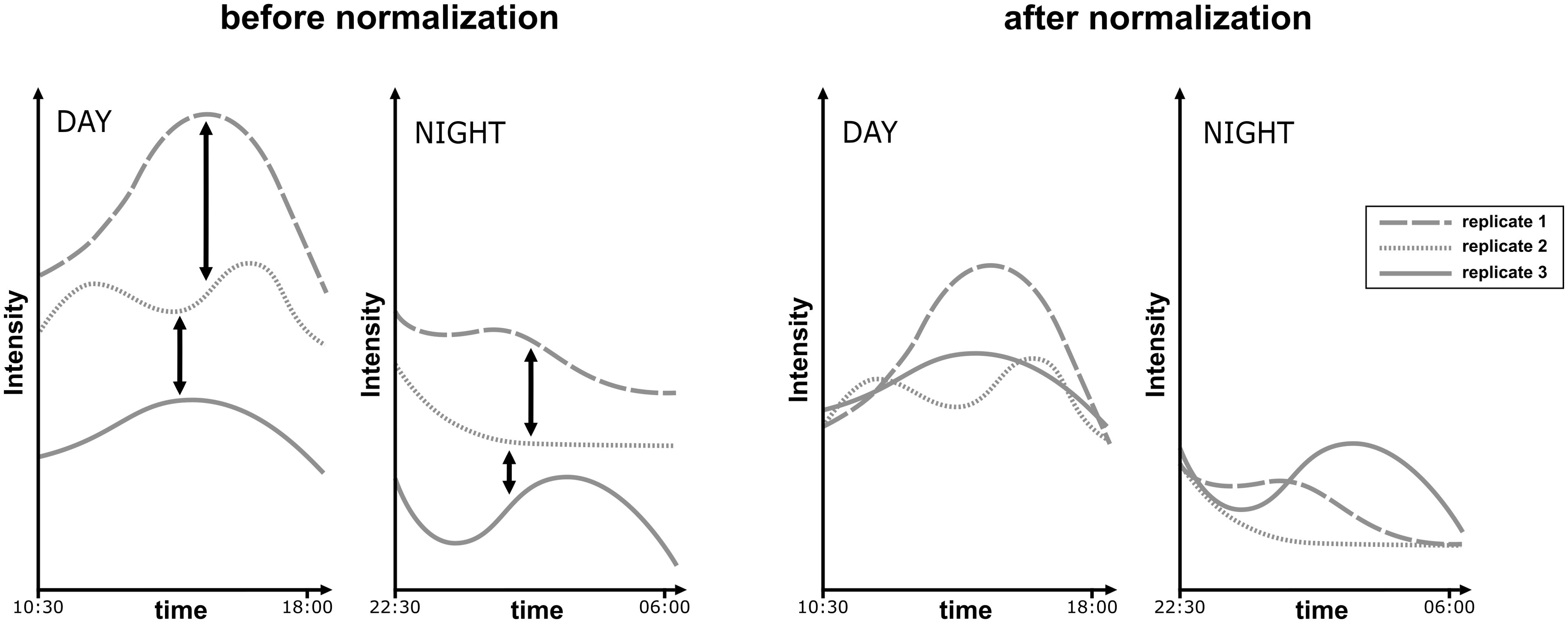
Figure 3. Schematic representation of replicates normalization. A necessary process to optimize factorial effect within components.
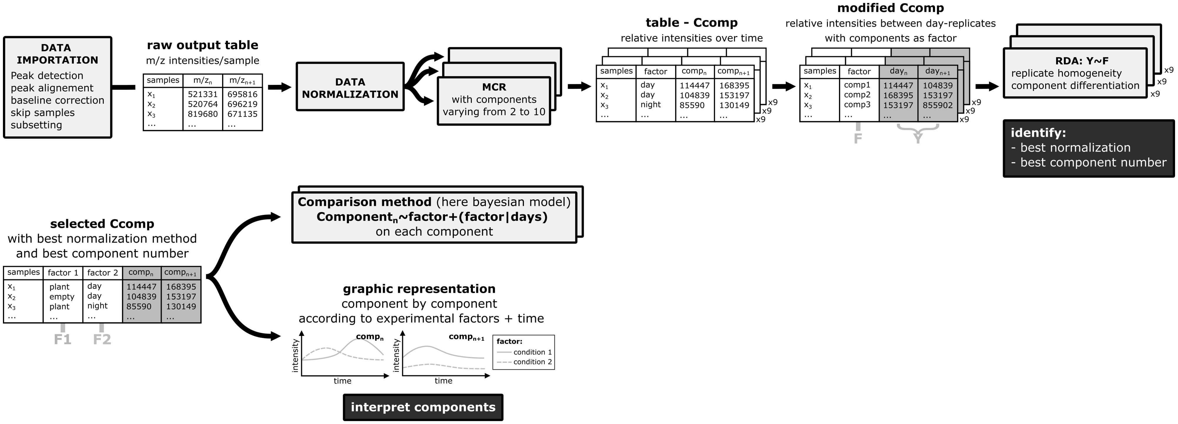
Figure 4. Schematic representation of the case-by-case workflow optimization process.
To identify the explanatory factor(s) for each component, we choose to use bayesian models, however other statistic methods such as a more classic mean-comparison ANOVA may be used, depending on the data specificities. Bayesian models allow to visualize more accurately the difference ranges between conditions. The Bayesian model, based on prior assumptions, calculates 95% probability intervals that correspond to the theoretical distribution of our values. We then compare the areas of overlap between the intervals for the different conditions to conclude on the significance of the differences. The Bayesian framework was carried out using the “brm()” function in the brms package (Bürkner, 2017). Both factors (day/night) and (plant/without plant) were combined in one (day/night/control) for a more meaningful graphical representation. The model used is a mixed model represented by the formula: “Componentn~factors + (factors|days)” which represent the m/z intensities of a component as a function of the experimental factors as fixed effects and considering the variability of experimental factors per day-replicate as a random effect. The model was computed as gaussian distribution, and the priors selected are a normal function with a mean and a standard deviation between 1e+05 and 1e+06 depending on each component intensities for the intercept and a normal function with a mean of 0 and a standard deviation between 1e+05 and 1e+06 depending on each component intensities for the beta-coefficient of conditions (b). The function was carried out with a warmup of 500, 2000 iterations and 3 MCMC (Markov chains Monte Carlo) chains. Bayesian models are only considered valid if MCMC chains reach their stationary distribution which is checked by convergence diagnostic. The convergence of the model was checked by plotting the variable “b_intercept”.
Faced with the difficulties of processing PTR-TOF-MS data, we have developed an analysis workflow based on 2 types of analysis: a MCR-based analysis to decompose the spectra into components that follow the same variation patterns, and a RDA-based analysis to assess the quality of the MCR in defining components linked to the factors. To evaluate the efficiency of the MCR method, we compared the results of MCR ran on a randomized dataset and those of MCR obtained from the raw data.
When analyzing the results of MCR analysis on the raw data, from 2 to 10 components, the RDA model demonstrate significance, indicating that the model’s factors are judicious and capture a significant share of Y variance. When we look at the significance of the explanatory factors, both the day/night effect and the presence of plant (plant/empty) have a significant effect (< 0.001) for all models (2 to 10 components) tested. In the case of the randomized data, all the p-values are > 0.05. This indicates that MCR analysis produce biologically meaningful components on the raw data compared to random data and can discriminate between real biological information and factors that are merely random and not linked to biological differences between the conditions. Moreover, the Proportions of Constrained Inertia PCIs for the raw matrix are around 0.6 whereas for the randomized matrix they are close to insignificant (<0.005) which means that the factors day/night and plant/empty explain a good part of the variation of the data inside each component when compared to chance. All RDA model statistical test outputs are shown in Supplementary Tables.
Cross-optimization of normalization method selection and determination of optimal number of components was performed, all resulting curves are represented in Figure 5. As expected, most of the curves follow a hyperbole except VSN, CL and RUVs. Furthermore, these methods give lower PCI than the non-normalized data indicating that they are not suited to normalize this dataset. The m/z59, TMM, PQN, PM, UQ, median and RUVr methods give higher PCI than the non-normalized data which means their normalization process helps RDA to increase the percentage of explanatory variance. Indeed, choosing the best normalization method may increase by a factor of 8 the factorial variance of the components explained by the factors (PCI=0.05 for VSN and 0.4 for RUVr). The highest PCI is found for the data normalized by RUVr method which is therefore selected for the following analyses. The kneedle algorithm indicates that the PCI increases less significantly after 5 components for the RUVr normalized data. The best optimization for this experimental dataset is a MCR with 5 components using a RUVr normalized dataset.
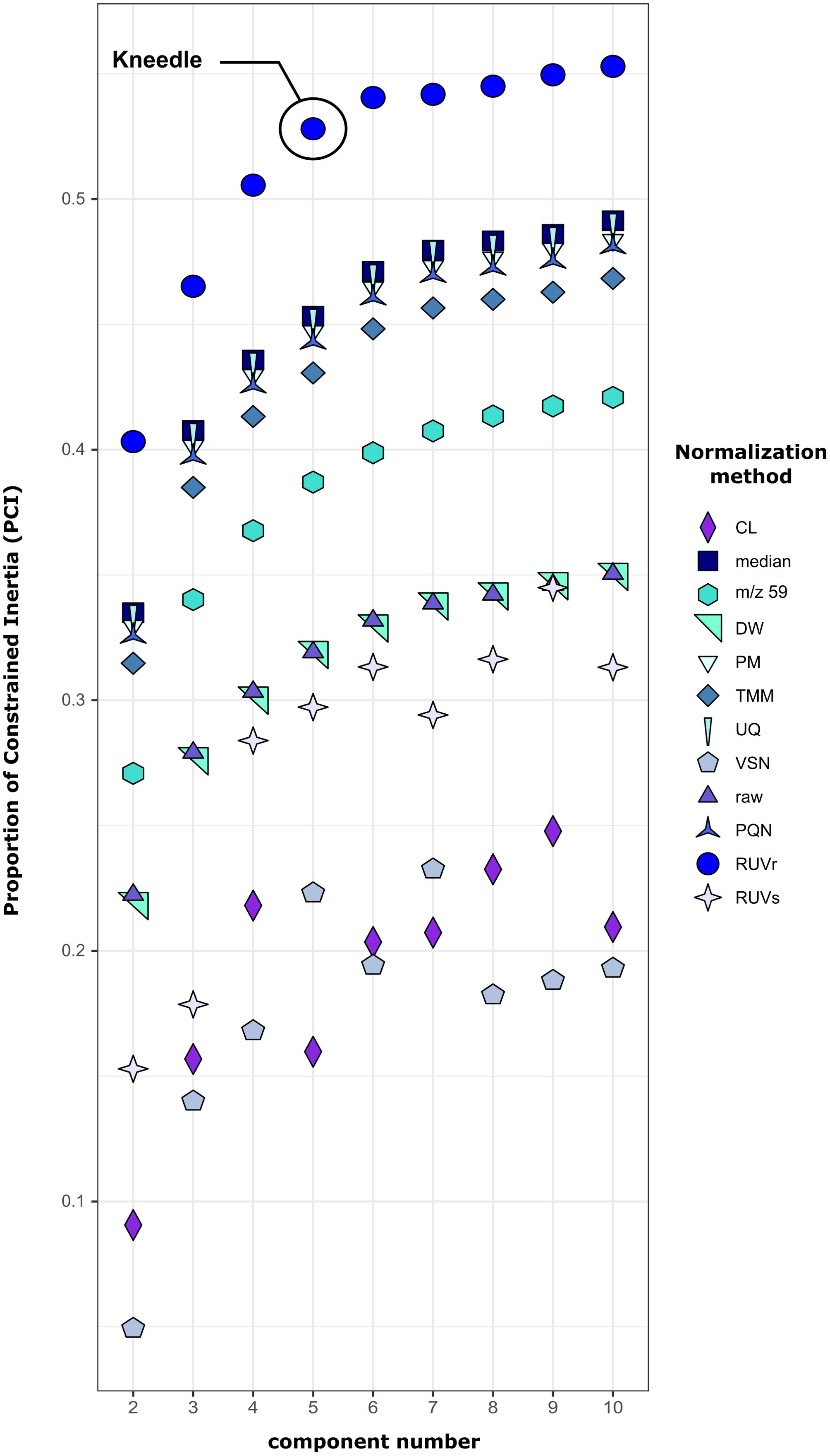
Figure 5. Redundancy analysis’s inertia proportion constrained with component number ID as explanatory factor depending on component number for all the normalization methods (detailed information can be found in Table 2).
The intensities associated with each component of the “Ccomp” table were aligned along the 8 hours sampling period for the day and night sampling. Start of sampling is then marked as zero relative hours for both sampling. The LOESS regression layout (LOcally Estimated Scatterplot Smoothing) is chosen to visualize the evolution of these concentrations according to time (Figure 6). Using Bayesian models, the predicted fitted values with 95% probability interval for each modality of the factor and each component are represented in Figure 7. Components 1 and 5 display no significant difference between the conditions as the 95% probability credible intervals overlap. Only the concentration of VOCs emitted during daytime in Component 1 and the concentration of VOCs in the empty chamber display marginal differences compared to the other condition: >85% of posterior distribution is positive (different and superior) compared the other conditions in both components. These components represent m/z belonging to the background noise of the global spectrum and hence cannot be associated with any explaining factors. Component 4 displays a higher intensity in the empty chamber in comparison to the chambers containing the plants (2.2e+05, 95% CI[1.3e+05, 2.4e+05]) with 100% of posterior distribution positive compared to the other conditions. This component visually doesn’t show variation over time, suggesting that it may correspond to the m/z mainly present in the ambient air of the greenhouse. The last 2 components display 2 different patterns of BVOCS over time. Component 2 shows a higher concentration of VOCs emitted during daytime (3e+06, 95% CI[7.8e+05, 3.9e+06]) with 99% of posterior distribution positive compared to VOCs emitted during nighttime. Both night and day distribution are different to control (100% of posterior distribution positive). Concentration of VOCs emitted during daytime also visually display gradual increase peaking after 6 hours of sampling i.e. at 4:30 pm. Component 3 shows a higher concentration of VOCs emitted during nighttime (9e+04, 95% CI[4e+04, 1.3e+05]) with 100% of posterior distribution positive compared to VOCs emitted during daytime. Here daytime and control distribution display no significant difference between the conditions as the 95% probability credible intervals overlap.
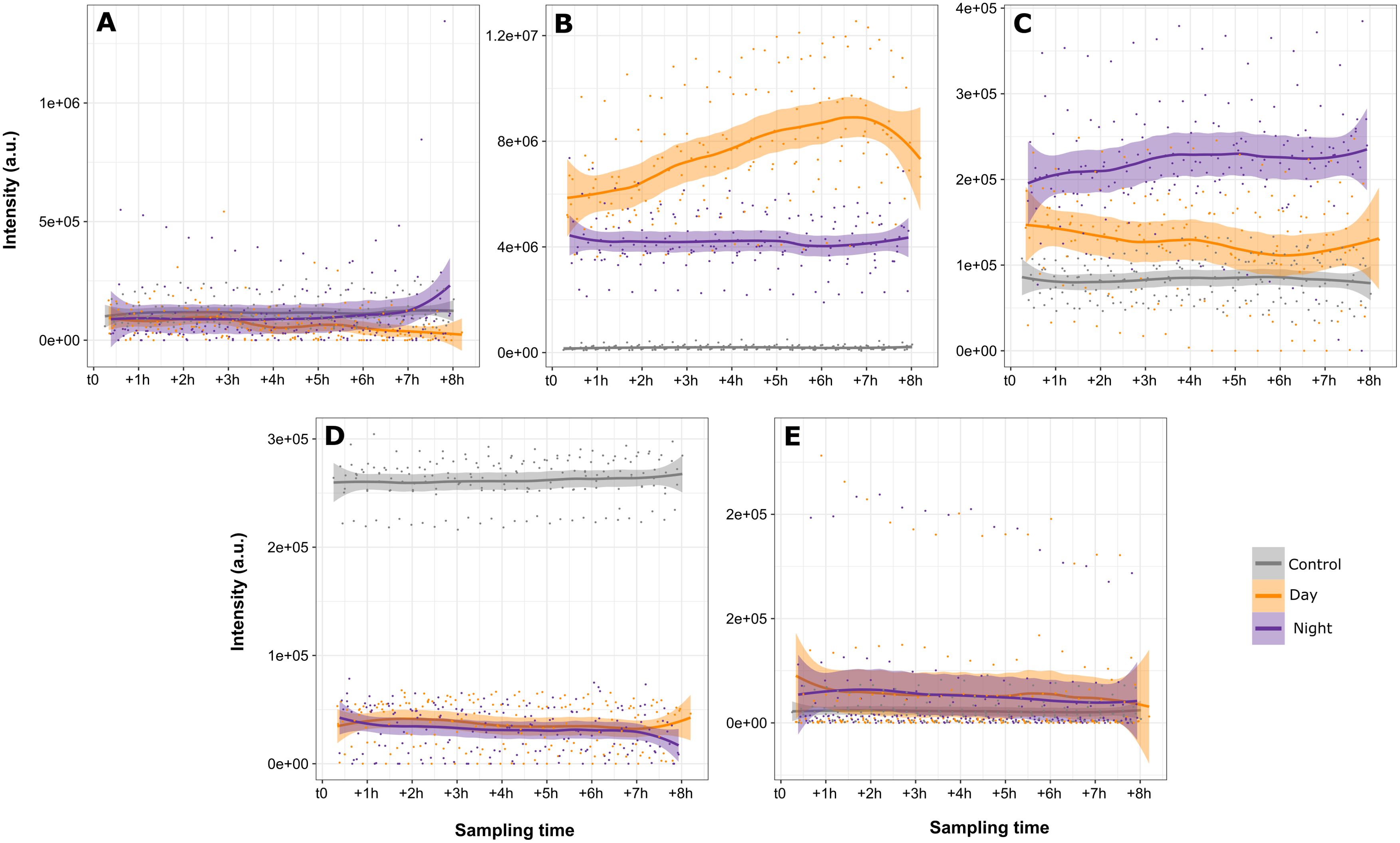
Figure 6. Visual representation with LOESS regression layout for each component. Variations in intensity of the m/z sum over 8 hours of sampling for each condition (control, day and night). Component 1 (A), component 2 (B), component 3 (C), component 4 (D) and component 5 (E).
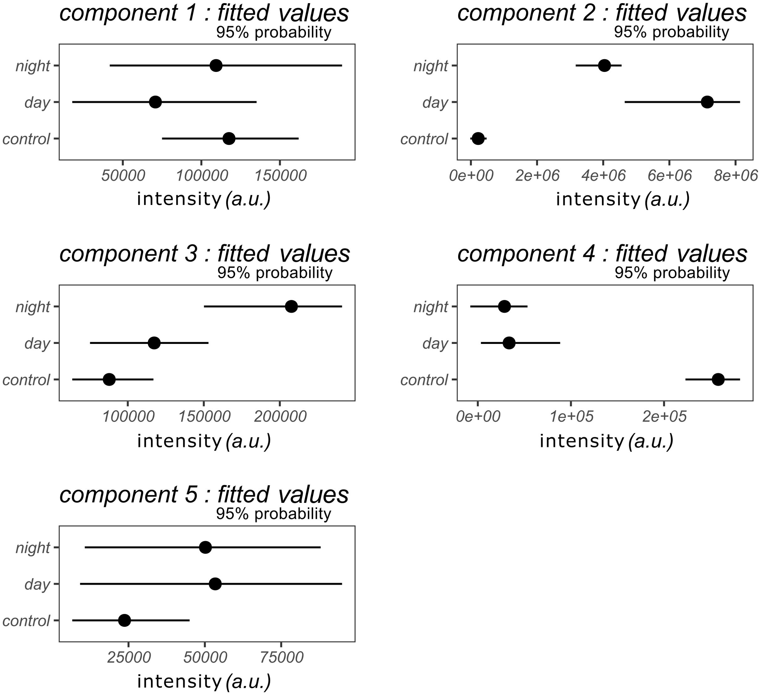
Figure 7. Graphical representation of the model fitted values for each condition (night, day and control) with credible 95% probability intervals for each component.
PTR-TOF-MS is an emerging technique in chemical ecology for temporal and «real-time» tracking VOC emission. Some studies using this technique for chemical ecology purposes are already published (Bracho-Nunez et al., 2011; Marotz-Clausen et al., 2018; Yáñez-Serrano et al., 2021), however the data analysis workflows are not always clearly detailed. Additionally, analyses are often focused on single m/z time tracking and not suited for complex VOC mixture sampling.
In this work, we have developed a generalizable and inter-operable data analysis workflow that facilitates handling the datasets with several replicates, explaining factors, and spectral similarities between compounds. This workflow features multiple innovative decision-making tools: an optimization process based on objective statistical analysis with a normalization selection method using multivariate redundancy analysis, while it is still mainly performed with visual or subjective criteria (Livera et al., 2015; Misra, 2020), or correlation coefficients (Wulff and Mitchell, 2018). We demonstrated that the Multivariate Curve Resolution method is able to divide a spectrum in biologically meaningful components related to the explained factors. With this method, a way to overcome the intrinsic “ambiguity of permutation” by selecting the optimal component number is proposed, also using multivariate redundancy analysis. The workflow proposed in this publication improves PTR-TOF-MS data interpretation. It can be used as an all-in-hand guide to handle PTR-TOF-MS data analysis more easily with different evaluation tests throughout the workflow to help choose the different parameters and adapt the method to the specificities of the data. Both normalization and component number selection are performed simultaneously.
There is one main difficulty to promote the use of PTR-TOF-MS in chemical ecology i.e. the individual compound identification. The current study addresses this issue by proposing a new way to decompose the data, therefore reducing the uncertainty. It achieves this by dividing the whole data in smaller batch of compounds that exhibit similar patterns and by dividing the total mass spectrum into several sub-mass spectra associated with these batch of compounds. To identify the compounds individually, standards fragmentation spectra are still needed as there are no libraries available for this technique. Although mass spectra libraries for PTR-TOF-MS data do not exist yet, nonetheless some publications have utilized the m/z resulting from the fragmentation of common molecules as a reference to help with the identification (Lee et al., 2006; Maleknia et al., 2007; Yáñez-Serrano et al., 2021; Roslund et al., 2021). For now, the use of standard Headspace GC-MS sampling is still needed in parallel to identify single compounds that could fit to the variation patterns obtained by PTR-Tof-MS. Altogether, we advocate for the widespread use of multi-sampling approaches to precisely determine VOC emission variations in complex chemical profiles.
Moreover, the data-analysis workflow has some requirements, i.e. at least one experimental factor or condition with minimum 2 different levels needed for the evaluation of the components number, and the normalization methods. It also requires a non-continuous sampling with regular switching between replicates or conditions. Lastly, it also requires biological replicates for each condition to give accurate results, depending on how much inter-individual variation is found in the studied model.
PTR-TOF-MS is a helpful technique for long time sampling due to its automatization, especially if the experiment requires a day and night sampling for several days in a row. The method is also non-destructive and allows to keep the studied organisms in good conditions to analyze their emission over a long period of time. The high accuracy of PTR-TOF-MS sampling associated with the data analysis workflow proposed here holds potential for numerous applications in chemical ecology and metabolomics. Indeed, even if data annotation has to be further developed, the present method remains efficient to compare VOC’s patterns and is a promising approach for conducting in depth study of BVOC emissions from biological models with a large metabolome or with low emission quantities.
The original contributions presented in the study are included in the article/Supplementary Material. Further inquiries can be directed to the corresponding author/s.
MF: Conceptualization, Data curation, Methodology, Writing – original draft, Writing – review & editing, Formal Analysis, Investigation, Software, Visualization. JH: Data curation, Software, Supervision, Writing – review & editing. FJ: Supervision, Writing – review & editing. SM: Writing – review & editing, Supervision. MP: Conceptualization, Supervision, Writing – review & editing, Funding acquisition, Project administration. FN: Conceptualization, Data curation, Methodology, Supervision, Validation, Writing – review & editing, Funding acquisition, Project administration.
The author(s) declare that financial support was received for the research and/or publication of this article. This work was partly funded by the Laboratoire d’Excellence Centre Méditerranéen Environnement et Biodiversité (LabEx CeMEB), the Montpellier Université d’Excellence (MUSE, ANR under the Investissements d’avenir program, reference ANR-16-IDEX-0006), the French National Research Program for Environmental and Occupational Health of ANSES (reference 2018/1/138), the program FEDER-FSE-IEJ Languedoc-Roussillon 2014-2020 n°2014FR16MOOP006, the AAP (Mobilité Formation) 2022 grant, provided by FR BioEEnVis.
The authors declare that the research was conducted in the absence of any commercial or financial relationships that could be construed as a potential conflict of interest.
The author(s) declare that no Generative AI was used in the creation of this manuscript.
All claims expressed in this article are solely those of the authors and do not necessarily represent those of their affiliated organizations, or those of the publisher, the editors and the reviewers. Any product that may be evaluated in this article, or claim that may be made by its manufacturer, is not guaranteed or endorsed by the publisher.
The Supplementary Material for this article can be found online at: https://www.frontiersin.org/articles/10.3389/fevo.2025.1536032/full#supplementary-material
Abbas F., Ke Y., Yu R., Yue Y., Amanullah S., Jahangir M. M., et al. (2017). Volatile terpenoids: multiple functions, biosynthesis, modulation and manipulation by genetic engineering. Planta 246, 803–816. doi: 10.1007/s00425-017-2749-x
Aharoni A., Giri A. P., Deuerlein S., Griepink F., De Kogel W.-J., Verstappen F. W. A., et al. (2003). Terpenoid metabolism in wild-type and transgenic arabidopsis plants. Plant Cell. 15, 2866–2884. doi: 10.1105/tpc.016253
Baghi R., Helmig D., Guenther A., Duhl T., Daly R. (2012). Contribution of flowering trees to urban atmospheric biogenic volatile organic compound emissions. Biogeosciences 9, 3777–3785. doi: 10.5194/bg-9-3777-2012
Ballman K. V., Grill D. E., Oberg A. L., Therneau T. M. (2004). Faster cyclic loess: normalizing RNA arrays via linear models. Bioinformatics 20, 2778–2786. doi: 10.1093/bioinformatics/bth327
Bracho-Nunez A., Welter S., Staudt M., Kesselmeier J. (2011). Plant-specific volatile organic compound emission rates from young and mature leaves of Mediterranean vegetation. J. Geophys Res. 116, D16304. doi: 10.1029/2010JD015521
Brilli F., Ruuskanen T. M., Schnitzhofer R., Müller M., Breitenlechner M., Bittner V., et al. (2011). Detection of plant volatiles after leaf wounding and darkening by proton transfer reaction “Time-of-flight” Mass spectrometry (PTR-TOF). PloS One 6, e20419. doi: 10.1371/journal.pone.0020419
Bürkner P.-C. (2017). brms: an R package for bayesian multilevel models using stan. J. Stat. Soft. 80 (1), 1–28. doi: 10.18637/jss.v080.i01
Cáceres L. A., Lakshminarayan S., Yeung K. K.-C., McGarvey B. D., Hannoufa A., Sumarah M. W., et al. (2016). Repellent and attractive effects of α-, β-, and dihydro-β- ionone to generalist and specialist herbivores. J. Chem. Ecol. 42, 107–117. doi: 10.1007/s10886-016-0669-z
Capblancq T., Forester B. R. (2021). Redundancy analysis: A Swiss Army Knife for landscape genomics. Methods Ecol. Evol. 12, 2298–2309. doi: 10.1111/2041-210X.13722
Cappellin L., Aprea E., Granitto P., Romano A., Gasperi F., Biasioli F. (2013). Multiclass methods in the analysis of metabolomic datasets: The example of raspberry cultivar volatile compounds detected by GC–MS and PTR-MS. Food Res. Int. 54, 1313–1320. doi: 10.1016/j.foodres.2013.02.004
Cappellin L., Aprea E., Granitto P., Wehrens R., Soukoulis C., Viola R., et al. (2012). Linking GC-MS and PTR-TOF-MS fingerprints of food samples. Chemometrics Intelligent Lab. Systems 118, 301–307. doi: 10.1016/j.chemolab.2012.05.008
Curvers J., Th N., Cramers C., Rijks J. (1984). Possibilities and limitations of dynamic headspace sampling as a pre-concentration technique for trace analysis of organics by capillary gas chromatography. J. Chromatogr. A. 289, 171–182. doi: 10.1016/S0021-9673(00)95086-6
De Juan A., Jaumot J., Tauler R. (2014). Multivariate curve resolution (MCR). Solving mixture Anal. problem Anal. Methods 6, 4964–4976. doi: 10.1039/C4AY00571F
Deng C., Zhang X., Zhu W., Qian J. (2004). Investigation of tomato plant defence response to tobacco mosaic virus by determination of methyl salicylate with SPME-capillary GC-MS. Chromatographia 59, 263–268. doi: 10.1365/s10337-003-0144-1
Dieterle F., Ross A., Schlotterbeck G., Senn H. (2006). Probabilistic quotient normalization as robust method to account for dilution of complex biological mixtures. Application in 1 H NMR metabonomics. Anal. Chem. 78, 4281–4290. doi: 10.1021/ac051632c
Dillies M.-A., Rau A., Aubert J., Hennequet-Antier C., Jeanmougin M., Servant N., et al. (2013). A comprehensive evaluation of normalization methods for Illumina high-throughput RNA sequencing data analysis. Briefings Bioinf. 14, 671–683. doi: 10.1093/bib/bbs046
Dixon P. (2003). VEGAN, a package of R functions for community ecology. J. Vegetation Sci. 14, 927–930. doi: 10.1111/j.1654-1103.2003.tb02228.x
Dubuisson C., Nicolè F., Buatois B., Hossaert-McKey M., Proffit M. (2022). Tropospheric ozone alters the chemical signal emitted by an emblematic plant of the mediterranean region: the true lavender (Lavandula angustifolia mill.). Front. Ecol. Evol. 10, 795588. doi: 10.3389/fevo.2022.795588
Dudareva N., Klempien A., Muhlemann J. K., Kaplan I. (2013). Biosynthesis, function and metabolic engineering of plant volatile organic compounds. New Phytol. 198, 16–32. doi: 10.1111/nph.2013.198.issue-1
Durenne B., Blondel A., Druart P., Fauconnier M.-L. (2018). A laboratory high-throughput glass chamber using dynamic headspace TD-GC/MS method for the analysis of whole Brassica napus L. plantlet volatiles under cadmium-related abiotic stress. Phytochemical Analysis 29, 463–471. doi: 10.1002/pca.v29.5
Eerdekens G., Ganzeveld L., de Arellano J. V.-G., Harder H., Kubistin D., Martinez M., et al. (2009). Flux estimates of isoprene, methanol and acetone from airborne PTR-MS measurements over the tropical rainforest during the GABRIEL 2005 campaign. Atmos Chem. Phys. 9, 4207–4227. doi: 10.5194/acp-9-4207-2009
Ennis C. J., Reynolds J. C., Keely B. J., Carpenter L. J. (2005). A hollow cathode proton transfer reaction time of flight mass spectrometer. Int. J. Mass Spectrometry 247, 72–80. doi: 10.1016/j.ijms.2005.09.008
Giacomuzzi V., Cappellin L., Khomenko I., Biasioli F., Schütz S., Tasin M., et al. (2016). Emission of volatile compounds from apple plants infested with pandemis heparana larvae, antennal response of conspecific adults, and preliminary field trial. J. Chem. Ecol. 42, 1265–1280. doi: 10.1007/s10886-016-0794-8
Greenberg J. P., Asensio D., Turnipseed A., Guenther A. B., Karl T., Gochis D. (2012). Contribution of leaf and needle litter to whole ecosystem BVOC fluxes. Atmospheric Environment 59, 302–311. doi: 10.1016/j.atmosenv.2012.04.038
Han C., Liu R., Luo H., Li G., Ma S., Chen J., et al. (2019). Pollution profiles of volatile organic compounds from different urban functional areas in Guangzhou China based on GC/MS and PTR-TOF-MS: Atmospheric environmental implications. Atmospheric Environment 214, 116843. doi: 10.1016/j.atmosenv.2019.116843
Hare J. D. (2011). Ecological role of volatiles produced by plants in response to damage by herbivorous insects. Annu. Rev. Entomol. 56, 161–180. doi: 10.1146/annurev-ento-120709-144753
Harley P., Guenther A., Zimmerman P. (1996). Effects of light, temperature and canopy position on net photosynthesis and isoprene emission from sweetgum (Liquidambar styraciflua) leaves. Tree Physiol. 16, 25–32. doi: 10.1093/treephys/16.1-2.25
Heiden A. C., Hoffmann T., Kahl J., Kley D., Klockow D., Langebartels C., et al. (1999). Emission of volatile organic compounds from ozone-exposed plants. Ecol. Appl. 9(4), 1160–1167. doi: 10.1890/1051-0761(1999)009[1160:EOVOCF]2.0.CO;2
Hervé M., Hervé M. M. (2023). Package ‘rvAideMemoire’. Available online at: https://cran.r-project.org/web/packages/RVAideMemoire/ (Accessed August 01, 2023).
Huang X.-F., Zhang B., Xia S.-Y., Han Y., Wang C., Yu G.-H., et al. (2020). Sources of oxygenated volatile organic compounds (OVOCs) in urban atmospheres in North and South China. Environ. Pollution 261, 114152. doi: 10.1016/j.envpol.2020.114152
Huber W., Von Heydebreck A., Sültmann H., Poustka A., Vingron M. (2002). Variance stabilization applied to microarray data calibration and to the quantification of differential expression. Bioinformatics 18, S96–S104. doi: 10.1093/bioinformatics/18.suppl_1.S96
Huguenin J. (2022). UMR 5175 CEFE, CNRS, University of Montpellier. provoc: analyze data of VOC by PTR-ToF-MS Vocus. doi: 10.5281/zenodo.6642830
Jacob D. J., Field B. D., Jin E. M., Bey I., Li Q., Logan J. A., et al. (2002). Atmospheric budget of acetone. J. Geophys Res. 107, ACH 5–1-ACH 5-17. doi: 10.1029/2001JD000694
Kaser L., Karl T., Guenther A., Graus M., Schnitzhofer R., Turnipseed A., et al. (2013). Undisturbed and disturbed above canopy ponderosa pine emissions: PTR-TOF-MS measurements and MEGAN 2.1 model results. Atmos Chem. Phys. 13, 11935–11947. doi: 10.5194/acp-13-11935-2013
Kesselmeier J., Staudt M. (1999). Biogenic volatile organic compounds (VOC): an overview on emission, physiology and ecology. J. Atmospheric Chem. 33, 23–88. doi: 10.1023/A:1006127516791
Kim S., Karl T., Guenther A., Tyndall G., Orlando J., Harley P., et al. (2010). Emissions and ambient distributions of Biogenic Volatile Organic Compounds (BVOC) in a ponderosa pine ecosystem: interpretation of PTR-MS mass spectra. Atmos Chem. Phys. 10, 1759–1771. doi: 10.5194/acp-10-1759-2010
Kolari P., Bäck J., Taipale R., Ruuskanen T. M., Kajos M. K., Rinne J., et al. (2012). Evaluation of accuracy in measurements of VOC emissions with dynamic chamber system. Atmospheric Environment 62, 344–351. doi: 10.1016/j.atmosenv.2012.08.054
Lee A., Goldstein A. H., Kroll J. H., Ng N. L., Varutbangkul V., Flagan R. C., et al. (2006). Gas-phase products and secondary aerosol yields from the photooxidation of 16 different terpenes. J. Geophys Res. 111, D17305. doi: 10.1029/2006JD007050
Li M., Cappellin L., Xu J., Biasioli F., Varotto C. (2020). High-throughput screening for in planta characterization of VOC biosynthetic genes by PTR-ToF-MS. J. Plant Res. 133, 123–131. doi: 10.1007/s10265-019-01149-z
Li J., Witten D. M., Johnstone I. M., Tibshirani R. (2012). Normalization, testing, and false discovery rate estimation for RNA-sequencing data. Biostatistics 13, 523–538. doi: 10.1093/biostatistics/kxr031
Lindinger W., Jordan A. (1998). Proton-transfer-reaction mass spectrometry (PTR–MS): on-line monitoring of volatile organic compounds at pptv levels. Chem. Soc. Rev. 27, 347. doi: 10.1039/a827347z
Lindinger C., Pollien P., Ali S., Yeretzian C., Blank I., Märk T. (2005). Unambiguous identification of volatile organic compounds by proton-transfer reaction mass spectrometry coupled with GC/MS. Anal. Chem. 77, 4117–4124. doi: 10.1021/ac0501240
Livera A. M. D., Sysi-Aho M., Jacob L., Gagnon-Bartsch J. A., Castillo S., Simpson J. A., et al. (2015). Statistical methods for handling unwanted variation in metabolomics data. Anal. Chem. 87, 3606–3615. doi: 10.1021/ac502439y
Maleknia S. D., Bell T. L., Adams M. A. (2007). PTR-MS analysis of reference and plant-emitted volatile organic compounds. Int. J. Mass Spectrometry 262, 203–210. doi: 10.1016/j.ijms.2006.11.010
Marotz-Clausen G., Jürschik S., Fuchs R., Schäffler I., Sulzer P., Gibernau M., et al. (2018). Incomplete synchrony of inflorescence scent and temperature patterns in Arum maculatum L.(Araceae). Phytochemistry 154, 77–84. doi: 10.1016/j.phytochem.2018.07.001
Misra B. B. (2020). Data normalization strategies in metabolomics: Current challenges, approaches, and tools. Eur. J. Mass Spectrom (Chichester) 26, 165–174. doi: 10.1177/1469066720918446
Mookherjee B. D., Trenkle R. W., Wilson R. A. (1989). Live vs. Dead. Part II. A comparative analysis of the headspace volatiles of some important fragrance and flavor raw materials. J. Essential Oil Res. 1, 85–90. doi: 10.1080/10412905.1989.9697755
Mozaffar A., Schoon N., Bachy A., Digrado A., Heinesch B., Aubinet M., et al. (2018). Biogenic volatile organic compound emissions from senescent maize leaves and a comparison with other leaf developmental stages. Atmospheric Environment 176, 71–81. doi: 10.1016/j.atmosenv.2017.12.020
Oksanen J. (2019). Vegan: an introduction to ordination. Available online at: https://CRAN.R-project.org/package=vegan.
Peñuelas J., Staudt M. (2010). BVOCs and global change. Trends Plant Sci. 15, 133–144. doi: 10.1016/j.tplants.2009.12.005
Perera R. M. M., Marriott P. J., Galbally I. E. (2002). Headspace solid-phase microextraction—comprehensive two-dimensional gas chromatography of wound induced plant volatile organic compound emissions. Analyst 127, 1601–1607. doi: 10.1039/B208577A
Proffit M., Bessière J.-M., Schatz B., Hossaert-McKey M. (2018). Can fine-scale post-pollination variation of fig volatile compounds explain some steps of the temporal succession of fig wasps associated with Ficus racemosa? Acta Oecologica 90, 81–90. doi: 10.1016/j.actao.2017.08.009
Proffit M., Schatz B., Bessiere J.-M., Cheri C., Soler C., Hossaert-McKey M. (2008). Signalling receptivity: Comparison of the emission of volatile compounds by figs of Ficus hispida before, during and after the phase of receptivity to pollinators. Symbiosis (Rehovot), 45 (1), 15.
Risso D., Ngai J., Speed T. P., Dudoit S. (2014). Normalization of RNA-seq data using factor analysis of control genes or samples. Nat. Biotechnol. 32, 896–902. doi: 10.1038/nbt.2931
Roquencourt C., Grassin-Delyle S., Thévenot E. A. (2022). ptairMS: real-time processing and analysis of PTR-TOF-MS data for biomarker discovery in exhaled breath.Vitek O, editor. Bioinformatics 38, 1930–1937. doi: 10.1093/bioinformatics/btac031
Roslund K., Lehto M., Pussinen P., Hartonen K., Groop P.-H., Halonen L., et al. (2021). Identifying volatile in vitro biomarkers for oral bacteria with proton-transfer-reaction mass spectrometry and gas chromatography–mass spectrometry. Sci. Rep. 11, 16897. doi: 10.1038/s41598-021-96287-7
Satopaa V., Albrecht J., Irwin D., Raghavan B. (2011). “Finding a “Kneedle” in a haystack: detecting knee points in system behavior,” in 2011 31st International Conference on Distributed Computing Systems Workshops. 166–171 (Minneapolis, MN, USA: IEEE). doi: 10.1109/ICDCSW.2011.20
Schueuermann C., Bremer P., Silcock P. (2017). PTR-MS volatile profiling of Pinot Noir wines for the investigation of differences based on vineyard site: PTR-MS volatile profiling of Pinot Noir wines. J. Mass Spectrom 52, 625–631. doi: 10.1002/jms.v52.9
Sharkey T. D., Yeh S. (2001). Isoprene emission from plants. Annu. Rev. Plant Physiol. Plant Mol. Biol. 52, 407–436. doi: 10.1146/annurev.arplant.52.1.407
Taiti C., Costa C., Guidi Nissim W., Bibbiani S., Azzarello E., Masi E., et al. (2017). Assessing VOC emission by different wood cores using the PTR-ToF-MS technology. Wood Sci. Technol. 51, 273–295. doi: 10.1007/s00226-016-0866-5
Tanimoto H., Aoki N., Inomata S., Hirokawa J., Sadanaga Y. (2007). Development of a PTR-TOFMS instrument for real-time measurements of volatile organic compounds in air. Int. J. Mass Spectrometry 263, 1–11. doi: 10.1016/j.ijms.2007.01.009
Tholl D., Weinhold A., Röse U. S. R. (2020). “Practical approaches to plant volatile collection and analysis,” in Biology of Plant Volatiles. Eds. Pichersky E., Dudareva N. (CRC Press, Boca Raton, FL).
Wulff J. E., Mitchell M. W. (2018). A comparison of various normalization methods for LC/MS metabolomics data. ABB 09, 339–351. doi: 10.4236/abb.2018.98022
Yáñez-Serrano A. M., Bach A., Bartolomé-Català D., Matthaios V., Seco R., Llusià J., et al. (2021). Dynamics of volatile organic compounds in a western Mediterranean oak forest. Atmospheric Environment 257, 118447. doi: 10.1016/j.atmosenv.2021.118447
Yáñez-Serrano A. M., Nölscher A. C., Williams J., Wolff S., Alves E., Martins G. A., et al. (2015). Diel and seasonal changes of biogenic volatile organic compounds within and above an Amazonian rainforest. Atmos Chem. Phys. 15, 3359–3378. doi: 10.5194/acp-15-3359-2015
Yang Z., Baldermann S., Watanabe N. (2013). Recent studies of the volatile compounds in tea. Food Res. Int. 53, 585–599. doi: 10.1016/j.foodres.2013.02.011
Zacharias H., Altenbuchinger M., Gronwald W. (2018). Statistical analysis of NMR metabolic fingerprints: established methods and recent advances. Metabolites 8, 47. doi: 10.3390/metabo8030047
Keywords: PTR-ToF-MS (proton transfer reaction time-of-flight mass spectrometry), chemical ecology, data analysis workflow, Lavandula angustifolia, VOC emission
Citation: Fontez M, Huguenin J, Jullien F, Moja S, Proffit M and Nicole F (2025) A practical workflow to facilitate analysis of the emission dynamics of non-target BVOCs in terrestrial ecosystems by PTR-TOF-MS. Front. Ecol. Evol. 13:1536032. doi: 10.3389/fevo.2025.1536032
Received: 28 November 2024; Accepted: 17 March 2025;
Published: 11 April 2025.
Edited by:
Juan Manuel Alba, The Institute for Mediterranean and Subtropical Horticulture “La Mayora” (IHSM-UMA-CSIC), SpainReviewed by:
Stefan Dötterl, University of Salzburg, AustriaCopyright © 2025 Fontez, Huguenin, Jullien, Moja, Proffit and Nicole. This is an open-access article distributed under the terms of the Creative Commons Attribution License (CC BY). The use, distribution or reproduction in other forums is permitted, provided the original author(s) and the copyright owner(s) are credited and that the original publication in this journal is cited, in accordance with accepted academic practice. No use, distribution or reproduction is permitted which does not comply with these terms.
*Correspondence: Mathias Fontez, bWF0aGlhcy5mb250ZXpAdW5pdi1zdC1ldGllbm5lLmZy
Disclaimer: All claims expressed in this article are solely those of the authors and do not necessarily represent those of their affiliated organizations, or those of the publisher, the editors and the reviewers. Any product that may be evaluated in this article or claim that may be made by its manufacturer is not guaranteed or endorsed by the publisher.
Research integrity at Frontiers
Learn more about the work of our research integrity team to safeguard the quality of each article we publish.