 Alexandra K. Schneider
 Mary C. Fabrizio
 Romuald N. Lipcius
- Virginia Institute of Marine Science, William & Mary, Gloucester Point, VA, United States
Global temperatures are rising across marine ecosystems in response to climate change. Marine and estuarine-dependent species including the blue crab, Callinectes sapidus, may adapt to warming temperatures phenologically, by shifting the seasonal timing of biological events, such as reproduction. In Chesapeake Bay, average water temperatures have risen by an average 0.02°C per year since the 1980s. Extension of the blue crab spawning season, through earlier onset and later conclusion, may augment annual brood production and alter the efficacy of management strategies. The duration of the potential spawning season from 1985 to 2019 was assessed using degree days, and the observed spawning season from 1995 to 2019 was assessed using the occurrence of ovigerous crabs from the Virginia Institute of Marine Science Trawl Survey in the James River and in the mainstem of lower Chesapeake Bay. Spawning degree days (SDD) and reproductive degree days (RDD) were defined using minimum temperatures of 19°C and 12°C, respectively. The mean duration of the potential spawning season increased by 25% in SDD and 10% in RDD between 1985 and 2019 in the James River and lower Chesapeake Bay, respectively. This progressive expansion of the potential spawning season was not, however, reflected in the observed spawning season. Rather, the onset, conclusion, and duration of the observed spawning season were variable over the time series. The observed month of onset was driven by RDD in spring, whereby spawning began earlier during warmer springs. The spawning conclusion date was driven by the onset of spawning, rather than Fall temperature, such that the duration of the observed spawning season and, therefore, annual brood production did not change over time. In Chesapeake Bay, the spawning stock is protected by a sanctuary that is closed to fishing from mid-May to mid-September during the putative spawning season. An earlier start to the spawning season during warmer springs, as seen in recent years, is expected to reduce the efficacy of the spawning sanctuary and intensify exploitation of the spawning stock, without enhancing brood production, thereby reducing reproductive output of the blue crab population in Chesapeake Bay.
1 Introduction
Global temperatures are rising across ecosystems in response to climate change (Burrows et al., 2011; Pörtner et al., 2022). Increases in temperature alter the thermal regimes to which species are adapted and may modify their physiological responses, life history, and demographic rates (Doney et al., 2012). For example, increased temperatures raise metabolic rates (Atkinson, 1994; Brown et al., 2004), and potentially accelerate growth rates and reduce size at maturity. Moreover, as temperature regimes become stressful to species, individuals must either adapt or face local extirpation (Parmesan, 2006). Population-level adaptations to climate change include changes in abundance, altered spatial distributions, and shifts in phenology (Doney et al., 2012; Anderson et al., 2013; Poloczanska et al., 2016). Phenology is the study of seasonality in biological phenomena (Lieth, 1974) such as spawning or migration. In contrast to changes in abundance and altered spatial distributions, which have been well documented across biomes and taxa (Huntley et al., 2006; Elith and Leathwick, 2009; Nye et al., 2009; Last et al., 2011; Johnston et al., 2012; Franke et al., 2022), shifts in phenology are more variable and not as well understood, particularly for marine organisms (Poloczanska et al., 2016; Tang et al., 2016; Piao et al., 2019).
Phenological shifts in response to climate change have potential ecological and economic consequences (Tang et al., 2016). Ecologically, phenological shifts can create trophic mismatches between predators and prey, disrupting ecosystem function (Edwards and Richardson, 2004; Damien and Tougeron, 2019; Visser and Gienapp, 2019). Economically, shifts in phenology can impact the time of catch and the volume landed in commercial fisheries (Mills et al., 2013). At the species level, shifts in reproductive phenology have potential consequences for reproductive success and thus the stability of a population (Dickey et al., 2008; Linton and Macdonald, 2018; Reséndiz-Infante et al., 2020). Overall, shifts in reproductive phenology may define the reproductive output of a species in the context of climate change and thus need to be understood to assess population vulnerability.
Shifts in reproductive phenology are especially important to quantify in marine decapods because of their complex reproductive patterns and importance to commercial fisheries. Moreover, shifts in the phenology of decapod crustaceans are understudied compared with other marine taxa, likely due to data availability (Brown et al., 2016; Poloczanska et al., 2016). Marine decapods commonly have a planktonic larval phase, and recruitment success from larval to juvenile stages may be impacted by climatic forces that shift spawning time (Cushing, 1990; Wieland et al., 2000; McGeady et al., 2020). The reproductive strategies of decapods also involve trade-offs between molting and reproduction (Hartnoll, 1985; Raviv et al., 2008). Valuable decapod fisheries are often managed by protecting egg-bearing females, e.g., American lobster Homarus americanus (Atlantic States Marine Fisheries Commission, 2020), Dungeness crab Cancer magister (Oregon Department of Fish and Wildlife, 2022), Alaskan king crab Paralithodes camtschaticus (Alaska Department of Fish and Game, 2021), and blue crab Callinectes sapidus (Lipcius et al., 2003; Fogarty and Lipcius, 2007; Miller et al., 2011).
The blue crab is an economically important decapod crustacean that occupies a wide native range along tropical, subtropical, and temperate ecosystems in the Western Atlantic Ocean and Gulf of Mexico (Williams, 2007). The length of the blue crab spawning season increases as a function of water temperature, lasting about four months in Chesapeake Bay, six months in North Carolina, nine months in Florida, and year-round in southeast Brazil (Van Engel, 1958; Hines et al., 2011; Severino-Rodrigues et al., 2013; Hart et al., 2021). A longer spawning season allows production of additional broods per year because blue crabs are multiparous. For example, females in Chesapeake Bay produce one to three broods per season, whereas females in Florida produce six to eight (Hines et al., 2011). Differences in reproductive timing between tropical, subtropical, and temperate populations of blue crab hint at potential effects of warming on the length of the spawning season, yet changes in the duration of the spawning season due to climate change within geographic locations have not been explored for this species.
Chesapeake Bay is an ideal location to assess shifts in blue crab reproductive phenology because a key blue crab management strategy is to protect egg-bearing females during their putative spawning season. In the early 2000s, a 654,246-ha marine protected area and corridor (i.e., spawning sanctuary) were established (Lipcius et al., 2003); these areas are closed to commercial crabbing from mid-May to mid-September (Va. Admin. Code § 20-252-10). The duration of the blue crab spawning season may have expanded in recent years in response to rising water temperatures in Chesapeake Bay, where temperatures increased an average of 0.02°C per year during the past three decades (Hinson et al., 2021). An expanded spawning season could be advantageous by increasing reproductive output (Hines et al., 2011). However, an extension of the spawning season could be disadvantageous if such a change renders ovigerous crabs (i.e., egg-bearing crabs) vulnerable to fishing prior to, or after, the closure of the spawning sanctuary. The effect of climate change on the onset, duration, and conclusion of the spawning season is critical to predicting long-term responses of the blue crab population in Chesapeake Bay.
Analyses that investigate responses to climate change require robust and informative temperature data. Degree days are a useful temperature metric because they represent the accumulation of heat in a system over time and can be defined in relation to biological processes. Degree days are calculated by summing the difference between the observed temperature and a minimum temperature threshold (Tmin), for those days of the year when temperatures exceed the Tmin. The value of Tmin represents a temperature threshold below which the accumulation of heat is uninformative to the biological process of interest, such as reproduction and spawning of blue crabs, and therefore those days do not contribute to the total degree days. Degree days account for spatial and temporal variation in temperature, which is useful in climate-change studies because long-term changes in temperature, especially as they relate to biological processes, are non-stationary (Grigorieva et al., 2010). Degree days can also be used to compare the duration of biological process, such as reproduction, across regions and time frames (Trudgill et al., 2005). Within a region, interannual comparisons of degree days indicate rates of warming in physiological time, while cross-regional comparisons of degree days, such as comparison of annual degree days along the latitudinal range of the blue crab, may aid predictions of future spawning season duration. Lastly, degree days have been used in studies on blue crab growth (Brylawski and Miller, 2006), reproduction (Darnell et al., 2009), survival (Glandon et al., 2019), and catch (Weiss and Downs, 2020) and can reliably predict phenology (Cayton et al., 2015).
Our objectives were to 1) investigate changes in the timing and duration of the potential spawning season using degree days to measure cumulative temperature effects; 2) identify the onset, conclusion, and duration of the observed spawning season using fishery-independent observations of ovigerous female crabs; 3) determine the relationships between temperature and spawning season onset, conclusion, and duration; and 4) compare differences in the potential spawning season duration across the native latitudinal range of the blue crab in the US. We hypothesized that the onset of the spawning season would occur earlier in the more recent years of the time series due to warming waters in Chesapeake Bay. Similarly, we hypothesized the conclusion of the spawning season would be later and the duration of the spawning season would be longer in more recent years. We anticipated these trends to be present in both the analyses of degree days and fishery-independent observations of ovigerous crabs. Lastly, we hypothesized that the duration of the spawning season would be longer in low latitudes than in high latitudes because of the increased duration of high temperatures.
2 Material and methods
2.1 Potential spawning season
For annual degree days, two values of Tmin were used: 12°C representing reproductive degree days (RDD), and 19°C representing spawning degree days (SDD). A derived mean temperature when crab feeding begins, 12°C (Darnell et al., 2009), represents the minimum temperature at which females can begin to allocate energy to reproduction, and is herein referred to as reproductive degree days (RDD). The minimum optimal spawning temperature for Chesapeake Bay blue crabs is 19°C (Bembe et al., 2017) and represents the ideal temperature required for spawning; herein, we refer to these degree days as spawning degree days (SDD). Including only days when the mean daily water temperature was greater than or equal to Tmin, RDD and SDD were calculated as:
where k represents the first day and n represents the total number of days for each calculation of degree days for years 1985 to 2019. Annual RDD and SDD summed mean daily temperature over the entire calendar year (i.e., k =1, n = 365). We also calculated spring and fall degree days for each year. Spring RDD and SDD were calculated using temperatures from January 1 to April 30 and fall SDD and RDD were calculated using temperatures from September 1 to December 31.
Annual estimates of RDD and SDD were calculated using model-based estimates of water temperature from a three-dimensional numerical simulation of daily Chesapeake Bay conditions (Hinson et al., 2021). The numerical model is an implementation of the Regional Ocean Modeling System (Shchepetkin and McWilliams, 2005) for Chesapeake Bay (ChesROMS; Xu et al., 2012) with an average horizontal grid cell resolution of 1 to 2 km over a 100 by 150 curvilinear grid. Model inputs include atmospheric forcings from a re-analysis product, ocean boundary forcings derived from observations offshore, and riverine inputs from the Chesapeake Bay Program’s Phase 6 Watershed Model (Chesapeake Bay Program, 2020; Hood et al., 2021). For calculations of RDD, the spatial extent of the temperature data was limited to bottom temperatures in the lower James River and Virginia portion of mainstem Chesapeake Bay to correspond to available fishery-independent observations of female blue crabs (Figure 1, see section 2.2). For calculations of SDD, the area was additionally restricted to grid cells in which bottom salinities were greater than 15 for more than 50% of the time series between April 1 and October 31 (Figure 1). This ensures that SDD are considered only in areas where salinity conditions are conducive for blue crab embryogenesis (Sandoz and Rogers, 1944).
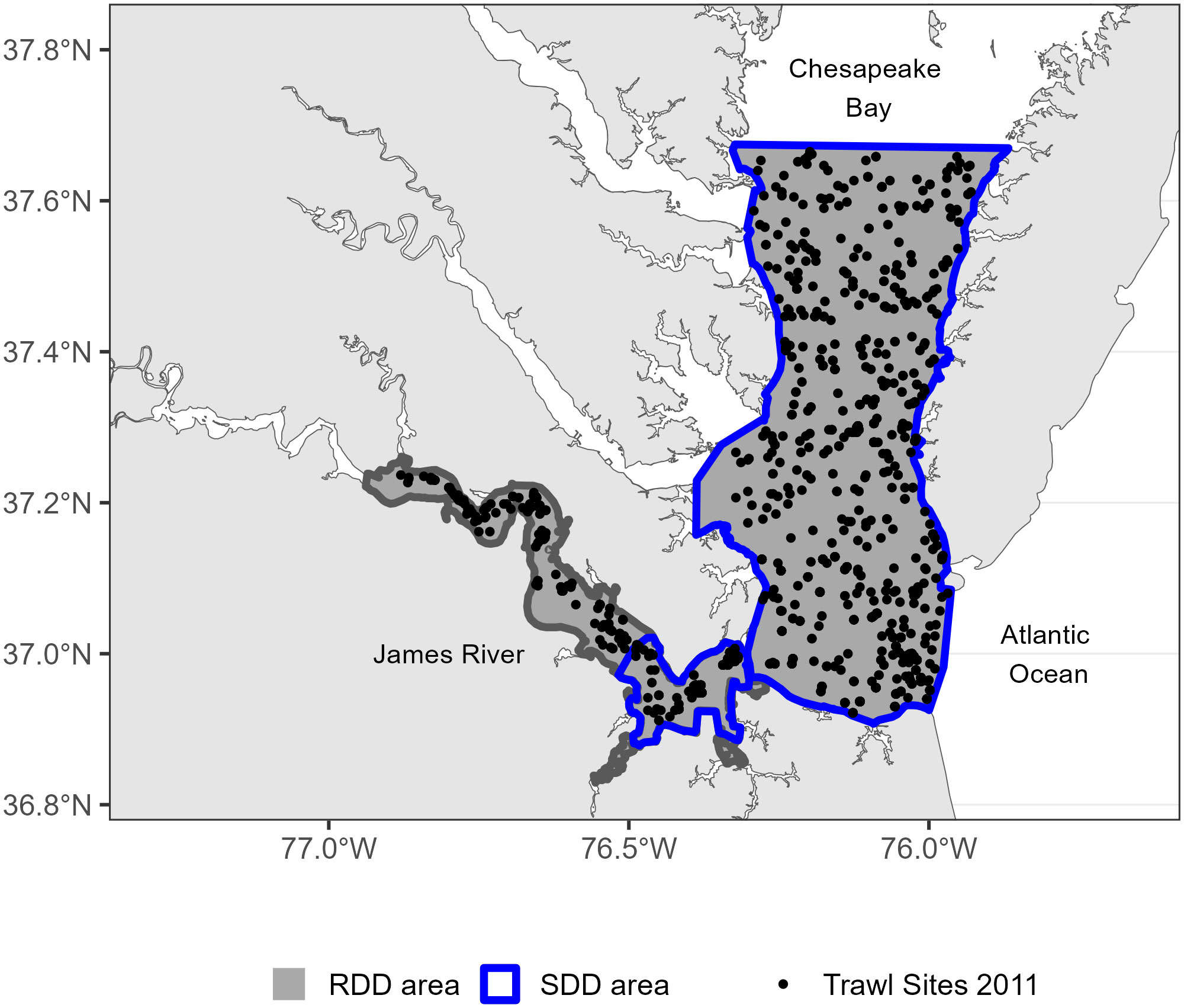
Figure 1 Sampling locations of the Virginia Institute of Marine Science Juvenile Fish Trawl Survey in 2011 for the James River and mainstem of lower Chesapeake Bay in February and April to November. The year 2011 is as an example of the spatial coverage of the trawl survey across months: February, April, May, June, July, August, September, October, and November. Dark gray polygons represent the areas where reproductive degree days (RDD) were calculated. Polygons outlined in blue represent the areas where spawning degree days (SDD) were calculated.
RDD and SDD were calculated for each grid cell in the model; these values were then averaged over the relevant spatial extents in the James River and Chesapeake Bay. Averaging over regions was appropriate for inferences on blue crab spawning because adult females are highly mobile foragers and undergo migrations throughout Chesapeake Bay (Aguilar et al., 2005; Lambert et al., 2006a). To quantify trends in the potential spawning season, annual RDD and SDD estimates for each of the James River and the Virginia portion of the mainstem of the Chesapeake Bay (herein Chesapeake Bay) were modeled as a function of year and region (James or Chesapeake Bay) using weighted linear regression. Weights were defined as the inverse variance of the mean RDD and SDD estimates; a first-order autoregressive correlation structure was used to account for temporal autocorrelation across the time series. Model assumptions were assessed visually using normalized residuals, which satisfied assumptions of normality and homoskedasticity.
2.2 Observed spawning season
Onset, conclusion, and duration of the blue crab spawning season were calculated annually from 1995 to 2019 using counts of ovigerous females from the Virginia Institute of Marine Science Trawl Survey, herein trawl survey (Tuckey and Fabrizio, 2022). The presence of egg-bearing crabs was noted by the trawl survey scientists starting in 1995. From 1995 to 2015, the gear consisted of 9.1-m headline, 4-seam trawl net with a 38.1-mm stretch-mesh body and a 6.4-mm mesh cod liner. Since 2016, the net has had a 5.8-m headline, a 40-mm stretch-mesh body and a 6.4-mm liner. Counts of ovigerous female crabs were adjusted to account for changes in gear (Fabrizio and Tuckey, 2016). The trawl survey is a stratified (by depth and region) random survey, with 5-min tows performed monthly at 22 stations in the James River and 39 to 45 stations in the Virginia portion of the Chesapeake Bay (Figure 1). The trawl survey also samples the York and Rappahannock rivers, however, ovigerous crabs are not reliably encountered in these two rivers, likely due to lower salinities in these regions. Therefore, these regions were excluded from analyses.
Trawl survey sampling occurred monthly, year-round, except for January and March in the Chesapeake Bay. All female crabs captured by the trawl survey were counted, classified as mature or immature based on abdomen shape (Van Engel, 1958), and egg-bearing females were noted. Only catches from February, and April through November were used in the analysis to maintain consistency between sampling months in the James River and the Chesapeake Bay. December was excluded due to concerns about catchability of blue crabs during winter when blue crabs may not be vulnerable to the gear as a result of their burying behavior. Methods for imputation of missing data due to vessel issues or weather conditions are provided in Supplementary Materials (SM) section 1.
Counts of ovigerous female crabs were fit using generalized linear models (GLM) with a negative binomial distribution and log-link, adapted from Edwards and Crone (2021). The GLM was specified as:
where k is the overdispersion parameter for the negative binomial distribution, represents the mean count of egg-bearing female crabs in and , is the intercept and set to 0, is the estimate for the effect of year j as a categorical variable, is the estimate for the interaction effect of where month is a continuous variable, and is the partial regression coefficient for the interaction effect of . Within the model, month acts as the independent variable while year functions as a blocking factor. This model formulation allows the slope and quadratic term to parameterize a Gaussian curve. To obtain a bell-shaped curve, must be negative (see Edwards and Crone, 2021 for full methodological details). This method assumes that the spawning season is unimodal, which is appropriate for blue crabs in Chesapeake Bay (Supplementary Materials (SM) section 2). Model fit was evaluated through visual inspection of residuals as well as the ratio of model deviance to degrees of freedom, which is expected to equal 1 for negative binomial GLMs that fit the data well.
Given that the trawl survey sampling effort has been consistent over the study time frame, using count data in lieu of catch per unit effort was appropriate. To ensure this assumption was reasonable, we compared model estimates for a negative binomial model with and without effort as an offset and found no statistically significant differences in estimates of phenology metrics (Supplementary Materials (SM) section 3).
The parameter estimates from the GLM were used to estimate phenological metrics of the observed spawning season: onset, conclusion and duration of spawning. The months at which 10% and 90% of ovigerous crabs were collected by the survey were considered the spawning onset and spawning conclusion, respectively. Duration was calculated as the time between onset and conclusion. All estimates are presented in months to stay consistent with the trawl survey sampling design. Confidence intervals for the estimates of the phenological metrics were calculated via parametric bootstrapping in which the model variance-covariance matrix was used to estimate a distribution for each model coefficient. The distribution of each model coefficient was sampled 10,000 times for each year and phenological estimates were recalculated from the bootstrap replicates. The variance, 95% confidence interval, and standard error were calculated from the resulting 10,000 phenological estimates. Two statistical models were constructed: one model used counts of ovigerous females from the James River, and the other used counts from Chesapeake Bay. The two areas were evaluated separately to avoid confounding space and time given the sampling design of the trawl survey. Within a given month, the trawl survey does not sample the Chesapeake Bay and James River simultaneously, and the Chesapeake Bay was sampled prior to the James River in most (76%) months sampled in this study.
2.3 Drivers of the observed spawning season
Weighted linear regressions were used to examine the effect of SDD and RDD on spawning onset, conclusion and duration, with the weight equal to the inverse variance of the phenology metric to account for uncertainty in the modeled estimates. The variance of each phenology metric was estimated from the phenological metrics derived from parametric bootstrapping. An additional model of spawning conclusion was constructed using spawning onset as the independent variable. Spring SDD and RDD were used in onset models and were calculated using temperatures from January 1 to April 30. Fall SDD and RDD were used in conclusion models and calculated using temperatures from September 1 to December 31. Annual SDD and RDD were used in duration models and used temperatures from the entire calendar year. Models of the same phenology metric (i.e., onset, conclusion or duration) and region but using SDD or RDD as the independent variable were compared using Akaike’s Information Criterion (AIC, Anderson, 2008).
Linear model performance was evaluated using the deviance explained. Assumptions of normality and homogeneity of variance were assessed visually using normalized residuals. Temporal dependence among phenology metrics was investigated using an autocorrelation function plot. All models used for inference met the assumptions of general linear models.
2.4 Latitudinal differences in potential spawning season
Temperature data from coastal waters in Florida to Maine were retrieved from the National Estuarine Research Reserve System (NERRS). Thirty-two water-quality monitoring buoys spanning 8 states along the native range of the blue crab were selected: Florida, North Carolina, South Carolina, Delaware, New Jersey, Rhode Island, New Hampshire, and Maine (Supplementary Materials (SM) section 4). These states represent areas with NERRS monitoring buoys and either reported distribution shifts of blue crabs (New Hampshire and Maine: Johnson, 2015; Stasse et al., 2023) or areas with considerable research on blue crab spawning (Florida, North Carolina, Chesapeake Bay), as well as outermost states of the east coast of the United States portion of the latitudinal range (Florida and Maine). Monitoring buoys record temperature every 15 minutes. Temperatures from 2015 to 2019 were used in this analysis; temperature observations from two stations in 2015 were omitted due to implausible temperature values (Supplementary Materials (SM) section 4). Daily temperature was calculated by taking the mean of the ~96 temperature readings recorded during each 24-hour period, and the SDD and RDD were calculated for each year and monitoring station based on the average daily temperature. Within a monitoring station, annual degree days for years 2015 to 2019 were averaged to a single estimate. Degree days for the James River and Chesapeake Bay were calculated as described in section 2.1, and the annual degree days from 2015 to 2019 were similarly averaged. The relationship between degree days and latitude was modeled using a simple linear regression. Model estimates of RDD and SDD were compared between North Carolina and the Chesapeake Bay because North Carolina borders Virginia to the south and future Chesapeake Bay conditions are often predicted based on current North Carolina conditions. For example, in 2100, the duration and extent of lethal winter temperatures for blue crabs in Chesapeake Bay are expected to be similar to present day North Carolina temperature regimes (Glandon et al., 2019). Moreover, RDD and spawning activity are positively correlated in North Carolina, allowing for comparisons of reproductive activity across regions (Darnell et al., 2009).
3 Results
3.1 Potential spawning season
The duration of the potential spawning season lengthened significantly from 1985 to 2019 in the James River and Chesapeake Bay (Figure 2, Table 1). Spawning degree days (SDD) increased by 3.6 degree-days y-1 (Table 1), while reproductive degree days (RDD) increased by 5.0 degree-days y-1 (Table 1) in the James River and Chesapeake Bay. Moreover, the duration of the potential spawning season was significantly longer in the James River than in Chesapeake Bay. The James River had 392.9 more SDD (Table 1) and 663.3 more RDD than Chesapeake Bay (Table 1).
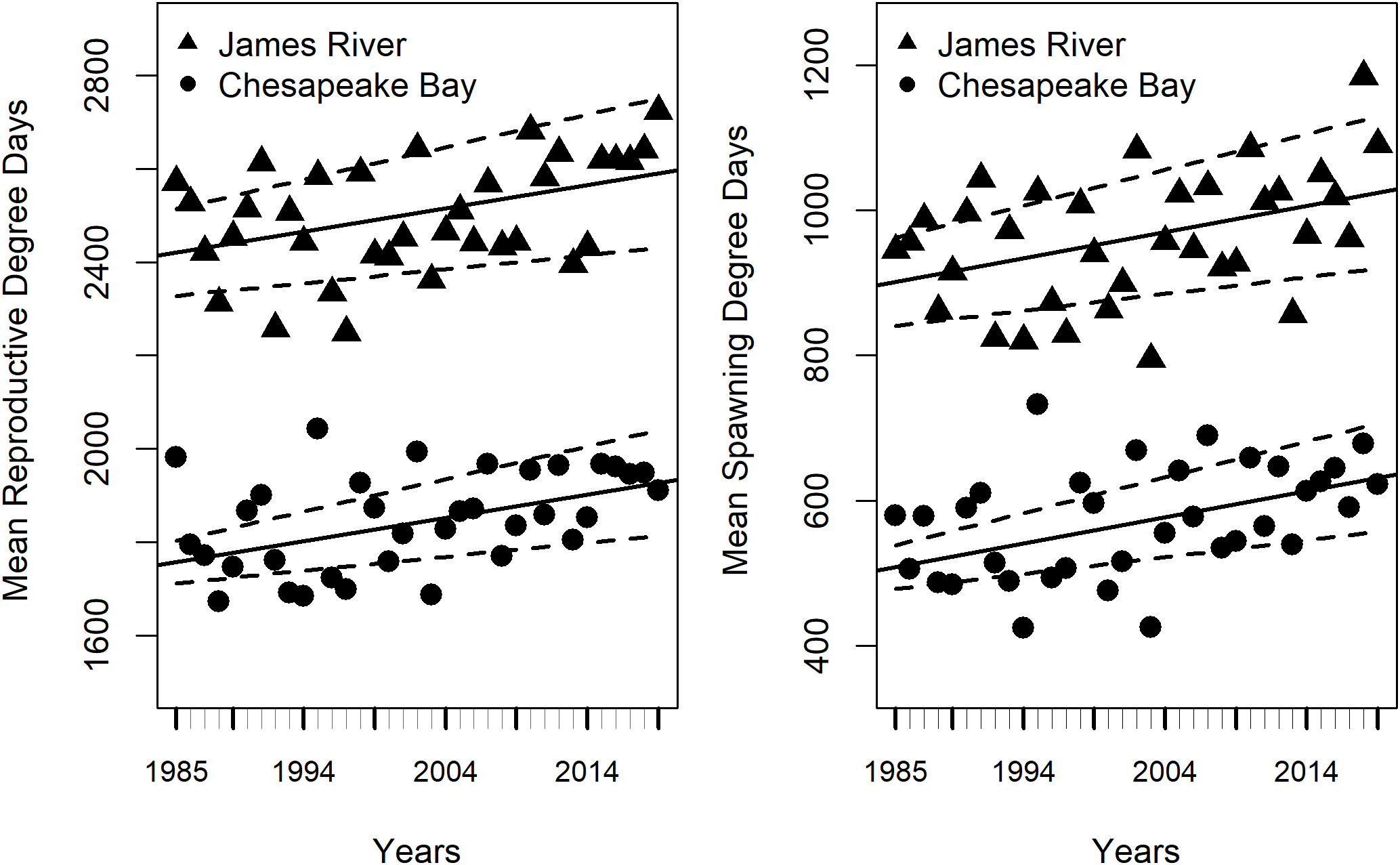
Figure 2 Mean annual reproductive degree days (RDD, left) and spawning degree days (SDD, right) as a function of region and years (1985 to 2019). The James River is represented by triangles and Chesapeake Bay is represented by circles. Black lines represent weighted linear regressions, dashed lines are 95% confidence intervals. Model results are presented in Table 1.
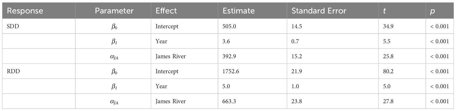
Table 1 Parameter estimates for weighted linear regression models of spawning degree days (SDD) or reproductive degree days (RDD) as a function of year and region from 1985 to 2019 for Chesapeake Bay and the James River (SDD Tmin = 19°C, RDD Tmin = 12°C).
3.2 Observed spawning season
From 1995 to 2019, the trawl survey captured 3,662 ovigerous blue crabs in Chesapeake Bay and 1,705 ovigerous blue crabs in the James River. The negative binomial GLMs visually fit the data well, and our data supported the assumption of a unimodal spawning season (Supplementary Materials (SM) section 2). Over the 25 years, onset of the spawning season occurred earlier in the James River (mean ± SE: 5.13 ± 0.13 months after Jan. 1, which corresponds to early May) than in Chesapeake Bay (mean ± SE: 5.96 ± 0.09 months after Jan. 1, which corresponds to late May to early June, Figure 3). The spawning season also concluded earlier in the James River than in Chesapeake Bay, in mid-July (mean ± SE: 7.58 ± 0.11 months after Jan. 1) and early August (mean ± SE: 8.31 ± 0.11 months after January 1), respectively (Figure 3). Despite differences in onset and conclusion, the duration of the spawning season was about 2.4 months for both the James River and Chesapeake Bay (mean ± SE: 2.44 ± 0.12 and 2.35 ± 0.08), respectively (Figure 3), which reflected a difference of only 3 days.
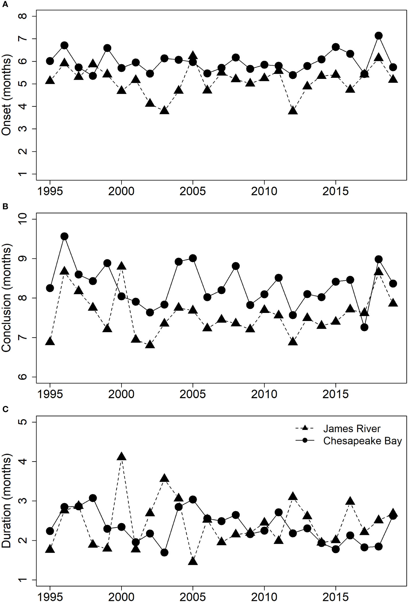
Figure 3 Estimates of the observed spawning season (A) onset, (B) conclusion, and (C) duration in months since January 1 from 1995 to 2019. The James River is represented by triangles and the Chesapeake Bay is represented by circles.
3.3 Drivers of the observed spawning season
Model comparisons of spawning phenology for the James River and Chesapeake Bay were similar across areas based on AIC. Month of spawning onset was best predicted by spring RDD and spawning conclusion was best predicted by spawning onset (Table 2). In both the James River and Chesapeake Bay, month of spawning onset was earlier in years with greater spring RDD (Table 3, Figure 4), and month of spawning conclusion occurred earlier in the year when the month of spawning onset was earlier (Table 4, Figure 5). In the James River, spawning conclusion was also later in the year when fall SDD and RDD were high, neither of which was significantly related to spawning season conclusion in Chesapeake Bay (Supplementary Materials (SM) section 5). In Chesapeake Bay, the best predictor of spawning duration was annual RDD (Table 2), although years with increased RDD had shorter spawning durations (Table 5, Figure 6). In the James River, annual RDD and SDD were poor predictors of spawning duration (Supplementary Materials (SM) section 5).
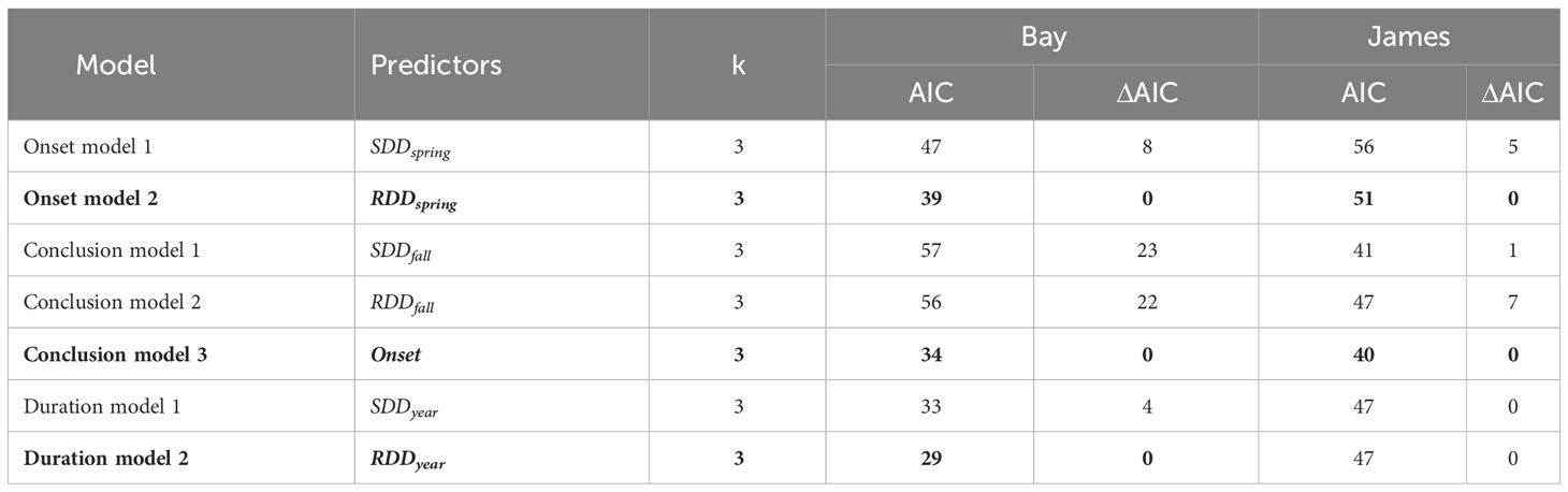
Table 2 Hypothesized onset models and Akaike’s Information Criteria (AIC), for the Chesapeake Bay mainstem (Bay) and James River (ΔAIC represents the difference in AIC values between a given model and the model with the lowest AIC within model groupings). k is the number of parameters in the model including the intercept and variance. SDD, spawning degree days and RDD, reproductive degree days. Onsets are regressed as a function of spring degree days (Jan. 1 – April 30), conclusions are regressed as a function of fall degree days (Sept. 1 – Dec. 31), and durations are regressed as a function of annual degree days. The top performing model, based on AIC, is in bold font.
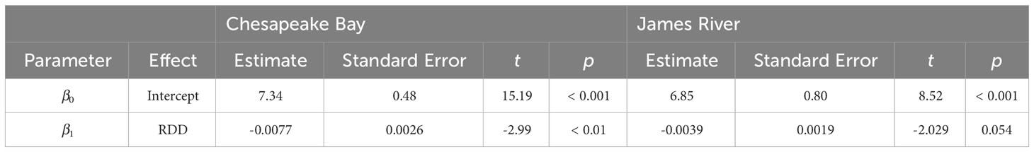
Table 3 Parameter estimates from weighted linear regression models of spawning season onset in Chesapeake Bay (r2 = 0.28) and the James River (r2 = 0.15) as a function of spring reproductive degree days (RDD, calculated from Jan. 1 – April 30).
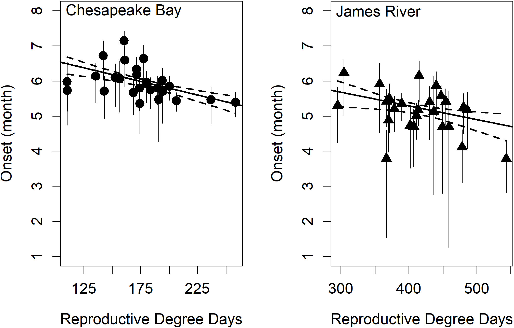
Figure 4 The effect of reproductive degree days on spawning onset in Chesapeake Bay (left) and James River (right). Chesapeake Bay is represented by circles and the James River is represented by triangles. Dashed lines are the 95% confidence interval for the linear model (black regression line, r2Bay = 0.28 and r2James = 0.15) and vertical error bars represent 95% confidence intervals in the estimate of the phenology metric.
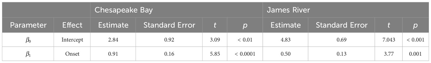
Table 4 Parameter estimates from weighted linear regression models of spawning season conclusion in Chesapeake Bay (r2 = 0.60) and the James River (r2 = 0.38) as a function of spawning season onset.
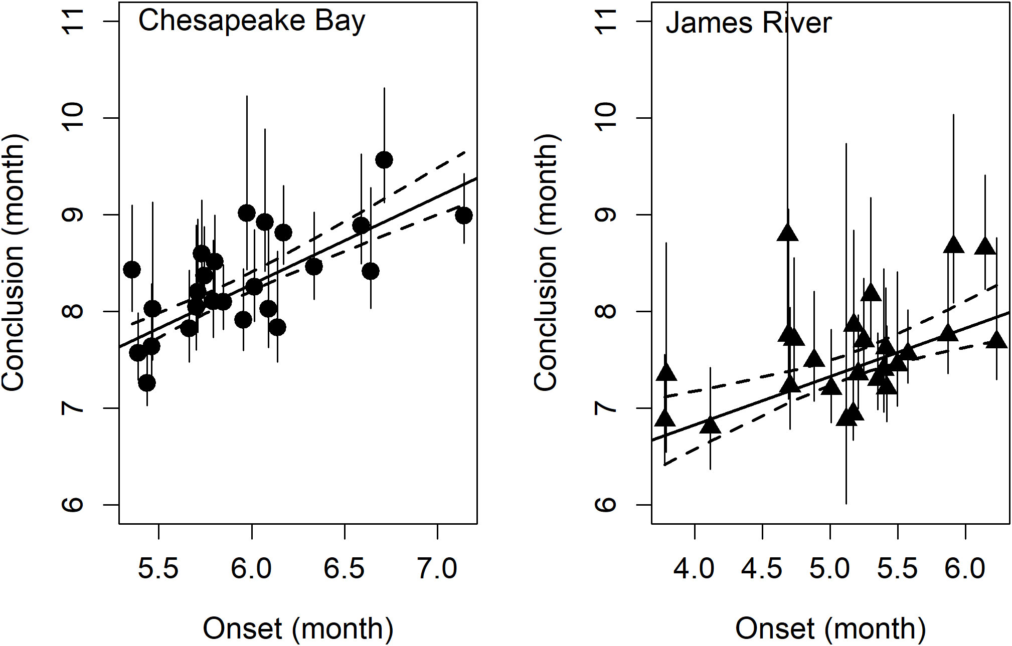
Figure 5 The effect of spawning onset on spawning conclusion in Chesapeake Bay (left) and James River (right). Dashed lines are the 95% confidence interval for the linear model (black regression line, r2Bay = 0.60 and r2James = 0.38) and vertical error bars represent 95% confidence intervals in the estimate of the phenology metric.
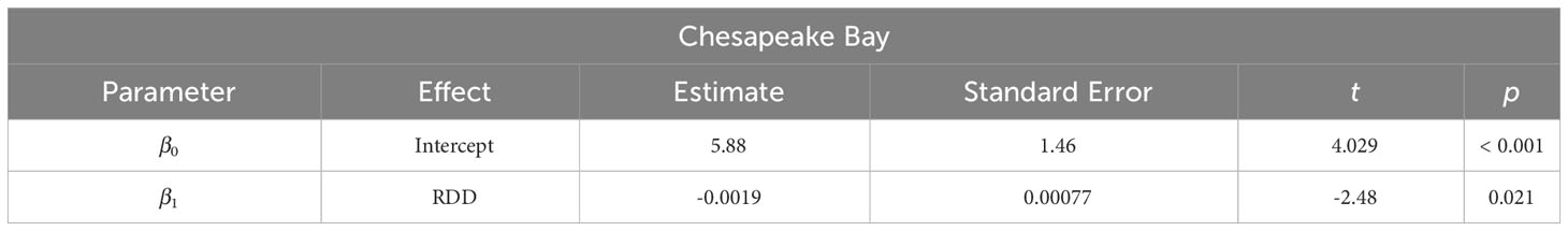
Table 5 Parameter estimates from weighted linear regression models of spawning season duration in Chesapeake Bay (r2 = 0.21) as a function of annual reproductive degree day (RDD, calculated from Jan. 1 – Dec. 31).
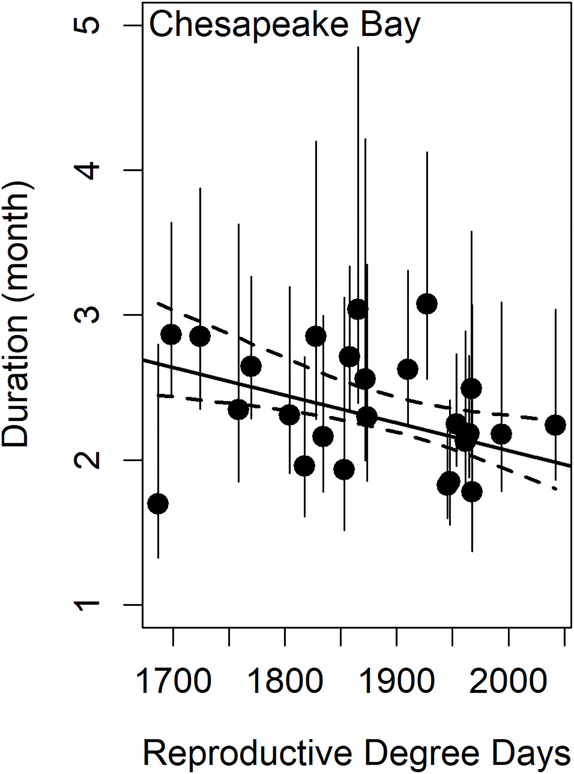
Figure 6 The effect of reproductive degree days on spawning duration in Chesapeake Bay. Dashed lines are the 95% confidence interval for the linear model (black regression line, r2 = 0.21) and vertical error bars represent 95% confidence intervals in the estimate of the phenology metric.
3.4 Latitudinal differences in potential spawning season
As hypothesized, RDD and SDD were strongly linearly related with latitude (linear model: r2 = 0.95 and r2 = 0.93, respectively; Figure 7; Supplementary Materials Figure 6). Based on the slope parameters, SDD decreased by 125.6 degree days and RDD decreased by 223.7 degree days per unit increase in latitude (Figure 7, Supplementary Materials (SM) section 6). North Carolina had 383 more SDD and 683 more RDD than Chesapeake Bay. Given our estimates of the rates of change for RDD and SDD in Chesapeake Bay (Table 1), the Bay region will reach the RDD and SDD for North Carolina in 137 y and 106 y, respectively, assuming rates of temperature change remain constant.
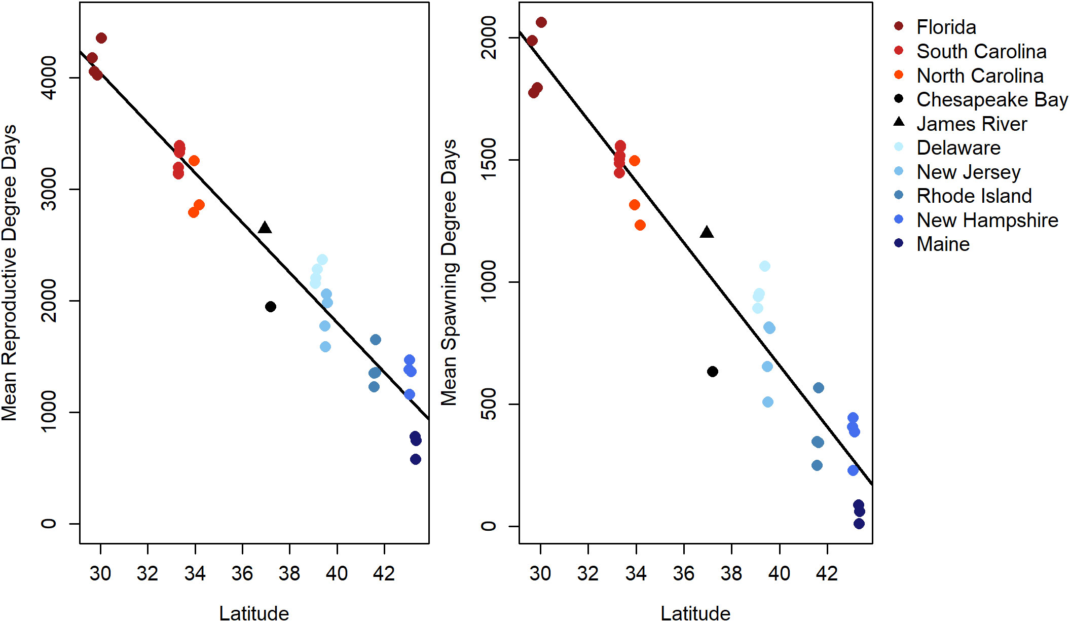
Figure 7 Mean reproductive degree days (RDD, left) and mean spawning degree days (SDD, right) estimated from temperature data collected by monitoring buoys in coastal waters along the East Coast of the U.S. Means represent annual degree days averaged from 2015 to 2019. All temperature data were retrieved from the National Estuarine Research Reserve System (Supplementary Materials (SM) section 4), except Chesapeake Bay and James River data which were calculated as described in section 2.1. Black lines are simple linear regressions of degree days as a function of latitude (RDD = 10743.5 – 223.7 × Lat, r2RDD = 0.95; and SDD = 5674.3 – 125.6 × Lat, r2SDD = 0.93).
4 Discussion
From 1985 to 2019, the duration of the potential spawning season, measured with degree days, increased, although the duration of the observed spawning season had no temporal trend. Rather the observed month of spawning onset was driven by RDD in spring, whereby a greater accumulation of RDD in the beginning of the year led to an earlier spawning onset. We found that the conclusion of spawning was positively related to the onset of spawning, such that the duration of the observed spawning season did not change for the blue crab in Chesapeake Bay or the James River. Increasing trends in RDD and SDD reflect the warming of Chesapeake Bay and an expansion of the potential spawning season. From 1985 to 2019, degree days increased by about 25% SDD and 10% RDD, but these temporal trends were not reflected in the fishery-independent observations of blue crab spawning phenology. In this study, we demonstrated that the spawning season currently lasts approximately 2.4 months, but spawning begins and concludes earlier in years with warmer springs. Notably, in these warmer springs, spawning onset can occur before the blue crab spawning sanctuary is in effect. Intense female harvest in spring may reduce reproductive output of female crabs in the Chesapeake Bay by removing females before they have the opportunity to spawn. As warming continues, female spawners may become more vulnerable to fishing during warm springs, prior to the onset of the spawning season and the closure of the spawning sanctuary.
4.1 Implications for blue crab reproduction
Temperature regimes differed substantially between North Carolina and Chesapeake Bay, as reflected in a longer spawning season and greater brood production in North Carolina (Dickinson et al., 2006; Darnell et al., 2009). Considerable warming is required before Chesapeake Bay females can produce broods at the annual rate currently observed in North Carolina. In North Carolina, females produce their first egg mass within 747 RDD of mating and have an average brood production interval of 263 RDD per brood, giving them the potential to produce eight broods per spawning season (Dickinson et al., 2006; Darnell et al., 2009). The average annual RDD in Chesapeake Bay from 2015 to 2019 was about 1,800 RDD (Figure 7, Supplementary Table 5), which would allow Chesapeake Bay females to produce up to four broods per spawning season, assuming their brood production per RDD is equivalent to females in North Carolina (Darnell et al., 2009). This is a slightly higher estimate than the two to three broods currently observed. Since 1958, females in the Chesapeake Bay have been assumed to spawn one to three times per year (Van Engel, 1958). In North Carolina the average RDD from 2015 to 2019 was about 3,000, suggesting that females could produce up to eight broods, which is greater than the observed maximum of seven broods per female over one to two spawning seasons (Dickinson et al., 2006; Darnell et al., 2009). Therefore, estimates of brood production using degree days appear to overestimate annual brood production. Moreover, reproductive timing alone may not dictate the number of sponges, which may be affected by additional factors such as sperm limitation and lifespan (Hines et al., 2003; Darnell et al., 2009). Additional field studies are needed to quantify the number of broods produced by female blue crabs in Chesapeake Bay and how increases in temperature may affect brood production.
4.2 Spawning season trends
The lack of temporal trends in the observed phenological metrics (i.e., onset, conclusion and duration of spawning) was contrary to what we hypothesized for blue crabs in Chesapeake Bay. Our results, however, indicate that spawning season onset was significantly advanced by warmer spring temperatures, and since temperatures are rising, future warming will likely produce consistently early spawning onset and possibly a longer spawning duration. Phenological shifts have occurred in other species in Chesapeake Bay, such as cobia Rachycentron canadum (Crear et al., 2020), and in other decapod species, such as American lobster Homarus americanus in the Gulf of St. Lawrence (Haarr et al., 2020) and northern shrimp Pandalus borealis in the Gulf of Maine (Richards, 2012). Moreover, we expect blue crabs, being a short-lived, r-selected species, to respond rapidly to shifts in temperature (Perry et al., 2005). Our results indicate that a unidirectional phenological shift in blue crab reproduction in mid-latitude systems may not be apparent over a 25-year time period with gradual increases in ambient temperature. Our observation is consistent with Poloczanska et al. (2016) who reported phenological shifts in mid-latitudes are slower than phenological shifts at high and low latitudes. Responses to climate change have been documented for the blue crab at higher latitudes, such as range expansions into regions that historically were too cold to maintain permanent or reproducing populations (Johnson, 2015; Stasse et al., 2023).
The lack of an observed unidirectional temporal trend in the blue crab spawning season in Chesapeake Bay may simply reflect the abridged time series that we analyzed (1995 to 2019). Additional years of trawl survey data may be needed to observe a temporal pattern, because the length of the time series is a significant predictor in detecting phenological shifts (Bush et al., 2018). Moreover, the relationship between RDD and year is subtle (5 RDD per year), and the trawl survey sampling design may be too temporally coarse to detect slow changes in the onset or conclusion of the spawning season in Chesapeake Bay. In addition, the percent increase in temperature rise was greater for SDD than RDD, which aligns with a higher rate of warming in summer than the remainder of the year (Hinson et al., 2021). RDD was a clearer predictor of phenology metrics than SDD; therefore, spring and fall warming may be more important in altering blue crab spawning phenology than higher summer temperatures. Temperature is a major driver of female blue crab spawning frequency (Bembe et al., 2017), such that expansion of spawning season duration may become more pronounced as warming continues.
The onset and conclusion of the spawning season differed notably between the James River and Chesapeake Bay. The spawning season began and ended three to four weeks earlier in the James River than in Chesapeake Bay, likely due to earlier warming and cooling in the James River. The James River is shallower than Chesapeake Bay and is therefore more strongly influenced by air temperature (Hinson et al., 2021). Moreover, Chesapeake Bay receives a greater influx of cooler ocean water than the James River throughout the year. The earlier spawning season conclusion in the James River than in Chesapeake Bay may also have been related to air temperature, because the James River cools more quickly than Chesapeake Bay in fall. This is supported by the positive, significant relationship between SDD or RDD and spawning conclusion in the James River. Additionally, there may be a delayed conclusion of the spawning season in the James River because the ovigerous crabs from the James River are assumed to migrate to the mouth of the Chesapeake Bay to hatch their eggs after spawning in the lower James River. However, mature females on the spawning grounds return to the lower James River to feed in the shallow high salinity areas between broods (Lambert et al., 2006a), and therefore a unidirectional movement of mature or egg-bearing females out of the Chesapeake Bay tributaries may not characterize the James River.
The earlier onset and conclusion of the spawning season in the James River may also have been influenced by the sampling design of the trawl survey. On average, Chesapeake Bay is sampled 5.7 d earlier than the James River. In spring, sampling in the Chesapeake Bay may occur prior to the onset of spawning, whereas sampling the James River later in the same month increases the odds of encountering an ovigerous crab in any given month. A similar phenomenon may occur in the fall: the later sampling in the James River could decrease the probability of encountering an ovigerous female, leading to an earlier estimate of spawning season conclusion. Conversely, earlier sampling in Chesapeake Bay could cause estimates in the Bay to be earlier if spawning begins concurrently in Chesapeake Bay and the James River. Unfortunately, we were unable to test these potential biases with the available data. We believe that the magnitude of difference between spawning metrics (3-4 weeks) in the James River and Chesapeake Bay compared to the average difference in sampling time (5.7 d) reduces the likelihood that the sampling design is a major driver in the regional differences between phenological estimates.
The James River had greater uncertainty in phenology metrics than Chesapeake Bay, likely due to the lower number of ovigerous crabs encountered in the James River. Specifically, the variances of the onset estimates were greater for the James River (mean var = 1.1) and lower for the Chesapeake Bay (mean var = 0.1); uncertainty estimates for other phenology metrics exhibited the same pattern. The lower catches of ovigerous crabs in the James River are likely related to the smaller area of the James River, the declining salinities in upriver sections, and the fewer trawl tows performed in the James River. Catches of egg-bearing crabs in Chesapeake Bay between 1995 and 2019 were more than double those in the James River. Years with the lowest catches in the James River, such as 1995 (n = 4), 2000 (n = 19) and 2005 (n = 21), had high uncertainty in the estimates of onset and conclusion. Years with low total counts were also more influenced by observations of one or two egg-bearing crabs in early and late spawning months, such as November. This may have contributed to differences in the effect sizes between the James River and Chesapeake Bay.
4.3 Fishery implications
Female crabs in the James River are vulnerable to fishing during the entire commercial crabbing season, while females in the spawning sanctuary in the Chesapeake Bay are protected from harvest from mid-May to mid-September. Females in the James River will molt to maturity, mate, and migrate to high salinity areas from spring through fall. After their migration to the lower Chesapeake Bay and between broods, adult females forage in shallow, high salinity areas, including the lower James River (Lambert et al., 2006a), making them vulnerable to fishing. Within Chesapeake Bay, the onset of the observed spawning season now begins prior to the sanctuary closure dates (May 16 for the majority of the sanctuary) in at least 20% of the years examined. When we used a lower quantile to estimate spawning onset (i.e., 2.5% quantile instead of the 10% quantile described in section 2.2), the spawning season was estimated to begin before the sanctuary was closed to fishing in 72% of years. This implies that a sizable portion of the female spawners in any given year will be vulnerable to harvest prior to the close of fishing in the sanctuary. Most mature females in spring have not yet spawned and will begin their first spawning season (Schneider et al., 2023) by producing their largest and most viable egg clutch (Darnell et al., 2009; Graham et al., 2012). High fishing mortality rates on these females (primiparous, first-year spawners) during spring may thus decrease population-level reproductive output substantially (Schneider et al., 2023).
Our results justify further protection of female crabs in April and May to ensure the highest level of egg production prior to their harvest. As warming continues and spawners become more active earlier in spring, phenological shifts in reproduction will become more pronounced. Shifts in species phenology or distribution in response to climate change can decrease the efficacy of marine sanctuaries (Van Keeken et al., 2007), such as the blue crab spawning sanctuary (Lipcius et al., 2003; Lambert et al., 2006b) and increase the risk of exploitation, which may be the case here. The lack of expansion of the duration of the observed spawning season suggests that warming has not progressed enough in Chesapeake Bay to allow for additional broods to be produced by females later in the year. Globally, our study informs how warming is impacting the timing of reproduction of an economically important decapod species. Locally, our study allows managers to consider the effects of spring warming on the efficacy of the spawning sanctuary. A greater fraction of the spawning stock could be protected by earlier closure to fishing in the spawning sanctuary, or by reduction of fishing effort in the spring before the sanctuary closes.
Data availability statement
Publicly available datasets were analyzed in this study. This data can be found as follows. The temperature data for Chesapeake Bay from Hinson et al. (2021) can be accessed through William & Mary ScholarWorks here: [https://scholarworks.wm.edu/data/430/]. The NERRS data are available from the NERRS website: [https://cdmo.baruch.sc.edu/get/landing.cfm]. The counts of ovigerous crabs, adjusted for vessel and gear changes, are available at William & Mary ScholarWorks here: [https://scholarworks.wm.edu/data/675/].
Ethics statement
The manuscript presents research on animals that do not require ethical approval for their study.
Author contributions
AS: Conceptualization, Formal Analysis, Investigation, Methodology, Visualization, Writing – original draft, Data curation, Funding acquisition, Project administration. MF: Conceptualization, Data curation, Funding acquisition, Investigation, Supervision, Writing – review & editing, Formal Analysis, Methodology, Resources. RL: Conceptualization, Investigation, Supervision, Writing – review & editing, Formal Analysis, Funding acquisition, Methodology.
Funding
The author(s) declare financial support was received for the research, authorship, and/or publication of this article. This research was made possible by the Willard A. Van Engel Fellowship, as well as a Virginia Sea Grant Graduate Fellowship under Grant #V721500, Virginia Sea Grant College Program Project No. 222030, from the National Oceanic and Atmospheric Administration’s (NOAA) National Sea Grant College Program, U.S. Department of Commerce. The Trawl Survey is supported by the Virginia Marine Resources Commission, the Commonwealth of Virginia, the US Fish & Wildlife Service, and VIMS.
Acknowledgments
This project was possible thanks to the contribution of many individuals who participated in the VIMS Trawl Survey (particularly J. Buchanan, A. Comer, S. Dowiarz, W. Lowery, K. Nickerson, D. Royster, and T. Tuckey). Special thanks to K. Hinson for help accessing and working with the temperature data from the ROMS model. Access to coast-wide temperature data was possible thanks to the National Estuarine Research Reserves monitoring programs. We thank A.C. Hyman and G. Ralph for their constructive feedback on this paper as well as J.D. Shields, M. Ogburn and R.D. Seitz for feedback as members of A.K. Schneider’s graduate committee.
Conflict of interest
The authors declare that the research was conducted in the absence of any commercial or financial relationships that could be construed as a potential conflict of interest.
The author(s) declared that they were an editorial board member of Frontiers, at the time of submission. This had no impact on the peer review process and the final decision.
Publisher’s note
All claims expressed in this article are solely those of the authors and do not necessarily represent those of their affiliated organizations, or those of the publisher, the editors and the reviewers. Any product that may be evaluated in this article, or claim that may be made by its manufacturer, is not guaranteed or endorsed by the publisher.
Author disclaimer
The statements, findings, conclusions, and recommendations are those of the authors and do not necessarily reflect the views of Virginia Sea Grant, NOAA, or the U.S. Department of Commerce.
Supplementary material
The Supplementary Material for this article can be found online at: https://www.frontiersin.org/articles/10.3389/fevo.2023.1304021/full#supplementary-material
References
Aguilar R., Hines A. H., Wolcott T. G., Wolcott D. L., Kramer M. A., Lipcius R. N. (2005). The timing and route of movement and migration of post-copulatory female blue crabs, Callinectes sapidus Rathbun, from the upper Chesapeake Bay. J. Exp. Mar. Bio. Ecol. 319, 117–128. doi: 10.1016/j.jembe.2004.08.030
Alaska Department of Fish and Game (2021) Statewide king and tanner crab commercial fishing regulations. Available at: https://salmonbook.alaska.gov/index.cfm?adfg=fishregulations.commercial.
Anderson D. R. (2008). Model based inference in the life sciences a primer of evidence. (New York: Springer).
Anderson J. J., Gurarie E., Bracis C., Burke B. J., Laidre K. L. (2013). Modeling climate change impacts on phenology and population dynamics of migratory marine species. Ecol. Model. 264, 83–97. doi: 10.1016/j.ecolmodel.2013.03.009
Atkinson D. (1994). Temperature and organism size- a law for ectotherms? Adv. Ecol. Res. 25, 1–58. doi: 10.1016/S0065-2504(08)60212-3
Atlantic States Marine Fisheries Commission (2020) Interstate Fishery Management Plan for American Lobster (Homarus americanus). Available at: https://www.asmfc.org/species/american-lobster#management.
Bembe S., Liang D., Chung J. S. (2017). Optimal temperature and photoperiod for the spawning of blue crab, Callinectes sapidus, in captivity. Aquac. Res. 48, 5498–5505. doi: 10.1111/are.13366
Brown J. H., Gilooly J. F., Allen A. P., Savage V. M., West G. B. (2004). Toward a metabolic theory of ecology. Ecology 85, 1771–1789. doi: 10.1007/978-3-031-19410-8_9
Brown C. J., O’Connor M. I., Poloczanska E. S., Schoeman D. S., Buckley L. B., Burrows M. T., et al. (2016). Ecological and methodological drivers of species’ distribution and phenology responses to climate change. Glob. Change Biol. 22, 1548–1560. doi: 10.1111/gcb.13184
Brylawski B. J., Miller T. J. (2006). Temperature-dependent growth of the blue crab (Callinectes sapidus): a molt process approach. Can. J. Fish. Aquat. Sci. 63, 1298–1308. doi: 10.1139/f06-011
Burrows M. T., Schoeman D. S., Buckley L. B., Moore P., Poloczanska E. S., Brander K. M., et al. (2011). The pace of shifting climate in marine and terrestrial ecosystems. Science 334, 652–656. doi: 10.1126/science.1210288
Bush E. R., Bunnefeld N., Dimoto E., Dikangadissi J. T., Jeffery K., Tutin C., et al. (2018). Towards effective monitoring of tropical phenology: maximizing returns and reducing uncertainty in long-term studies. Biotropica 50, 455–464. doi: 10.1111/btp.12543
Cayton H. L., Haddad N. M., Gross K., Diamond S. E., Ries L. (2015). Do growing degree days predict phenology across butterfly species? Ecology 96, 1473–1479. doi: 10.1890/15-0131.1
Chesapeake Bay Program. (2020). Chesapeake assessment and scenario tool (CAST) version 2019 (Chesapeake Bay Program Office). Available at: https://cast.chesapeakebay.net/.
Crear D. P., Watkins B. E., Friedrichs M. A. M., St-Laurent P., Weng K. C. (2020). Estimating shifts in phenology and habitat use of cobia in Chesapeake Bay under climate change. Front. Mar. Sci. 7. doi: 10.3389/fmars.2020.579135
Cushing D. H. (1990). Plankton production and year-class strength in fish populations: An update of the match/mismatch hypothesis. Adv. Mar. Biol. 26, 249–293. doi: 10.1016/S0065-2881(08)60202-3
Damien M., Tougeron K. (2019). Prey–predator phenological mismatch under climate change. Curr. Opin. Insect Sci. 35, 60–68. doi: 10.1016/j.cois.2019.07.002
Darnell M. Z., Rittschof D., Darnell K. M., McDowell R. E. (2009). Lifetime reproductive potential of female blue crabs Callinectes sapidus in North Carolina, USA. Mar. Ecol. Prog. Ser. 394, 153–163. doi: 10.3354/meps08295
Dickey M. H., Gauthier G., Cadieux M. C. (2008). Climatic effects on the breeding phenology and reproductive success of an arctic-nesting goose species. Glob. Change Biol. 14, 1973–1985. doi: 10.1111/j.1365-2486.2008.01622.x
Dickinson G. H., Rittschof D., Latanich C. (2006). Spawning biology of the blue crab, Callinectes sapidus, in North Carolina. Bull. Mar. Sci. 79, 273–285.
Doney S. C., Ruckelshaus M., Emmett D. J., Barry J. P., Chan F., English C. A., et al. (2012). Climate change impacts on marine ecosystems. Ann. Rev. Mar. Sci. 4, 11–37. doi: 10.1146/annurev-marine-041911-111611
Edwards C., Crone E. E. (2021). Estimating abundance and phenology from transect count data with GLMs. Oikos 130, 1335–1345. doi: 10.1111/oik.08368
Edwards M., Richardson A. J. (2004). Impact of climate change on marine phenology and trophic mismatch. Nature 430, 881–884. doi: 10.1038/nature02808
Elith J., Leathwick J. R. (2009). Species distribution models: Ecological explanation and prediction across space and time. Annu. Rev. Ecol. Evol. Syst. 40, 677–697. doi: 10.1146/annurev.ecolsys.110308.120159
Fabrizio M. C., Tuckey T. D. (2016). Calibration of VIMS research vessel catch data to ensure continuity of recruitment indices for the Chesapeake Bay (Gloucester Point, VA: Virginia Institute of Marine Science, William & Mary). doi: 10.21220/V5QC7B
Fogarty M. J., Lipcius R. N. (2007). “Population dynamics and fisheries,” in Blue crab: Callinectes sapidus. Eds. Kennedy V. S., Cronin L. E. (College Park, MD: Maryland Sea Grant College), 711–755. S.
Franke J. A., Müller C., Minoli S., Elliott J., Folberth C., Gardner C., et al. (2022). Agricultural breadbaskets shift poleward given adaptive farmer behavior under climate change. Glob. Change Biol. 28, 167–181. doi: 10.1111/gcb.15868
Glandon H. L., Kilbourne K. H., Miller T. J. (2019). Winter is (not) coming: warming temperatures will affect the overwinter behavior and survival of blue crab. PloS One 14, e0219555. doi: 10.1371/journal.pone.0219555
Graham D. J., Perry H., Biesiot P., Fulford R. (2012). Fecundity and egg diameter of primiparous and multiparous blue crab Callinectes sapidus (Brachyura: Portunidae) in Mississippi waters. J. Crustac. Biol. 32, 49–56. doi: 10.1163/193724011X615325
Grigorieva E. A., Matzarakis A., De Freitas C. R. (2010). Analysis of growing degree-days as a climate impact indicator in a region with extreme annual air temperature amplitude. Clim. Res. 42, 143–154. doi: 10.3354/cr00888
Haarr M. L., Comeau M., Chassé J., Rochette R. (2020). Early spring egg hatching by the American lobster (Homarus americanus) linked to rising water temperature in autumn. ICES J. Mar. Sci. 77, 1685–1697. doi: 10.1093/icesjms/fsaa027
Hart H. R., Crowley C. E., Walters E. A. (2021). Blue crab spawning and recruitment in two Gulf Coast and two Atlantic estuaries in Florida. Mar. Coast. Fish. 13, 113–130. doi: 10.1002/mcf2.10136
Hartnoll R. G. (1985). “Growth, sexual maturity and reproductive output,” in Factors in Adult Growth. Ed. Wenner A. M. (London, UK: Routledge), 101–128.
Hines A. H., Jivoff P. R., Bushmann P. J., Van Montfrans J., Reed S. A., Wolcott D. L., et al. (2003). Evidence for sperm limitation in the blue crab, Callinectes sapidus. Bull. Mar. Sci. (Alaska Sea Grant, University of Alaska Fairbanks) 72, 287–310. doi: 10.4027/bmecpcc.2010.22
Hines A. H., Johnson E. G., Darnell M. Z., Rittschof D., Miller T. J., Bauer L. J., et al. (2011). “Predicting effects of climate change on blue crabs in Chesapeake Bay,” in Biology and management of exploited crab populations under climate change (Anchorage, AK: Alaska Sea Grant, University of Alaska Fairbanks), 109–127. doi: 10.4027/bmecpcc.2010.22
Hinson K. E., Friedrichs M. A. M., St-Laurent P., Da F., Najjar R. G. (2021). Extent and causes of Chesapeake Bay warming. J. Am. Water Resour. Assoc. 58, 1–21. doi: 10.1111/1752-1688.12916
Hood R. R., Shenk G. W., Dixon R. L., Smith S. M. C., Ball W. P., Bash J. O., et al. (2021). The Chesapeake Bay Program Modeling System: Overview and recommendations for future development. Ecol. Model. 456, 109635. doi: 10.1016/j.ecolmodel.2021.109635
Huntley B., Collingham Y. C., Green R. E., Hilton G. M., Rahbek C., Willis S. G. (2006). Potential impacts of climatic change upon geographical distributions of birds. Ibis (Lond. 1859). 148, 8–28. doi: 10.1111/j.1474-919X.2006.00523.x
Johnson D. S. (2015). The savory swimmer swims north: A northern range extension of the blue crab Callinectes sapidus? J. Crustac. Biol. 35, 105–110. doi: 10.1163/1937240X-00002293
Johnston K. M., Freund K. A., Schmitz O. J. (2012). Projected range shifting by montane mammals under climate change: Implications for Cascadia’s National Parks. Ecosphere 3, 1–51. doi: 10.1890/es12-00077.1
Lambert D. M., Hoenig J. M., Lipcius R. N. (2006a). Tag return estimation of annual and semiannual survival rates of adult female blue crabs. Trans. Am. Fish. Soc 135, 1592–1603. doi: 10.1577/t05-318.1
Lambert D. M., Lipcius R. N., Hoenig J. M. (2006b). Assessing effectiveness of the blue crab spawning stock sanctuary in Chesapeake Bay using tag-return methodology. Mar. Ecol. Prog. Ser. 321, 215–225. doi: 10.3354/meps321215
Last P. R., White W. T., Gledhill D. C., Hobday A. J., Brown R., Edgar G. J., et al. (2011). Long-term shifts in abundance and distribution of a temperate fish fauna: A response to climate change and fishing practices. Glob. Ecol. Biogeogr. 20, 58–72. doi: 10.1111/j.1466-8238.2010.00575.x
Linton D. M., Macdonald D. W. (2018). Spring weather conditions influence breeding phenology and reproductive success in sympatric bat populations. J. Anim. Ecol. 87, 1080–1090. doi: 10.1111/1365-2656.12832
Lipcius R. N., Stockhausen W. T., Seitz R. D., Geer P. J. (2003). Spatial dynamics and value of a marine protected area and corridor for the blue crab spawning stock in Chesapeake Bay. Bull. Mar. Sci. 72, 453–470.
McGeady R., Lordan C., Power A. M. (2020). Shift in the larval phenology of a marine ectotherm due to ocean warming with consequences for larval transport. Limnol. Oceanogr 66, 1–15. doi: 10.1002/lno.11622
Miller T. J., Wilberg M. J., Colton A. R., Davis G. R., Sharov A., Lipcius R. N., et al. (2011). Stock assessment of the blue crab in Chesapeake Bay (Solomons, MD: University of Maryland Technical Report Series TS-614-11), 203 pp.
Mills K. E., Pershing A. J., Brown C. J., Chen Y., Chiang F. S., Holland D. S., et al. (2013). Fisheries management in a changing climate: Lessons from the 2012 ocean heat wave in the Northwest Atlantic. Oceanography 26, 191–195. doi: 10.5670/oceanog.2013.27
NOAA National Estuarine Research Reserve System (NERRS). System-wide Monitoring Program. Data accessed from the NOAA NERRS Centralized Data Management Office. Available at: http://www.nerrsdata.org/ (Accessed April 13, 2023).
Nye J. A., Link J. S., Hare J. A., Overholtz W. J. (2009). Changing spatial distribution of fish stocks in relation to climate and population size on the Northeast United States continental shelf. Mar. Ecol. Prog. Ser. 393, 111–129. doi: 10.3354/meps08220
Oregon Department of Fish and Wildlife (2022). Oregon dungeness crab fishery management plan (Newport, OR: Oregon Dept. of Fish and Wildlife). Available at: http://www.dfw.state.or.us/MRP/.
Parmesan C. (2006). Ecological and evolutionary responses to recent climate change. Annu. Rev. Ecol. Evol. Syst. 37, 637–669. doi: 10.2307/annurev.ecolsys.37.091305.30000024
Perry A., Low P., Ellis J., Reynolds J. (2005). Climate change and distribution shifts in marine fishes. Science 308, 1912–1915. doi: 10.1126/science.1111322
Piao S., Liu Q., Chen A., Janssens I. A., Fu Y., Dai J., et al. (2019). Plant phenology and global climate change: Current progresses and challenges. Glob. Change Biol. 25, 1922–1940. doi: 10.1111/gcb.14619
Poloczanska E. S., Burrows M. T., Brown C. J., Molinos J. G., Halpern B. S., Hoegh-Guldberg O., et al. (2016). Responses of marine organisms to climate change across oceans. Front. Mar. Sci. 3. doi: 10.3389/fmars.2016.00062
Pörtner H.-O., Roberts D. C., Adams H., Adelekan I., Adler C., Adrian R., et al. (2022). “Technical summary,” in Climate change 2022: impacts, adaptation and vulnerability. Contribution of working group II to the sixth assessment report of the intergovernmental panel on climate change (Cambridge, UK and New York, NY, USA: Cambridge University Press), 37–118. doi: 10.1017/9781009325844.002
Raviv S., Parnes S., Sagi A. (2008). “Coordination of reproduction and molt in decapods,” in Reproductive biology of crustaceans. Ed. Mente E. (Boca Raton, FL: CRC Press), 365–390. doi: 10.1201/9781439843345-c9
Reséndiz-Infante C., Gauthier G., Souchay G. (2020). Consequences of a changing environment on the breeding phenology and reproductive success components in a long-distance migratory bird. Popul. Ecol. 62, 284–296. doi: 10.1002/1438-390X.12046
Richards R. A. (2012). Phenological shifts in hatch timing of northern shrimp Pandalus borealis. Mar. Ecol. Prog. Ser. 456, 149–158. doi: 10.3354/meps09717
Sandoz M., Rogers R. (1944). The effect of environmental factors on hatching, moulting, and survival of zoea larvae of the blue crab Callinectes sapidus Rathbun. Ecology 25, 216–228. doi: 10.2307/1930693
Schneider A. K., Fabrizio M. C., Lipcius R. N. (2023). Reproductive potential of the blue crab spawning stock in Chesapeake Bay across eras and exploitation rates using nemertean worms as biomarkers. Mar. Ecol. Prog. Ser. 716, 77–91. doi: 10.3354/meps14365
Severino-Rodrigues E., Musiello-Fernandes J., Moura Á.A.S., Branco G. M. P., Canéo V. O. C. (2013). Fecundity, reproductive seasonality and maturation size of Callinectes sapidus females (Decapoda: Portunidae) in the Southeast coast of Brazil. Rev. Biol. Trop. 61, 595–602. doi: 10.15517/rbt.v61i2.11162
Shchepetkin A. F., McWilliams J. C. (2005). The regional oceanic modeling system (ROMS): A split-explicit, free-surface, topography-following-coordinate oceanic model. Ocean Model. 9, 347–404. doi: 10.1016/j.ocemod.2004.08.002
Stasse A., Meyer K., Williams E., Bradt G., Brown B. L. (2023). First documentation of mating blue crabs, Callinectes sapidus, in Great Bay Estuary, New Hampshire. Northeast. Nat. 30, 8–12. doi: 10.1656/045.030.0106
Tang J., Körner C., Muraoka H., Piao S., Shen M., Thackeray S. J., et al. (2016). Emerging opportunities and challenges in phenology: A review. Ecosphere 7, 1–17. doi: 10.1002/ecs2.1436
Trudgill D. L., Honek A., Li D., Van Straalen N. M. (2005). Thermal time - Concepts and utility. Ann. Appl. Biol. 146, 1–14. doi: 10.1111/j.1744-7348.2005.04088.x
Tuckey T. D., Fabrizio M. C. (2022). Estimating relative juvenile abundance of ecologically important finfish in the Virginia portion of Chesapeake Bay (1 July 2021 – 30 June 2022) (Gloucester Point, VA: Virginia Institute of Marine Science, William & Mary). doi: 10.25773/9WV1
Va. Admin Code § 20-252-10 Pertaining to the blue crab sanctuaries. Available at: https://law.lis.virginia.gov/admincode/title4/agency20/chapter752/section10/ (Accessed March 1, 2023).
Van Engel W. A. (1958). The blue crab and its fishery in Chesapeake Bay. Commer. Fish. Rev. 20, 6–17.
Van Keeken O. A., Van Hoppe M., Grift R. E., Rijnsdorp A. D. (2007). Changes in the spatial distribution of North Sea plaice (Pleuronectes platessa) and implications for fisheries management. J. Sea Res. 57, 187–197. doi: 10.1016/j.seares.2006.09.002
Visser M. E., Gienapp P. (2019). Evolutionary and demographic consequences of phenological mismatches. Nat. Ecol. Evol. 3, 879–885. doi: 10.1038/s41559-019-0880-8
Weiss H. M., Downs J. T. (2020). Living near the Edge: Variability in Abundance and Life Cycle of the Blue Crab Callinectes sapidus (Rathbun 1896) in eastern Long Island sound. J. Shellfish Res. 39, 461–470. doi: 10.2983/035.039.0227
Wieland K., Jarre-Teichmann A., Horbowa K. (2000). Changes in the timing of spawning of Baltic cod: Possible causes and implications for recruitment. ICES J. Mar. Sci. 57, 452–464. doi: 10.1006/jmsc.1999.0522
Williams A. B. (2007). “Systematics and evolution,” in Blue crab: Callinectes sapidus. Eds. Kennedy V. S., Cronin L. E. (College Park, MD: Maryland Sea Grant College), 1–21.
Keywords: degree days, reproduction, crustaceans, climate change, Callinectes sapidus
Citation: Schneider AK, Fabrizio MC and Lipcius RN (2024) Reproductive phenology of the Chesapeake Bay blue crab population in a changing climate. Front. Ecol. Evol. 11:1304021. doi: 10.3389/fevo.2023.1304021
Received: 28 September 2023; Accepted: 18 December 2023;
Published: 08 January 2024.
Edited by:
Lynne Beaty, Penn State Erie, The Behrend College, United StatesReviewed by:
Abigail Cahill, Albion College, United StatesFikret Öndes, Izmir Kâtip Çelebi University, Türkiye
Claire Crowley-McIntyre, Florida Fish and Wildlife Research Institute, United States
Khor Waiho, University of Malaysia Terengganu, Malaysia
Copyright © 2024 Schneider, Fabrizio and Lipcius. This is an open-access article distributed under the terms of the Creative Commons Attribution License (CC BY). The use, distribution or reproduction in other forums is permitted, provided the original author(s) and the copyright owner(s) are credited and that the original publication in this journal is cited, in accordance with accepted academic practice. No use, distribution or reproduction is permitted which does not comply with these terms.
*Correspondence: Alexandra K. Schneider, YWtzY2huZWlkZXJAdmltcy5lZHU=