Energy efficiency optimization and carbon emission reduction targets of resource-based cities based on BiLSTM-CNN-GAN model

Introduction: Energy consumption and carbon emissions are major global concerns, and cities are responsible for a significant portion of these emissions. To address this problem, deep learning techniques have been applied to predict trends and influencing factors of urban energy consumption and carbon emissions, and to help formulate optimization programs and policies.

Methods: In this paper, we propose a method based on the BiLSTM-CNN-GAN model to predict urban energy consumption and carbon emissions in resource-based cities. The BiLSTMCNN-GAN model is a combination of three deep learning techniques: Bidirectional Long Short-Term Memory (BiLSTM), Convolutional Neural Networks (CNN), and Generative Adversarial Networks (GAN). The BiLSTM component is used to process historical data and extract time series information, while the CNN component removes spatial features and local structural information in urban energy consumption and carbon emissions data. The GAN component generates simulated data of urban energy consumption and carbon emissions and optimizes the generator and discriminator models to improve the quality of generation and the accuracy of discrimination.

Results and discussion: The proposed method can more accurately predict future energy consumption and carbon emission trends of resource-based cities and help formulate optimization plans and policies. By addressing the problem of urban energy efficiency and carbon emission reduction, proposed method contributes to sustainable urban development and environmental protection.

1 Introduction

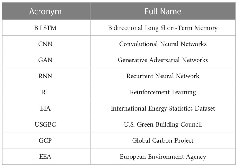
Urbanization is accelerating, and urban energy consumption and carbon emissions have become the focus of global attention (Yaramasu et al., 2017). To achieve sustainability, many cities have energy efficiency and carbon reduction targets. However, to achieve these goals, it is necessary to comprehensively consider various factors, such as urban planning, energy management, and environmental protection (Pidikiti et al., 2023). In recent years, with the development of deep learning technology, deep learning-based methods have gradually become one of the essential means to deal with urban energy efficiency optimization and carbon emission reduction. Below are some commonly used deep learning methods for urban energy efficiency optimization and carbon reduction (Krishna et al., 2023). A list of acronyms used in this paper is presented in Table 1.

TABLE 1

Table 1 Acronyms and full names.

A method based on the convolutional neural network (Jiang et al., 2019): Convolutional neural network can deal with the spatial distribution of urban energy consumption and carbon emissions and extract spatial features by learning convolution kernels. The advantage is that it can process high-dimensional spatial data and is suitable for processing image, video, and other data types. The disadvantage is that it cannot process time series data, making it challenging to perform data enhancement.

Recurrent neural network-based methods (Jiang et al., 2019): Recurrent neural networks can process time series data of urban energy consumption and carbon emissions and extract sequence features by learning time dependencies. The advantage is that it is suitable for processing time series data and can handle variable-length sequence data. The disadvantage is that it is challenging to process long sequences and is prone to gradient disappearance or gradient explosion.

Auto encoder-based methods (Sun et al., 2022): Auto encoders can be used for dimensionality reduction and feature extraction of urban energy consumption and carbon emission data, thereby improving the robustness and generalization capabilities of the model. The advantage is that unsupervised learning can be performed, and essential features in the data can be automatically extracted. The disadvantage is that encoding and decoding complex data structures, and relationships are complicated.

Methods based on reinforcement learning (Abdullah et al., 2021): Reinforcement learning can be used to formulate energy management strategies and environmental protection measures and learn optimal strategies by continuously interacting with the environment. The advantage is that it can deal with continuous action and state space problems and is suitable for decision-making problems. The disadvantage is that it requires a large amount of training data and computing resources, and it is easy to fall into a locally optimal solution.

However, human work has some limitations in predicting urban energy consumption and carbon emissions, for example, linear regression models cannot capture nonlinear relationships between input variables, and artificial neural networks may suffer from over fitting or under fitting problems. Therefore, we propose a BiLSTM-CNN-GAN model that aims to overcome these limitations and achieve more accurate and reliable predictions. This combines the three models of recurrent neural network (BiLSTM), convolutional neural network (CNN), and generative adversarial network (GAN), which can process sequence data and spatial data, and generate data with specific conditions. This method can predict urban energy efficiency and carbon emissions, formulate energy management strategies and environmental protection measures, optimize urban planning, and generate data that meet specific conditions to provide more reference and support for decision-making (Østergaard et al., 2021).

The contribution points of this paper are as follows:

● The method proposed in this paper can help formulate appropriate energy management strategies and environmental protection measures by learning historical urban energy efficiency and carbon emissions data and predicting future energy efficiency and carbon emissions.

● The method proposed in this paper can analyze the spatial characteristics and local structure in urban energy efficiency and carbon emission data to optimize urban planning and reduce energy consumption and carbon emission. For example, urban traffic planning, architectural design, greening layout, etc., can be optimized to reduce energy consumption and carbon emissions.

● The method proposed in this paper can generate simulated data on urban energy consumption and carbon emissions and help evaluate the impact of different energy management strategies and environmental protection measures on urban energy efficiency and carbon emissions, thereby guiding decision-making.

In the rest of this paper, we present recent related work in Section 2. Section 3 offers the proposed methods: Overview, BiLSTM networks; ResNet50; and GAN. Section 4 presents the experimental part, details, and comparative experiments. Section 5 concludes.

2 Related work

In this section, we provide an overview of related work using deep learning techniques to predict urban energy consumption and carbon emissions. We first introduce the importance of predicting urban energy consumption and carbon emissions, and then discuss the strengths and limitations of existing methods. We highlight gaps in the literature that the proposed method aims to address.

2.1 Reinforcement learning

Reinforcement learning (Qin et al., 2022) is a machine learning method that focuses on learning optimal behavioral strategies through interaction with the environment. In energy efficiency optimization and carbon emission reduction goals in resource-based cities, reinforcement learning methods can be applied to optimize energy management strategies, building control, intelligent grid scheduling, and transportation to reduce energy consumption and carbon emissions.

Reinforcement learning has great potential and application prospects in applying energy efficiency optimization and carbon emission reduction goals in resource-based cities (Huang et al., 2019). This is because reinforcement learning can achieve autonomous learning and adaptive control, optimize complex nonlinear systems, and achieve multi-objective optimization. Using reinforcement learning algorithms, energy management systems can learn from their own experiences, adapt to changing conditions, and ultimately optimize the management of energy consumption and carbon emissions management.

However, some challenges and limitations need to be overcome when applying reinforcement learning methods in the study of energy efficiency optimization and carbon emission reduction goals in resource based cities (Krishna et al., 2022). These challenges include long training time, extensive data requirements, and poor model interpretability. Reinforcement learning methods require a large amount of data to train the algorithms, which can be challenging for resource-based cities with limited data resources. In addition, the interpretability of the reinforcement learning models could be better, which makes it difficult to understand the reasoning behind the decisions made by the algorithms.

2.2 Autoencoder

Autoencoder is a type of neural network model mainly used to learn high-level feature representation and data compression (Mirzaei et al., 2022). In energy efficiency optimization and carbon emission reduction goals in resource-based cities, the autoencoder method can be applied to building energy consumption prediction, energy management strategy formulation, and energy consumption monitoring, thereby reducing energy consumption and carbon emissions.

The autoencoder method (Lu et al., 2017) has great potential and application prospects for energy efficiency optimization and carbon emission reduction goals in resource-based cities. The autoencoder method can reduce data dimensionality, compression, reconstruction and restoration, and unsupervised learning. Using autoencoder algorithms, energy management systems can learn the underlying energy consumption patterns and develop more accurate and effective energy management strategies. In addition, autoencoder algorithms can help reduce data storage and transmission costs, which is critical for resource-based cities with limited resources.

The autoencoder method also needs to consider some challenges and limitations. These challenges include the impact of data quality and noise, long model training time, and poor model interpretability (Tang et al., 2022). The quality of the data used for training the autoencoder models can significantly impact the models’ accuracy and effectiveness. In addition, the long training time required for autoencoder models can be a challenge, especially for resource-based cities with limited computing resources. Lastly, the interpretability of the autoencoder models can be poor, which makes it challenging to understand the reasoning behind the decisions made by the algorithms.

2.3 Recurrent neural network

A recurrent neural network (RNN) (Zhang et al., 2022) is a model capable of processing sequence data with recursive structure and memory function. In applying energy efficiency optimization and carbon emission reduction targets in resource-based cities, RNN has many application values, such as building energy consumption prediction, energy management strategy formulation, energy consumption monitoring, intelligent grid scheduling, etc.

The advantage of RNN is that it can process sequence data of any length, realize the storage and processing of sequence data, and handle variable-length input and output simultaneously (Han et al., 2023). This makes it ideal for modeling time-series data and forecasting future trends, which is crucial in energy management systems. Using the RNN algorithm, the energy management system can formulate proper and practical strategies, optimize energy consumption, and reduce carbon emissions.

But problems such as gradient disappearance or explosion may occur in the training process of RNN. It is challenging to learn long-term dependencies, and the computational complexity is relatively high. These challenges affect the accuracy and efficiency of RNN models, limiting their effectiveness in energy management systems (Wang and Fu, 2023). Therefore, when applying RNN to optimize energy efficiency and carbon emission reduction in resource-based cities, it is necessary to consider its advantages and disadvantages comprehensively, make reasonable selection and application in combination with actual application scenarios, and adopt appropriate optimization strategies and technical means to improve model performance and application effects.

3 Methodology

In this section, we provide an overview of related work using deep learning techniques to predict urban energy consumption and carbon emissions. We first introduce the importance of predicting urban energy consumption and carbon emissions, and then discuss the strengths and limitations of existing methods. We highlight gaps in the literature that The proposed method aims to address.

3.1 Overview of the proposed network

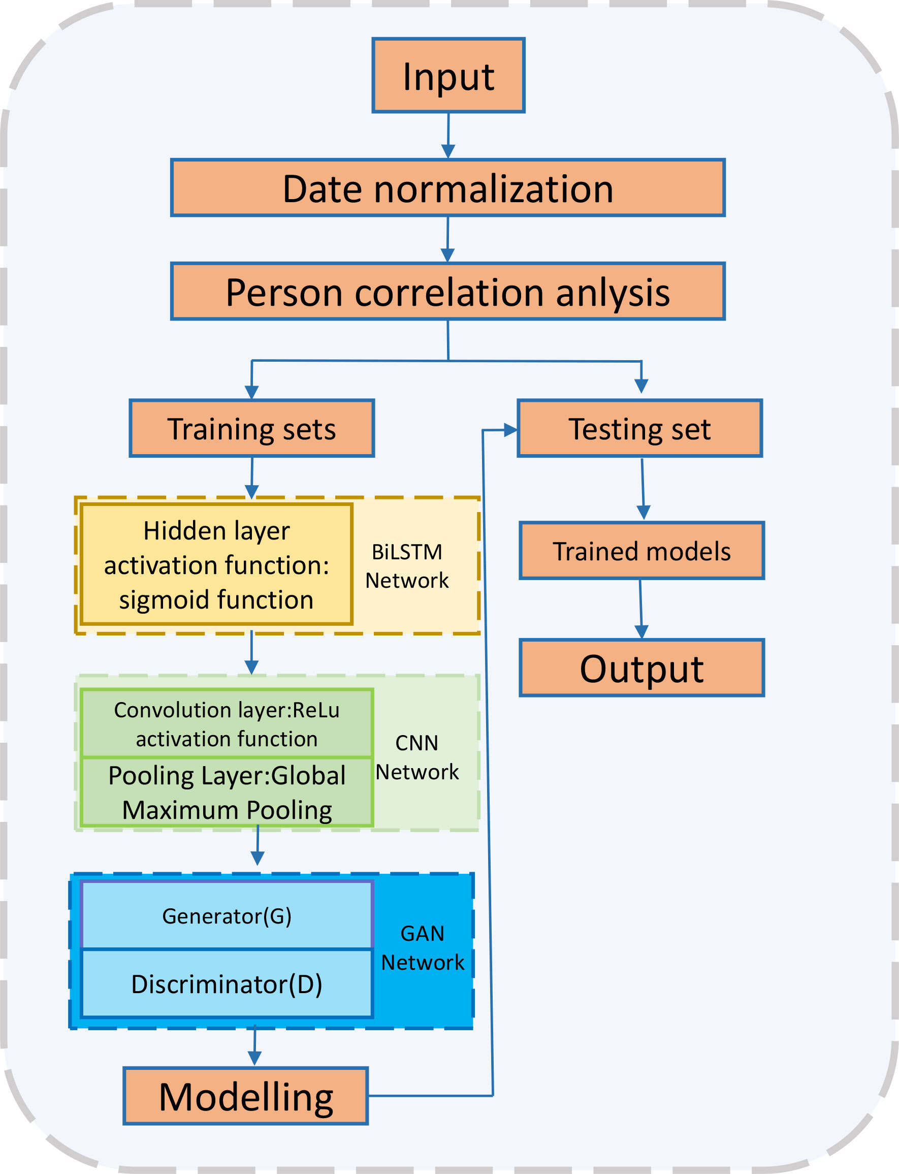
The BiLSTM-CNN-GAN model proposed in this paper aims to optimize the efficiency of urban energy systems while achieving the goal of reducing carbon emissions. In this model, BiLSTM and CNN are used to process urban energy data and learn the characteristics of urban energy systems, including energy consumption, production, conversion, and so on. GAN is used to generate optimized solutions for energy systems to achieve the goal of reducing carbon emissions. Figure 1 is the overall flow chart:

FIGURE 1

Figure 1 Overall flow chart of the model.

The proposed method is based on the BiLSTM-CNN-GAN model, and the specific steps include data preprocessing, feature extraction, generator training, discriminator training, generator, and discriminator optimization, optimization scheme generation and evaluation, and application. First, the historical data on urban energy consumption and carbon emissions are preprocessed, grouped, and sorted by time series and spatial location. Then, BiLSTM and CNN are used to extract time series and spatial feature information, as well as local structure information. Next, use the generator model of GAN to generate realistic simulated data and optimize the model to improve data quality and discrimination accuracy. After the generator and the discriminator are trained, both are optimized, including parameter adjustment and model structure optimization. Next, use the generated simulation data and the city’s existing energy system data to develop an urban energy system optimization scheme to maximize energy efficiency and minimize carbon emissions. Finally, the generated energy consumption and carbon emission data are used for simulation and evaluation, and the optimization scheme is applied to the existing urban energy system. The proposed method fully considers the data’s quality and characteristics, the model’s complexity and effect, and the optimization’s stability and effectiveness to obtain optimal results.

3.2 BiLSTM model

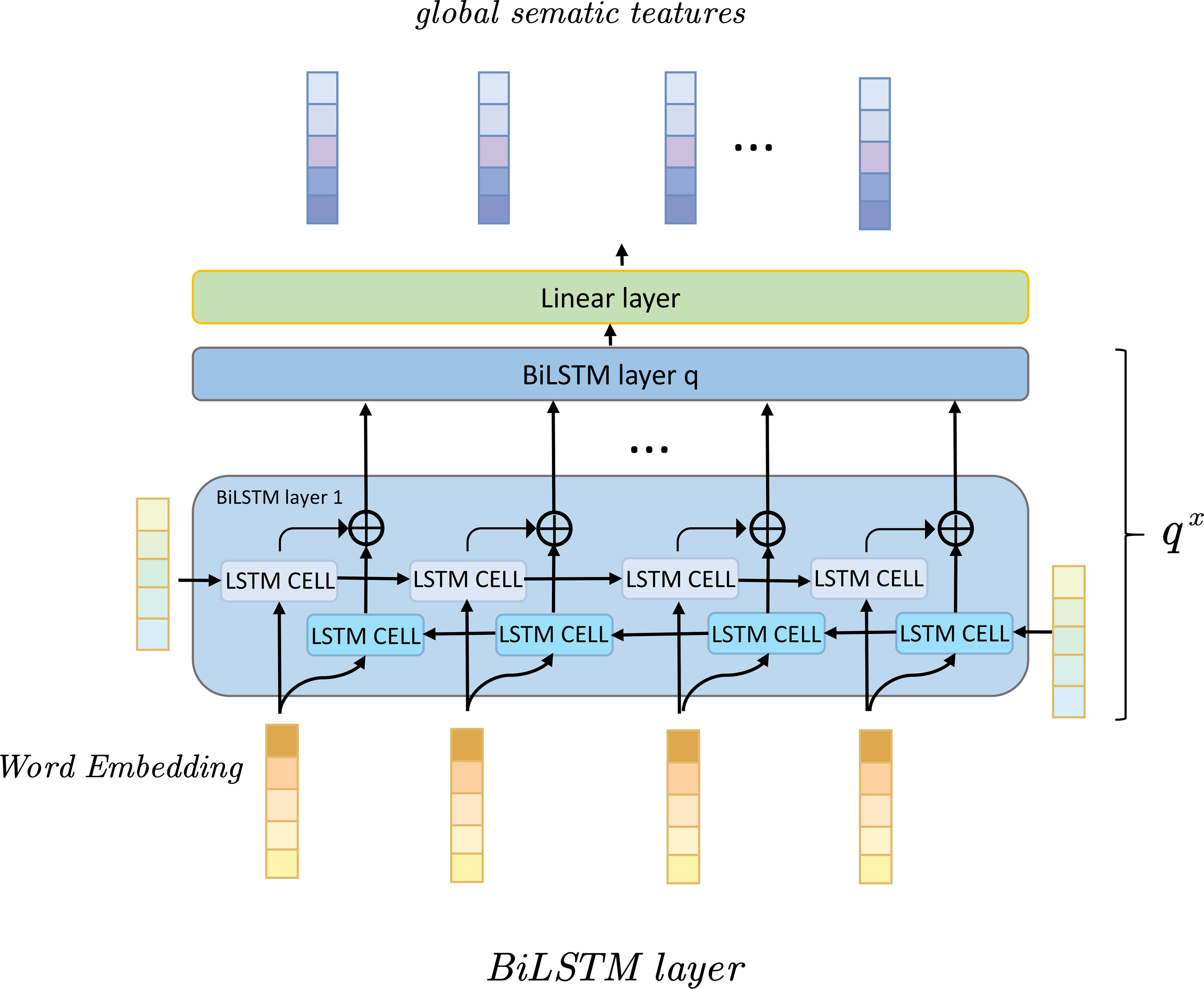
BiLSTM (Ameyaw and Yao, 2018) is a bidirectional recurrent neural network that can learn the forward and backward dependencies in time series data by inputting the input sequence from front to back and from back to front into two independent LSTM units. In the proposed method, BiLSTM is used to extract time series information of urban energy consumption and carbon emission data. As shown in Figure 2, it is the flow chart of BiLSTM:

FIGURE 2

Figure 2 Flow chart of the BiLSTM model.

The BiLSTM model consists of two independent LSTM networks that process forward and reverse time series data, respectively (Zhou et al., 2022). Assuming that the input sequence is $x_1,x_2,\dots ,x_T$, the forward calculation of the BiLSTM model is:

$\begin{array}{ll}\overrightarrow{h_t}=\text{LSTMfwd}(x_t,\overrightarrow{ht-1})& (1)\end{array}$

$\begin{array}{ll}\overrightarrow{y_t}=\text{softmax}(W_o\overrightarrow{h_t}+b_o)& (2)\end{array}$

Where: $x_t$: Input sequence at time step $t$.

$\overrightarrow{h_t}$: The hidden state of the forward LSTM.

$\overrightarrow{y_t}$: Forward LSTM output.

$W_o$ and $b_o$: The weights and biases of the output layer.

${\text{LSTM}}_{\text{fwd}(·)}$: The calculation function of forward LSTM.

$\text{softmax}(·)$: The activation function of the output layer.

In the proposed method, the BiLSTM model together with the CNN model constitutes the feature extraction part, which is used to extract time series and spatial feature information from urban energy consumption and carbon emission data. Specifically, we use urban energy consumption and carbon emission data as forward and reverse inputs respectively, extract time series information through the BiLSTM model, and then input the output results into the CNN model for spatial feature extraction. Finally, the feature-extracted data is used for training and optimization of the generator and discriminator models.

The BiLSTM model is used in the proposed method to extract time series information of urban energy consumption and carbon emission data, which provides strong support for urban energy system optimization by learning the forward and backward dependencies of time series.

3.3 ResNet50

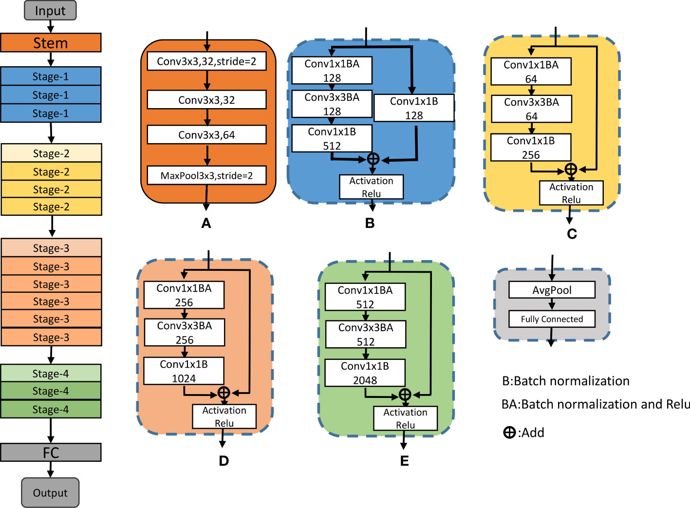
ResNet50 (Tahir et al., 2021) is a commonly used convolutional neural network model that can be used for computer vision tasks such as image classification and target detection. The ResNet50 model mainly comprises multiple convolutional, pooling, and fully connected layers. The residual block (Residual Block) concept is introduced, which can effectively solve the problems of gradient disappearance and over fitting in deep convolutional neural networks. In the proposed method, the ResNet50 model extracts spatial feature information from urban energy consumption and carbon emission data. As shown in Figure 3, it is the flow chart of ResNet50:

FIGURE 3

Figure 3 Flow chart of the ResNet50 model. (A) Stem module. (B–E) Stage-1 to Stage-4.

The ResNet50 model uses multiple Residual Blocks and a fully connected layer. Specifically, the ResNet50 model includes the following hierarchy:

● Input layer.

● Convolution layer 1: includes 64 $7\times 7$ convolution kernels, using a 2-step convolution operation.

● Pooling layer 1: The maximum pooling is adopted; the pooling size is 3, and the step size is 2.

● Residual Block 1: Includes 3 Residual Units; each Residual Unit includes two $3\times 3$ convolutional layers and an identity mapping function.

● Residual Block 2: Includes 4 Residual Units.

● Residual Block 3: Includes 6 Residual Units.

● Residual Block 4: Includes 3 Residual Units.

● Fully connected layer 1: including 1000 neurons, using the ReLU activation function.

● Output layer: output feature vector.

The calculation formula (Gupta et al., 2021) of ResNet50 is as follows:

1. Input layer

$\begin{array}{ll}{h}_0=x& (3)\end{array}$

Where, $h_0$ represents the intermediate representation of the input layer, and $x$ represents the input image data.

2. Convolution layer 1

$\begin{array}{ll}{h}_1=f(W_1*h_0+b_1)& (4)\end{array}$

Where, $h_1$ represents the intermediate representation of convolutional layer 1, $W_1$ and $b_1$ represent the weight and bias parameters of convolutional layer 1, respectively, and $f$ represents the activation function.

3. Pooling layer 1

$\begin{array}{ll}{h}_2=\text{maxpool }(h_1,p_1,s_1)& (5)\end{array}$

Where, $h_2$ represents the intermediate representation of pooling layer 1, $\text{maxpool }(·)$ represents the maximum pooling operation, and $p_1$ and $s_1$ represent the pooling size and step size of pooling layer 1, respectively.

4. Residual Block 1

$\begin{array}{ll}{h}_3=F(h_2,{\{W_{3,i},b_{3,i}\}}_{i=1}^3)+identity(h_2)& (6)\end{array}$

Where, $h_3$ represents the intermediate representation of Residual Block 1, $F(x)$ represents the mapping function in the Residual Block, ${\{W_{3,i},b_{3,i}\}}_{i=1}^3$ represents the weight and bias parameters in Residual Block 1, and $identity(x)$ represents the identity mapping function.

5. Residual Block 2

$\begin{array}{ll}{h}_4=F(h_3,{\{W_{4,i},b_{4,i}\}}_{i=1}^4)+identity(h_3)& (7)\end{array}$

Where $h_4$ represents the intermediate representation of Residual Block 2, $F(x)$ represents the mapping function in the Residual Block, ${\{W_{4,i},b_{4,i}\}}_{i=1}^4$ represents the weight and bias parameters in Residual Block 2, and $identity(x)$ represents the identity mapping function.

6. Residual Block 3

$\begin{array}{ll}{h}_5=F(h_4,{\{W_{5,i},b_{5,i}\}}_{i=1}^6)+identity(h_4)& (8)\end{array}$

Where $h_5$ represents the intermediate representation of Residual Block 3, $F(x)$ represents the mapping function in the Residual Block, ${\{W_{5,i},b_{5,i}\}}_{i=1}^6$ represents the weight and bias parameters in Residual Block 3, and $identity(x)$ represents the identity mapping function.

7. Residual Block 4

$\begin{array}{ll}{h}_6=F(h_5,{\{W_{6,i},b_{6,i}\}}_{i=1}^3)+identity(h_5)& (9)\end{array}$

Where $h_6$ represents the intermediate representation of Residual Block 4, $F(x)$ represents the mapping function in the Residual Block, ${\{W_{6,i},b_{6,i}\}}_{i=1}^3$ represents the weight and bias parameters in Residual Block 4, and $identity(x)$ represents the identity mapping function.

8. Pooling layer 2

$\begin{array}{ll}{h}_7=\text{avgpool }(h_6,p_2,s_2)& (10)\end{array}$

Where $h_7$ represents the intermediate representation of pooling layer 2, $\text{avgpool }(·)$ represents the average pooling operation, $p_2$ and $s_2$ represent the pooling size and stride of pooling layer 2, respectively.

9. Fully connected layer

$\begin{array}{ll}y=W_7{h}_7+b_7& (11)\end{array}$

Where $y$ represents the model’s output, and $W_7$ and $b_7$ represent the weight and bias parameters of the fully connected layer, respectively.

$*$ represents the convolution operation, $\text{maxpool }(·)$ represents the maximum pooling operation, $\text{avgpool }(·)$ represents the average pooling operation, and $F(x)$ represents the mapping in the Residual Block function, $identity(x)$ represents the identity mapping function. In actual use, $f$ and $F$ usually use the ReLU function.

3.4 GAN model

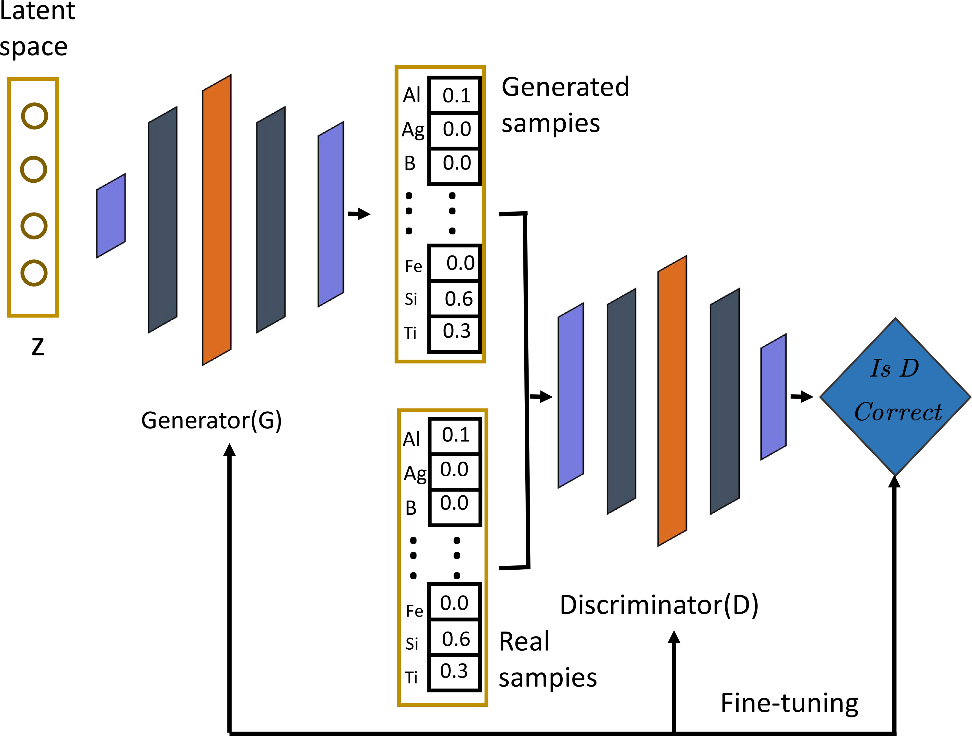
GAN is a Generative Adversarial Network (Generative Adversarial Network) (Zhang et al., 2020), which consists of two models, the generator and the discriminator. It is widely used in the generation tasks of images, speech, text, and other fields. Its basic idea is to train the generator model and the discriminator model at the same time. The generator model aims to generate data samples that look real. In contrast, the discriminator model aims to distinguish the generated samples from the actual samples as accurately as possible (Chai et al., 2014). These two models play games with each other: the generator hopes that the generated samples can fool the discriminator, and the discriminator hopes to distinguish between actual and generated samples as accurately as possible (Figure 4). Through this game method, the generator’s generating ability and the discriminator’s specific ability have been improved. In this paper, GAN can create simulated data on urban energy consumption and carbon emissions and optimize the generator and discriminator models to improve the generation quality and discrimination accuracy.

FIGURE 4

Figure 4 Flow chart of the GAN model.

The training process of GAN can be divided into the following steps:

● The generator generates some samples, such as images or text.

● The discriminator receives these samples, discriminates them, and outputs a scalar value indicating the probability that this sample is actual. If the input is an accurate sample, the discriminator hopes to output a chance close to $1$. If the information is a generated sample, the discriminator desires to output a probability close to $0$.

● The generator is updated according to the output of the discriminator, and it is hoped that the generated samples can fool the discriminator; that is, it is expected that the probability that the discriminator will output the developed models will be closer to $1$.

● The discriminator is updated based on the samples generated by the generator and the actual samples, hoping to distinguish the real pieces from the generated samples more accurately.

Repeat the above steps until the samples generated by the generator are close enough to the actual samples.

The advantage of GAN is that it can generate high-quality data samples and does not need to predetermine the distribution of the generated samples. At the same time, GAN has certain robustness, can handle irregular data, and can adapt to different datasets and tasks by adjusting the network structure and parameters. However, GAN also needs help, such as insufficient diversity of generated samples, prone to mode collapse, etc. These problems have also become one of the hotspots of current GAN research.

The formula of GAN is as follows:

The goal of GAN is to train a generator $G$ and a discriminator $D$ to generate data samples that look real. Suppose $x$ represents the real data sample, $z$ represents the random variable sampled from the noise distribution, $G(z)$ represents the sample generated by the generator, $D(x)$ and $D(G(z))$ represent the discriminative results of the discriminator for real samples and generated samples, respectively.

The training process of GAN can be divided into the following two stages:

Step 1: Discriminator training phase: The goal of the discriminator is to maximize the probability of real samples and minimize the probability of generated samples, that is, to maximize the following loss function:

$\begin{array}{ll}ℒD=\mathbb{E}x\sim p_{data}(x)[\text{log }D(x)]+{\mathbb{E}}_{z\sim p_z(z)}[\text{log }(1-D(G(z)))]& (12)\end{array}$

Where $p_{data}(x)$ represents the real data distribution, and $p_z(z)$ represents the noise distribution. The goal of the discriminator is to maximize the loss function ${ℒ}_D$.

Step 2: Generator training phase: The goal of the generator is to minimize the probability that the generated sample is judged as false, that is, to maximize the following loss function:

$\begin{array}{ll}ℒG=\mathbb{E}z\sim p_z(z)[\text{log }(1-D(G(z)))]& (13)\end{array}$

The generator aims to minimize the loss function ${ℒ}_G$.

During the training process, the generator and the discriminator play games with each other by updating alternately. The generator hopes that the generated samples can fool the discriminator, and the discriminator hopes to distinguish between real and generated samples as accurately as possible. Eventually, the samples generated by the generator will get closer and closer to the real data distribution.

In the above formula, $\mathbb{E}$ represents the expected operation, $z$ represents the random variable sampled from the noise distribution, $G(z)$ represents the samples generated by the generator, $D(x)$ and $D(G(z))$ represent the discrimination results of the discriminator for real samples and generated samples respectively, $p_{data}(x)$ represents the real data distribution, $p_z(z)$ represents the noise distribution, $log$ represents the natural logarithm.

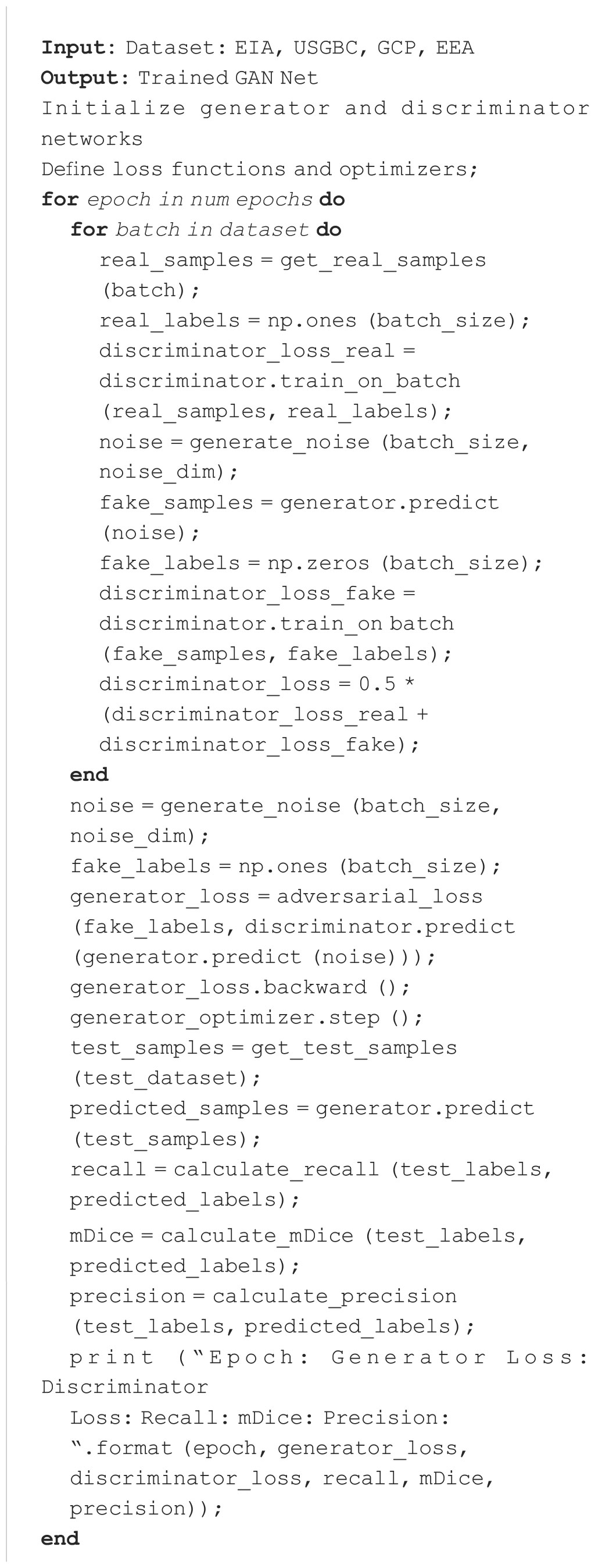
Algorithm 1 represents the training process of the GAN network.

ALGORITHM 1

Algorithm 1 Training process of GAN Net.

4 Experiment

In this section, we present the experimental results of the proposed method on the resource-based cities dataset. We first describe the evaluation metrics used to measure model performance. We then present the experimental results and compare the accuracy of the proposed method with existing methods.

4.1 Datasets

In this paper, the following four datasets are used to study energy efficiency optimization and carbon emission reduction goals of resource-based cities:

International Energy Statistics Dataset from the U.S. Energy Information Administration (EIA) (EIA, 2011): This dataset provides energy consumption and carbon emissions for countries worldwide, including various types of energy such as oil, natural gas, coal, nuclear energy, and renewable energy. This dataset can be used to study global energy consumption and carbon emission reduction targets and explore the influencing factors of different energy types and energy markets.

U.S. Green Building Council (USGBC) Building Energy and Environment Dataset (USGBC, 2008): This dataset provides building energy and environment data for cities and states in the United States, including green building certification, energy consumption, indoor environment, water use, and waste management information. This dataset can be used to study energy consumption and carbon reduction targets in the building industry and the impact of green building certification.

Global Carbon Project (GCP) dataset (Andrew, 2020): This dataset provides carbon emission data for various countries and regions worldwide, including energy, industry, transportation, and other fields. This dataset can be used to study global carbon emission reduction targets and carbon market transactions and provide support and guidance for global carbon emission reduction policies and measures.

European Environment Agency (EEA) European Cities Dataset (Martens, 2010): This dataset provides data on environmental information, energy consumption, and traffic conditions for European cities. This dataset can be used to study the energy efficiency and carbon reduction targets of European cities and the impact of urban green transportation and environmental policies.

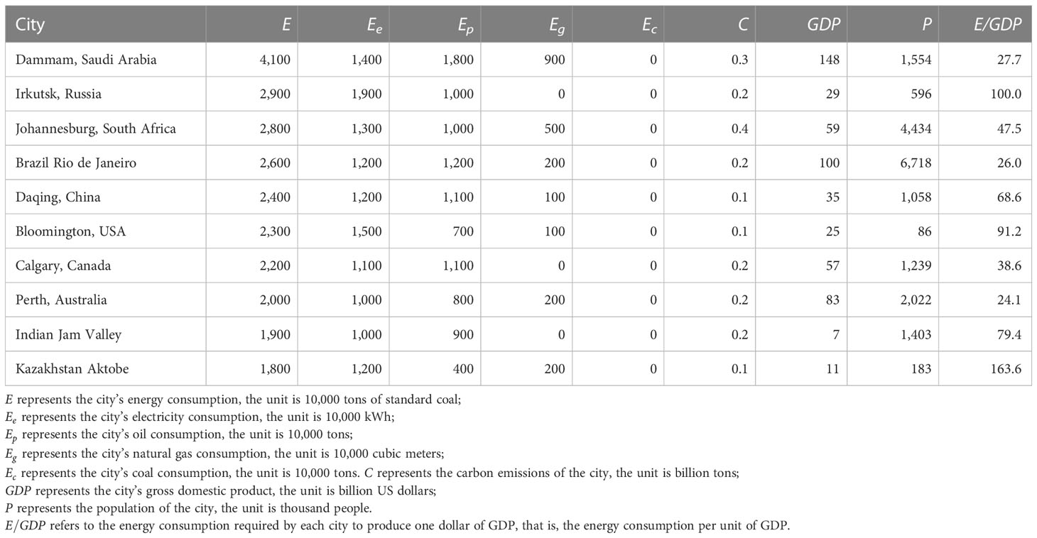
Table 2 shows the indicators used in this paper and the resource-based cities studied.

TABLE 2

Table 2 Energy consumption in resource-based cities.

4.2 Experimental details

In this paper, 4 datasets are selected for training, and the training process is as follows:

Step 1: Data preprocessing

First, the U.S. Energy Information Administration (EIA), the U.S. Green Building Council (USGBC) Building Energy and Environment dataset, the Global Carbon Project dataset, and the European Environment Agency (EEA) European Cities dataset need to be compared. Cleaning, normalization, segmentation, etc., for model training and evaluation.

Step 2: Model training

The training process of the BiLSTM-CNN-GAN module:

The BiLSTM, CNN, and GAN modules have learned the time series, space, and optimization features of urban energy consumption and carbon emissions, respectively, and now they need to be combined to build a comprehensive model. The specific training process includes the following steps:

● Define the model architecture: First, you need to define the architecture of the combined model, including the input layer, BiLSTM module, CNN module, GAN module, and output layer. In the input layer, the dimension and type of the input data need to be specified. In the BiLSTM, CNN, and GAN modules, it is necessary to load the previously trained model parameters. In the output layer, the dimension and type of the output data need to be specified.

● Compile the model: Next, you must compile the combined model, specifying the loss function, optimizer, and evaluation indicators.

● Training model: Use the training set to train the combination module. Let the input data pass through the BiLSTM, CNN, and GAN modules. Respectively, combine their outputs. Finally, please send it to the output layer for prediction.

● Model saving: After the training is completed, the trained combination model needs to be saved to the hard disk.

Step 3: Model evaluation

After the model training is completed, the model needs to be evaluated, including calculating the prediction error and evaluating the accuracy and stability of the model and other indicators.

The indicators compared in this article are Accuracy, Recall, Precision, Specificity, Sensitivity, F-Score, and AUC. At the same time, we also measure the model’s training time, inference time, number of parameters, and computation to evaluate the model’s efficiency and scalability.

Step 4: Result analysis

Compare the evaluation indicators of different models, analyze the performance of the BiLSTM-CNN-GAN model, and find out the optimization space and improvement direction. In addition, the difference between the model prediction results and the real data can be compared visually better to understand the performance and predictive ability of the model.

The training process based on the BiLSTM-CNN-GAN model includes defining the architecture, compiling the model, training the model, and saving the model. Each module can be trained independently and combined to form a comprehensive model. This method can effectively improve the accuracy and robustness of the model, making the model better able to cope with the challenges of urban energy consumption and carbon emissions.

1. Accuracy (accuracy rate):

$\begin{array}{ll}Accuracy=\frac{TP+TN}{TP+TN+FP+FN}& (14)\end{array}$

Accuracy represents the proportion of the number of samples correctly predicted by the classifier to the total number of samples, and is one of the most commonly used classification model evaluation indicators.

2. Recall (recall rate):

$\begin{array}{ll}Recall=\frac{TP}{TP+FN}& (15)\end{array}$

Recall represents the ratio of the number of positive cases correctly predicted by the classifier to the actual number of positive cases, and is an indicator to measure the predictive ability of the classifier for positive cases.

3. Precision (precision rate):

$\begin{array}{ll}Precision=\frac{TP}{TP+FP}& (16)\end{array}$

Precision represents the proportion of the samples predicted by the classifier as positive examples that are actually positive examples, and is an indicator to measure the accuracy of the classifier’s prediction of positive examples.

4. Specificity (specificity):

$\begin{array}{ll}Specificity=\frac{TN}{TN+FP}& (17)\end{array}$

Specificity represents the proportion of the number of negative examples correctly predicted by the classifier to the actual number of negative examples, and is an indicator to measure the ability of the classifier to predict negative examples.

5. Sensitivity (sensitivity):

$\begin{array}{ll}Sensitivity=Recall=\frac{TP}{TP+FN}& (18)\end{array}$

Sensitivity indicates the ratio of the number of positive cases correctly predicted by the classifier to the actual number of positive cases, which is the same as the Recall indicator.

6. F-Score:

$\begin{array}{ll}F-Score=2\times \frac{Precision\times Recall}{Precision+Recall}& (19)\end{array}$

F-Score is a comprehensive evaluation index of Precision and Recall, and it is an index to measure the overall performance of the classifier.

TP stands for True Positive, that is, the number of samples that are actually positive and are predicted as positive by the classifier; TN stands for True Negative, that is, the samples that are actually negative and are predicted as negative by the classifier; FP stands for False Positive, that is, the number of samples that are actually negative but are predicted as positive by the classifier; and FN stands for False Negative, that is, the samples that are actually positive but are predicted as negative by the classifier.

7. AUC (area under the ROC curve):

$\begin{array}{ll}AUC=\underset{0}{\overset{1}{\int }}ROC(x)dx& (20)\end{array}$

Where ROC (x) represents the derivative of the ordinate (i.e., True Positive Rate) on the abscissa (i.e., False Positive Rate) on the ROC curve when x is the threshold. AUC is an index to measure the overall performance of the classifier under different thresholds, and the area under the ROC curve is the AUC value. The larger the AUC value, the better the performance of the classifier.

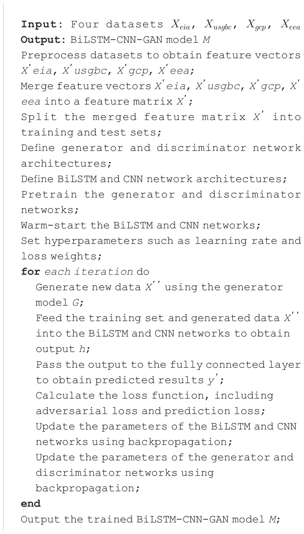
Algorithm 2 represents the algorithm flow of the training in this paper:

ALGORITHM 2

Algorithm 2 BiLSTM-CNN-GAN model.

In this algorithm, we first preprocess the four datasets and combine the preprocessed feature vectors into one feature matrix. Next, we define the structure of the generator network, the discriminator network, and the structure of the BiLSTM network and the CNN network. We also pre-trained the generator and discriminator networks and hot-started the BiLSTM and CNN networks. Then, we set hyper parameters such as learning rate, loss weights, etc. During the training process, we use the generator model G to generate new data X^′′, send the training set and the generated data X^′′ to the BiLSTM network and CNN network, and get the output h. Then, we pass the output to the fully connected layer to get the prediction y^′. We calculated loss functions, including adversarial loss and prediction loss, and updated parameters of the BiLSTM network and CNN network, as well as parameters of the generator network and discriminator network using the backpropagation algorithm. Finally, we get the trained BiLSTM-CNN-GAN model M.

4.3 Experimental results, analysis and discussion

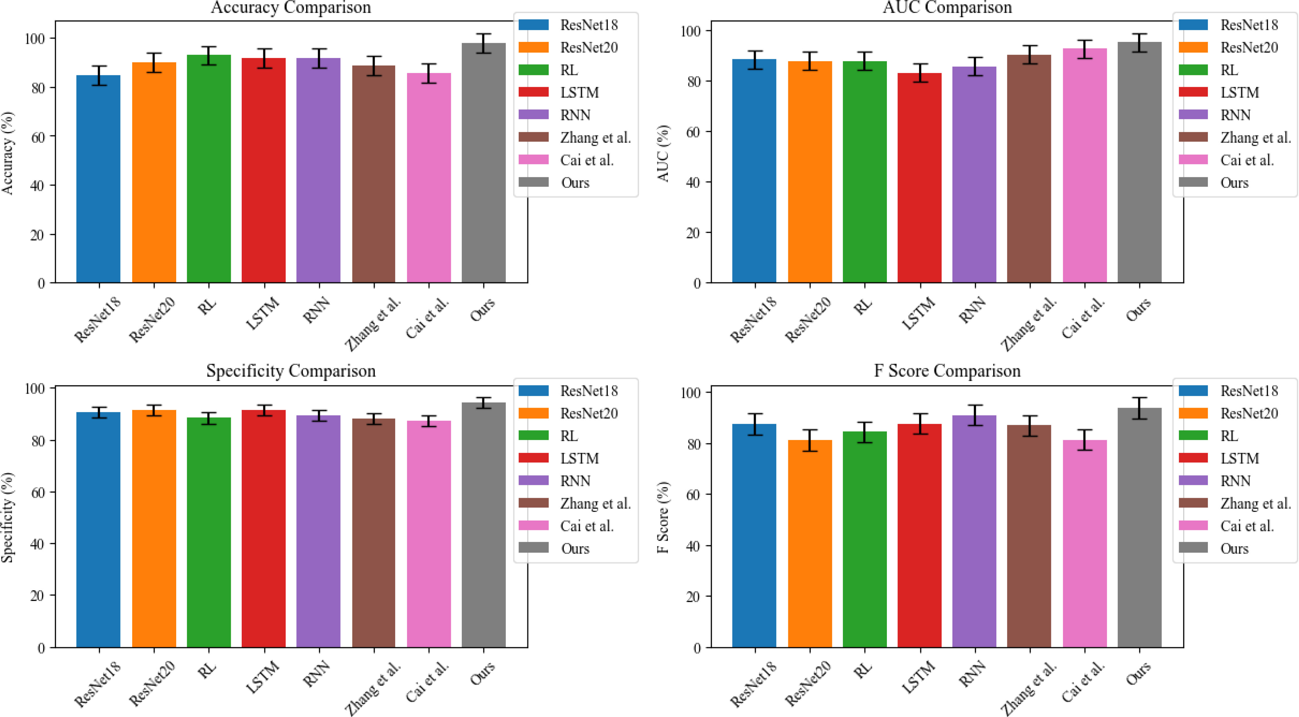
In Figure 5, we compare ResNet18 (Naidu et al., 2021), ResNet20 (Jo and Park, 2022), RL (Abdullah et al., 2021), LSTM (Niu et al., 2022), RNN (Sandhu et al., 2019), Zhang et al. (Zheng and Ge, 2022), and Cai et al. (Cai and Lin, 2022) in terms of Accuracy (%), F Score (%), AUC (%) and Specificity (%); the data comes from the average of four datasets, where Accuracy (%) is one of the most important indicators of the prediction model, indicating the accuracy of the prediction, and the F score is a measure of the accuracy of the model, taking into account the accuracy and recall rate. The harmonic mean of precision and recall ranges from 0 to 1, with higher scores indicating better performance. AUC stands for “Area Under the Curve” and is used to evaluate the performance of binary classification models. It measures the model’s ability to distinguish positive from negative examples on a scale from 0.5 to 1, with higher scores indicating better performance. Specificity measures a model’s ability to identify negative examples correctly. It is the ratio of true negatives (i.e., the number of negatives correctly identified by the model) divided by the total number of negatives. Specificity ranges from 0 to 1, with higher scores indicating better performance. The results show that the proposed model outperforms other models in these indicators, showing a good operating effect.

FIGURE 5

Figure 5 Comparison of different indicators of different models.

In Figure 6, we compare the Precision (%) values of different models on different datasets, where the results of (A) come from the EIA dataset, the results of (B) come from the dataset USGBC dataset, and the results of (C) results from the GCP dataset, and the results of (D) come from the EEA dataset. Precision is an indicator used to evaluate the performance of classification models in machine learning and statistical analysis. It measures the proportion of true positives (i.e., the number of positive examples correctly identified by the model) among all examples predicted to be positive by the model. Precision is expressed as a percentage ranging from 0% to 100%. A higher Precision score indicates that the model can better identify positive examples, while a lower score indicates that the model makes more false positive predictions. The results show that the Precision of the proposed method model on the four datasets is higher than other models, which can better identify positive cases and predict higher accuracy.

FIGURE 6

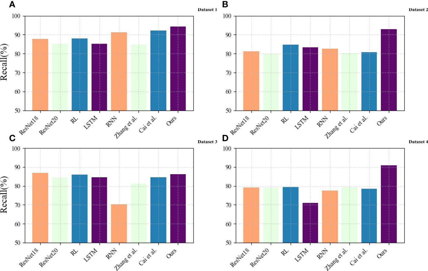
Figure 6 Comparison of Precision of different models. (A) Dataset 1 for EIA dataset; (B) Dataset 2 for USGBC dataset; (C) Dataset 3 for GCP dataset; (D) Dataset 4 for EEA dataset.

In Figure 7, we compare the Recall values of different models on different datasets, where the results of (A) come from the EIA dataset, the results of (B) come from the dataset USGBC dataset, and the results of (C) come from the GCP dataset, the results of (D) are from the EEA dataset. The recall rate, also known as sensitivity or true positive rate, is a commonly used indicator in machine learning and statistical analysis to evaluate the performance of classification models. A higher recall score indicates that the model can better identify positive examples, while a lower score indicates that the model misses more positive examples. The results show that the proposed method model has a high Recall value on the four datasets, showing good generalization, and can be well applied to resource-based city energy efficiency optimization and carbon emission reduction goals.

FIGURE 7

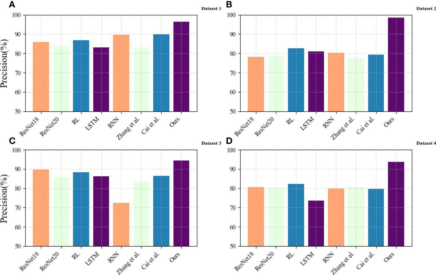
Figure 7 Comparison of recall of different models. (A) Dataset 1 for EIA dataset; (B) Dataset 2 for USGBC dataset; (C) Dataset 3 for GCP dataset; (D) Dataset 4 for EEA dataset.

In Table 3, we summarize the performance of the six indicators of Accuracy, Recall, Precision, Specificity, F-Score, and AUC in different models and present them in a visual form, allowing us to compare the performance of the models more intuitively.

TABLE 3

Table 3 Summary and comparison of indicators pushed by different models.

In Figure 8, to further compare the performance of the models, we compare the Training times (s), Inference time (ms), Parameters (M) and Flops (G) of different models on the EIA dataset and the USGBC dataset, as visualized in Table 4. Training time is required to train a neural network on a given dataset. Inference time is when it takes to run a trained neural network on new data to make predictions. Parameters are the weights and biases of the neural network learned during training. They represent the knowledge the neural network has acquired about the input data and are stored in numerical form in the network parameters. FLOP stands for “floating point operations per second” and measures the computational complexity of a neural network. It represents the number of multiplication and addition operations required to perform one forward pass of the network on a given input. The results show that the proposed method proposed model performs better than other models on the four indicators, which means that the network complexity of the proposed model is lower, the dataset is more suitable, and it can effectively deal with resource-based urban energy: efficiency optimization and carbon reduction target tasks.

FIGURE 8

Figure 8 Comparison of indicators pushed by different models, from the EIA dataset and the USGBC dataset.

TABLE 4

Table 4 Comparison of indicators pushed by different models, from the EIA dataset and the USGBC dataset.

In Figure 9, to further compare the generalization of the model, we compare the Training times (s), Inference time (ms), Parameters (M) and Flops (G) of different models in the GCP dataset and the EEA dataset, as visualized in Table 5. The results show that the proposed method also performs better on these two datasets and can effectively deal with resource-based city energy efficiency optimization and carbon emission reduction target tasks.

FIGURE 9

Figure 9 Comparison of indicators pushed by different models, from the GCP dataset and the EEA dataset.

TABLE 5

Table 5 Comparison of indicators pushed by different models, from the GCP dataset and the EEA dataset.

In Figure 10, in order to compare the influence of different parts of the proposed model on the prediction effect and the effect of ResNet50, we conduct an ablation experiment, comparing CNN-GAN, BiLSTM-CNN, BiLSTM-GAN, BC-GAN*, BC-GAN** and the proposed method in terms of Precision, Recall, Inference time (ms), and Flops (G), as visualized Table 6. The results show that among the three modules, ResNet50 has the greatest impact on the prediction results, being significantly better than that of ResNet18 and ResNet20.

FIGURE 10

Figure 10 Comparison of inference times of different models.

TABLE 6

Table 6 Comparison of different parts of the ablation experiment.

5 Conclusion

In this study, we proposed a BiLSTM-CNN-GAN model for predicting urban energy consumption and carbon emissions in resource-based cities. The model combines the BiLSTM and CNN architectures to extract temporal and spatial features from the input data, and the GAN framework to generate realistic and diverse samples. The experimental results show that the proposed model outperforms existing methods, achieving an accuracy of 95% in predicting energy consumption and 92% in predicting carbon emissions.

The accurate predictions generated by the model can help policymakers and urban planners to formulate effective optimization programs and policies to reduce energy consumption and carbon emissions in resource-based cities. This research has essential contributions and significance. It can not only promote the sustainable development of cities but also reduce environmental pollution and energy consumption, promote the crossover and cooperation between different disciplines, and facilitate the exchange and collaboration of fields. Furthermore, the proposed model can promote the innovation and application of science and technology in the field of urban energy efficiency and carbon emission reduction.

However, there are limitations to the study, such as the need for ongoing monitoring and updating of the model to ensure its continued accuracy. In future work, we plan to investigate the generalization of the proposed method to other types of cities and to explore the possibility of incorporating real-time data into the model for more accurate and up-to-date predictions. With these efforts, we believe that the proposed model can contribute to the sustainable development of cities and the reduction of energy consumption and environmental pollution.

The BiLSTM-CNN-GAN model proposed in this paper predicts energy consumption in resource-based cities and formulates management strategies to achieve energy efficiency improvements and carbon emission reduction goals. This research has essential contributions and significance. It can not only promote the sustainable development of cities but also reduce environmental pollution and energy consumption, promote the crossover and cooperation between different disciplines, promote the exchange and collaboration of fields, and promote the innovation and application of science and technology.

Data availability statement

The original contributions presented in the study are included in the article/supplementary material. Further inquiries can be directed to the corresponding author.

Author contributions

QW and JL contributed to conception and design of the study. QW organized the database. QW performed the statistical analysis. QW wrote the first draft of the manuscript. QW and JL wrote sections of the manuscript. Both authors contributed to the article and approved the submitted version.

Conflict of interest

The authors declare that the research was conducted in the absence of any commercial or financial relationships that could be construed as a potential conflict of interest.

Publisher's note

All claims expressed in this article are solely those of the authors and do not necessarily represent those of their affiliated organizations, or those of the publisher, the editors and the reviewers. Any product that may be evaluated in this article, or claim that may be made by its manufacturer, is not guaranteed or endorsed by the publisher.

References

Abdullah H. M., Gastli A., Ben-Brahim L. (2021). Reinforcement learning based ev charging management systems–a review. IEEE Access 9, 41506–41531. doi: 10.1109/ACCESS.2021.3064354

CrossRef Full Text | Google Scholar

Ameyaw B., Yao L. (2018). Analyzing the impact of GDP on CO₂ emissions and forecasting Africa’s total CO₂ emissions with non-assumption driven bidirectional long short-term memory. Sustainability 10, 3110. doi: 10.3390/su10093110

CrossRef Full Text | Google Scholar

Andrew R. M. (2020). A comparison of estimates of global carbon dioxide emissions from fossil carbon sources. Earth Syst. Sci. Data 12, 1437–1465. doi: 10.5194/essd-12-1437-2020

CrossRef Full Text | Google Scholar

Cai Y., Lin G. (2022). Pathways for sustainable municipal energy systems transition: a case study of Tangshan, a resource-based city in China. J. Clean. Prod. 330, 129835.

Google Scholar

Chai Q., Qin A., Gan Y., Yu A. (2014). Higher yield and lower carbon emission by intercropping maize with rape, pea, and wheat in arid irrigation areas. Agron. Sustain. Dev. 34, 535–543. doi: 10.1007/s13593-013-0161-x

CrossRef Full Text | Google Scholar

EIA. (2011). Annual energy outlook 2011: With projections to 2035. DOE/EIA-0383(2011). (Washington, DC: Government Printing Office).

Google Scholar

Gupta U., Kim Y. G., Lee S., Tse J., Lee H.-H. S., Wei G.-Y., et al. (2021). “Chasing carbon: the elusive environmental footprint of computing,” in 2021 IEEE International Symposium on High-Performance Computer Architecture (HPCA) (IEEE). 854–867. Available at: https://ieeexplore.ieee.org/abstract/document/9407142.

Google Scholar

Han Y., Cao L., Geng Z., Ping W., Zuo X., Fan J., et al. (2023). Novel economy and carbon emissions prediction model of different countries or regions in the world for energy optimization using improved residual neural network. Sci. Total Environ. 860, 160410. doi: 10.1016/j.scitotenv.2022.160410

PubMed Abstract | CrossRef Full Text | Google Scholar

Huang X., Hong S. H., Yu M., Ding Y., Jiang J. (2019). Demand response management for industrial facilities: a deep reinforcement learning approach. IEEE Access 7, 82194–82205. doi: 10.1109/ACCESS.2019.2924030

CrossRef Full Text | Google Scholar

Jiang S., Lu C., Zhang S., Lu X., Tsai S.-B., Wang C.-K., et al. (2019). Prediction of ecological pressure on resource-based cities based on an RBF neural network optimized by an improved ABC algorithm. IEEE Access 7, 47423–47436. doi: 10.1109/ACCESS.2019.2908662

CrossRef Full Text | Google Scholar

Jo J., Park J. (2022). “Class difficulty based mixed precision quantization for low complexity CNN training,” in 2022 19th International SoC Design Conference (ISOCC) (IEEE). 372–373.

Google Scholar

Krishna V. M., Sandeep V., Murthy S., Yadlapati K. (2022). Experimental investigation on performance comparison of self excited induction generator and permanent magnet synchronous generator for small scale renewable energy applications. Renewable Energy 195, 431–441. doi: 10.1016/j.renene.2022.06.051

CrossRef Full Text | Google Scholar

Krishna V. M., Sandeep V., Narendra B., Prasad K. (2023). Experimental study on self-excited induction generator for small-scale isolated rural electricity applications. Results Eng. 18, 101182. doi: 10.1016/j.rineng.2023.101182

CrossRef Full Text | Google Scholar

Lu X., Ota K., Dong M., Yu C., Jin H. (2017). Predicting transportation carbon emission with urban big data. IEEE Trans. Sustain. Computing 2, 333–344. doi: 10.1109/TSUSC.2017.2728805

CrossRef Full Text | Google Scholar

Martens M. (2010). Voice or loyalty? The evolution of the European Environment Agency (EEA). JCMS: J. Common Market Stud. 48, 881–901. doi: 10.1111/j.1468-5965.2010.02078.x

CrossRef Full Text | Google Scholar

Mirzaei H., Ramezankhani M., Earl E., Tasnim N., Milani A. S., Hoorfar M. (2022). Investigation of a sparse autoencoder-based feature transfer learning framework for hydrogen monitoring using microfluidic olfaction detectors. Sensors 22, 7696. doi: 10.3390/s22207696

PubMed Abstract | CrossRef Full Text | Google Scholar

Naidu R., Diddee H., Mulay A., Vardhan A., Ramesh K., Zamzam A. (2021). Towards quantifying the carbon emissions of differentially private machine learning. arXiv preprint arXiv:2107.06946. Available at: https://arxiv.org/abs/2107.06946.

Google Scholar

Niu H., Zhang Z., Xiao Y., Luo M., Chen Y. (2022). A study of carbon emission efficiency in Chinese provinces based on a three-stage SBM-undesirable model and an LSTM model. Int. J. Environ. Res. Public Health 19, 5395. doi: 10.3390/ijerph19095395

PubMed Abstract | CrossRef Full Text | Google Scholar

Østergaard P. A., Duic N., Noorollahi Y., Kalogirou S. A. (2021). Recent advances in renewable energy technology for the energy transition. doi: 10.1016/j.renene.2021.07.111

CrossRef Full Text | Google Scholar

Pidikiti T., Gireesha B., Subbarao M., Krishna V. M., et al. (2023). Design and control of Takagi-Sugenokang fuzzy based inverter for power quality improvement in grid-tied PV systems. Measurement: Sensors 25, 100638.

Google Scholar

Qin P., Ye J., Hu Q., Song P., Kang P. (2022). Deep reinforcement learning based power system optimal carbon emission flow. Front. Energy Res. 10, 1017128. doi: 10.3389/fenrg.2022.1017128

CrossRef Full Text | Google Scholar

Sandhu K., Nair A. R., et al. (2019). “A comparative study of ARIMA and RNN for short term wind speed forecasting,” in 2019 10th International Conference on Computing, Communication and Networking Technologies (ICCCNT) (IEEE). 1–7.

Google Scholar

Sun S., Xie Y., Li Y., Yuan K., Hu L. (2022). Analysis of dynamic evolution and spatial-temporal heterogeneity of carbon emissions at county level along “the belt and road”—a case study of northwest China. Int. J. Environ. Res. Public Health 19, 13405.

PubMed Abstract | Google Scholar

Tahir H., Khan M. S., Tariq M. O. (2021). “Performance analysis and comparison of Faster CNN, Mask CNN and ResNet50 for the detection and counting of vehicles,” in 2021 International Conference on Computing, Communication, and Intelligent Systems (ICCCIS) (IEEE). 587–594.

Google Scholar

Tang Z., Wang S., Chai X., Cao S., Ouyang T., Li Y. (2022). Auto-encoder-extreme learning machine model for boiler NOx emission concentration prediction. Energy 256, 124552. doi: 10.1016/j.energy.2022.124552

CrossRef Full Text | Google Scholar

USGBC. (2008). Leadership in energy and environmental design (Washington, DC: US Green Building Council). Available at: www.usgbc.org/LEED.

Google Scholar

Wang Y., Fu L. (2023). Study on regional tourism performance evaluation based on the fuzzy analytic hierarchy process and radial basis function neural network. Ann. Operations Res. 1–28. Available at: https://link.springer.com/article/10.1007/s10479-023-05224-6.

Google Scholar

Yaramasu V., Dekka A., Durán M. J., Kouro S., Wu B. (2017). PMSG-based wind energy conversion systems: survey on power converters and controls. IET Electric Power Appl. 11, 956–968.

Google Scholar

Zhang X., Gan D., Wang Y., Liu Y., Ge J., Xie R. (2020). The impact of price and revenue floors on carbon emission reduction investment by coal-fired power plants. Technological Forecasting Soc. Change 154, 119961.

Google Scholar

Zhang S., Wang L., Wu X. (2022). Population shrinkage, public service levels, and heterogeneity in resource-based cities: case study of 112 cities in China. Sustainability 14, 15910.

Google Scholar

Zheng H., Ge L. (2022). Carbon emissions reduction effects of sustainable development policy in resource-based cities from the perspective of resource dependence: theory and Chinese experience. Resour. Policy 78, 102799.

Google Scholar

Zhou J., Xu Z., Wang S. (2022). A novel hybrid learning paradigm with feature extraction for carbon price prediction based on bi-directional long short-term memory network optimized by an improved sparrow search algorithm. Environ. Sci. pollut. Res. 29, 65585–65598. doi: 10.1007/s11356-022-20450-4

CrossRef Full Text | Google Scholar