- 1School of Ecology and Nature Conservation, Beijing Forestry University, Beijing, China
- 2National Park (Nature Protected Area) Development Center, National Forestry and Grassland Administration, Beijing, China
- 3Department of Biological and Environmental Science, College of Agricultural, Life and Natural Sciences, Alabama A&M University, Normal, AL, United States
Climate and land-use changes and their interactions have a profound effect on biodiversity, especially in biodiverse areas such as Southeast Asia (SEA) where aggregations of endemic species are widespread. To increase the effectiveness of biodiversity protection, it is crucial to understand the effect of climate and land-use changes on biodiversity. In the present study, we predicted future land-use changes based on a Cellular automaton Markov chain model (CA-MARKOV), and took Galliformes species as an example to assess the impact of climate and land-use changes on the effectiveness of protected areas in SEA. In addition, we used an ensemble of species distribution models (SDMs) to assess the potential habitats and their dynamics of 62 Galliformes species currently and in the 2070s. Our results showed that climate and land-use changes would reduce the suitable habitats of these Galliformes species. Among them, 22 or 31 species would migrate upward because of a decrease in habitat suitability at lower elevations caused by climate and land-use changes, while other 40 or 30 species were predicted to migrate downward because of land use changes under two dispersal scenarios. These changes would expand the area with low and high diversity, but there would be a mismatch between the current protected areas (PAs) and future suitable habitats with high diversity. In order to effectively ensure biodiversity protection and conserve 30% of the planet by 2030, our findings suggest that we should establish new PAs or adjust the range of PAs based on the impact of climate and land-use changes.
1 Introduction
Global warming and anthropogenic land-use changes are considered to have irreversible effects on biodiversity (Jetz et al., 2007; Pearce-Higgins et al., 2017), including suitable habitat range reduction (Brambilla et al., 2020), population decline (Powers and Jetz, 2019) and genetic diversity loss (Hu et al., 2021). Climate change usually affects the species distribution of mammals (Brodie, 2016; Hidasi-Neto et al., 2019), birds (Jetz et al., 2007; Lehikoinen and Virkkala, 2016), lizards (Jiang et al., 2023), etc. by reducing habitat suitability. Besides, it may aggravate the extinction risk of species (Urban, 2015; Manes et al., 2021). For instance, Sekercioglu et al. (2007) have predicted that 400–550 landbirds will be extinct as a result of future changes by 2100. Protected areas (PAs) are considered as refuges for species, and can mitigate the impact of climate change on species (Shen et al., 2015; Michalak et al., 2018). However, recent studies have suggested that current PAs will be challenged by future climate change (Kyprioti et al., 2021; Salvadeo et al., 2021), and may fail to provide enough space for species. Therefore, an accurate prediction of future species distribution is necessary for managers to develop policies that can mitigate the impact of future climate change on species.
Moreover, landscape patterns also need to be considered in the prediction of future species distribution. A previous study has predicted that 1700 species of mammals, birds and amphibians may lose suitable habitats due to land-use changes between 2015 and 2070 (Powers and Jetz, 2019). Current land-use changes such as road construction, urbanization and transforming natural habitats into farmland can influence habitat connectivity (Krauss et al., 2010; Hansen et al., 2013; Wilson et al., 2015; Tang et al., 2020). Habitats changed by human activity were hereinafter referred to as “altered habitats”. Although several species of birds have been demonstrated to inhabit altered habitats or edges between natural and altered habitats (Kark et al., 2007; Møller et al., 2012; Carlen et al., 2021), most wild species have suffered habitat loss due to land-use changes (Powers and Jetz, 2019; Shahabuddin et al., 2021).
In addition, climate and land-use changes are widely observed to have a combined influence on species (Côté et al., 2016; Keshtkar and Voigt, 2016; Symes et al., 2018; Northrup et al., 2019; Bühne et al., 2021). The interactions between climate and land-use changes are predicted to have more negative impacts on species than any single factor (Symes et al., 2018; Northrup et al., 2019; Bühne et al., 2021). The increased quantity of manmade landscapes is attributed to declining natural habitats, increased CO2 emissions and accelerated global warming (Kucuker et al., 2015). Habitat loss has especially disastrous consequences for forest-dependent species (Gaüzère et al., 2020; Hülber et al., 2020), and climate change further aggravates the impact of land-use changes on species with specific geographic ranges and migration abilities (Jetz et al., 2007; Brodie, 2016; Dai et al., 2021). Ignoring the combined influence of climate and land-use changes on biodiversity may result in an underestimation of the situation, whereas examining the combined impacts of these variables can provide a better prediction for species conservation (Titeux et al., 2016; Northrup et al., 2019).
Southeast Asia (SEA) is a world-famous biodiversity hotspot with abundant forest resource. However, people have been transforming forest into farmland and towns for survival and economic development, which led to the loss and fragmentation of forests (Estoque et al., 2019). These undoubtedly exacerbated the loss of biodiversity, and it seems unstoppable (Sodhi et al., 2010). Galliformes is an important component of biodiversity and they have a high value in economy and culture for residents of SEA. Therefore, they were often regarded as the main targets of hunters (Savini et al., 2021). According to the records, SEA encompassed the habitat range of 77 Galliformes species, and about 27% of them are at risk of extinction (IUCN, 2023). Unfavorable forest transformation always had negative effects on Galliformes species that inhabit forest landscapes (Grainger et al., 2018; Savini et al., 2021), and it directly changed land-use patterns and indirectly accelerates global warming (Bos et al., 2020). These changes will aggravate the survival pressure of Galliformes. Protected areas were powerful tools for protecting wildlife and their habitat (UNEP-WCMC, 2022), Previous study showed that intensities of human interference in protected areas of SEA are greater than that of other regions in the world (Geldmann et al., 2019), and protected areas could not protect the intact forests effectively in SEA (Potapov et al., 2017). Galliformes were often taken as indicators of habitat conditions (Bagaria et al., 2021), and because of their extinction risk, they also were used to evaluate the conservation status of SEA (Grainger et al., 2018). Therefore, evaluating how the Galliformes species inhabiting forest landscapes respond to climate and land-use changes is crucial to assess the conservation status of SEA and formulate management measures. Here, we assessed the potential habitats of Galliformes species and their variations under climate and land-use changes in SEA. We aimed to: 1) evaluate the impact of climate and land-use changes on the distribution of Galliformes species; 2) predict the changes in species diversity; and 3) identify conservation gaps and provide suggestions for future protection.
2 Materials and methods
2.1 Study area and species data collection
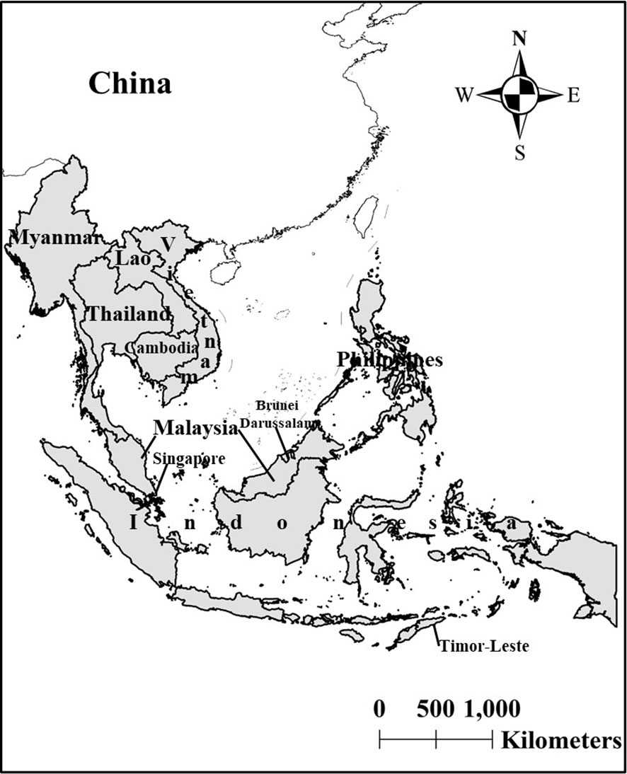
SEA encompassed countries (Figure 1) including the Republic of the Union of Myanmar (MMR), Thailand (THA), Brunei Darussalam (BRN), Lao People’s Democratic Republic (LAO), Cambodia (KHM), the Socialist Republic of Vietnam (VNM), Malaysia (MYS), the Republic of Singapore (SGP), the Republic of Indonesia (IDN), the Republic of the Philippines (PHL) and the Democratic Republic of Timor-Leste (TMP) (Grainger et al., 2018; Savini et al., 2021).
We identified 77 native Galliformes species distributed in SEA and verified species whether is extinct or introduced in 11 countries according to IUCN Red List, also collected the occurrence data of them from Global Biodiversity Information Facility (GBIF.org, 2021), ebirds (https://ebird.org/) and inaturalist (https://www.inaturalist.org/) from 2000 to 2020. To develop the effectiveness of these data (Meyer et al., 2016; Stropp et al., 2016), we excluded points that were not displayed in A Checklist on the Classification and Distribution of the Birds of the World (Second Edition) (Zheng, 2021), and deleted the repetitive and default (NA value) points. Specifically, red junglefowl (Gallus gallus) was not considered in our study due to the possibility of misidentification between wild and domestic individuals during observation. We excluded species with less than 10 individuals. As a result, we obtained a total of 7701 points of 62 species for further analysis (Appendix. Table B.1).
2.2 Environmental variables
2.2.1 Climatic variables
Climate change can alter the climate niche of species (Selwood and Zimmer, 2020). To describe the potential effect of future climate change on Galliformes species in SEA, we compared the species distribution areas of Galliformes species between current and future climate conditions. We downloaded 19 bioclimatic variables from WorldClim 2.1 (at 1 km resolution; https://www.worldclim.org/), and they were used to represent the current climate conditions. These 19 bioclimatic variables represented annual trends (e.g., mean annual temperature and annual precipitation), seasonality (e.g., annual range in temperature and precipitation) and extreme or limiting environmental factors (e.g., temperature in the coldest and warmest months, and precipitation during the wet and dry quarters) (Fick, 2017), and were also related to the distribution of Galliformes species (Johnsgard, 1999). We also downloaded these 19 bioclimatic variables during 2061–2080 (the 2070s), and they were used to represent the future climate conditions, which covered three Shared Socioeconomic Pathways (SSP) and the Representative Concentration Pathways (RCP), including SSP126, SSP370 and SSP585. SSP126 was the combination of SSP1 and RCP 2.6, representing a low level of greenhouse gas emissions; SSP370 was the combination of SSP3 and RCP 7.0, representing a medium level of greenhouse gas emissions; and SSP585 was the combination of SSP5 and RCP 8.5, representing a high level of greenhouse gas emissions. Climatic datasets were obtained using the Beijing Climate Center Climate System Model (BCC-CSM2-MR) based on the Coupled Model Intercomparison Project (CMIP6).
2.2.2 Projection of land use and land cover changes
The Cellular automaton Markov chain model (CA-MARKOV) was used to evaluate the land use and land cover change (LULCC) from 2020 to 2080. This model combines CA method and the Markov chain model, and is widely used to predict effectively spatiotemporal changes in LULCC (Halmy et al., 2015). The CA-MARKOV model predicts future changes by quantifying the changes in LULCC between two periods (Mansour et al., 2022). First, we obtained the land cover data for 2000, 2010 and 2020 from the European Space Agency (at 300m resolution; https://cds.climate.copernicus.eu/). Next, we used the Markov chain model to calculate the transition probability and the transition area matrixes from to 2000 to 2010. Then, we used the CA-MARKOV method to test the spatial changes in cell condition and predict the spatial changes in 2020, and generated the prediction map (we refer to this as “2020p” hereinafter). The Kappa index was used to compare the similarity between 2020 and 2020p. The greater the value of the Kappa index, the more accurate the prediction (Gidey et al., 2017). We further predicted the LULCC in the 2070s (Powers and Jetz, 2019). The model processes are as follows:
where S(t)/S(t+1) represents the land use status at time t and t+1, while is the transition probability matrix in a state, representing the possibility of converting from current states i to another state j at time n; Range of is from 0 to 1, and the higher the value, the higher transition possibility.
2.2.3 Other environmental variables
Other environmental variables were used in our model including Topographic Position Index (TPI), slope and aspect. We collected the Digital Elevation Model (DEM) from SRTM (at 30m resolution; https://srtm.csi.cgiar.org). Slope and aspect were extracted from DEM by ArcGIS 10.6. The neighborhood of TPI adopted the rectangle (both of width and height are 3 pixels), and the calculation formula of TPI is as follows:
where represents the elevation of a point; represents the mean elevation of areas around this point. We kept these variables stable in future analysis.
2.3 Data analysis
2.3.1 Spatial resolution of environmental variables
All variables were in raster format, and we resampled them to 1 km resolution under GCS_WGS_1984. Variance Inflation Factor (VIF) was used to deal with the collinearity of environmental variables. The variables with VIF values > 10 were excluded from the analysis.
2.3.2 Species distribution model formulation process
Species distribution models (SDMs) are widely used to predict a species’ current and future distribution and habitat occupancy (Phillips et al., 2006; Jones-Farrand et al., 2011; Dai et al., 2021). Previous studies have shown that the predictions or projections from a single SDM may face challenges, and combining multiple SDMs (the ensemble approach) can increase the credibility of the model output (Araujo and New, 2007; Jones-Farrand et al., 2011; Kindt, 2018). RF and Maxent have been proved to have strong prediction ability (Phillips et al., 2006; Prasad et al., 2006). We assembled random forest (RF) and maximum entropy (Maxent) to predict the suitable habitat using the “sdm” package in R v.4.0.3 (Naimi and Araújo, 2016). We created a data object with species spatial points (the longitude and latitude) and predictors (retained environmental variables). The spatial points were presence-only data, and predictors were raster layers with the same spatial resolution, extent, and dimensions. In general, the absence data can be confirmed when there is sufficient evidence, but it is difficult to achieve this for living animals (Lobo and Tognelli, 2011). Therefore, we set 1000 random background points to obtain the pseudo-absence points in the same research area. Two SDMs were run as follows: 1) we randomly selected 70% of the species points for training each model, while the remaining 30% of species points were used for testing the performance of each model; 2) 10-fold cross-validation were performed to evaluate the model (Sill and Dawson, 2021). 3) The accuracy of SDMs was evaluated by the area under curve (AUC) of the receiver operating characteristic (ROC) curve; 4) Mean of the relative importance of variables was calculated based on AUC; 5) Suitable habitats of the prediction of two SDMs were assembled based on a weighted averaging that was weighted by the AUC statistic. We then used the output of fitting to project into 2070s.
2.3.3 Dispersal scenarios
Considering the dispersal behavior of species under future, we set two scenarios to identify the species suitable habitats (Feeley and Silman, 2010a), First, we assumed the Galliformes can dispersal to all potential habitat as “perfect dispersal scenarios”. Secondly, we assumed Gallidormes have the limited dispersal abilities and created a ~111 Km buffer as “limited dispersal scenarios”(Namkhan et al., 2022).
2.3.4 Changes in distribution
To understand the ecological impacts of climate change and LULCC on the distribution of Galliformes, we converted the prediction of SDMs into a binary variable (suitable or unsuitable) map by adopting the average logistic threshold value of maximum training sensitivity plus specificity. And suitable habitat losses and gains were calculated by current and future binary map. Mann–Whitney U test (variables did not pass the test for homogeneity of variance) was adopted to compare the difference in vertical distribution of species between current and future scenarios. Judgment criteria for changes in vertical distribution were shown in Appendix Table A.1. We overlapped future suitable habitat of 62 Galliformes species and used Natural breaks methods to classified them into four diversity levels (low, general, median and high) based on the number of species. Finally, we overlapped the future binary maps and the PAs that were downloaded from the Protected Planet database (https://www.protectedplanet.net/en) to identify the gaps in the current protection areas.
3 Results
3.1 Model performance
The AUC values of each SDM were greater than 0.70, indicating good predictive ability of the SDMs (Appendix Figure A.1). There were no difference in predictive ability between Maxent and RF (P >0.05). The value of Kappa for the projection by CA-MARKOV was 0.828, suggesting better predictive ability for land-use changes. The CA-MARKOV model predicted that the area of urban area, cropland, shrubland and grassland would significantly increase, while that of forest and water would decrease in the 2070s (Appendix Table.A.2). Variables retained in 62 SDMs were shown in Appendix Table B.2. Land use and precipitation of warmest quarter (Bio18) were the main factors affecting the habitat distribution of Galliformes in SEA (Appendix Figure A.2).
3.2 Suitable habitats of Galliformes under future conditions
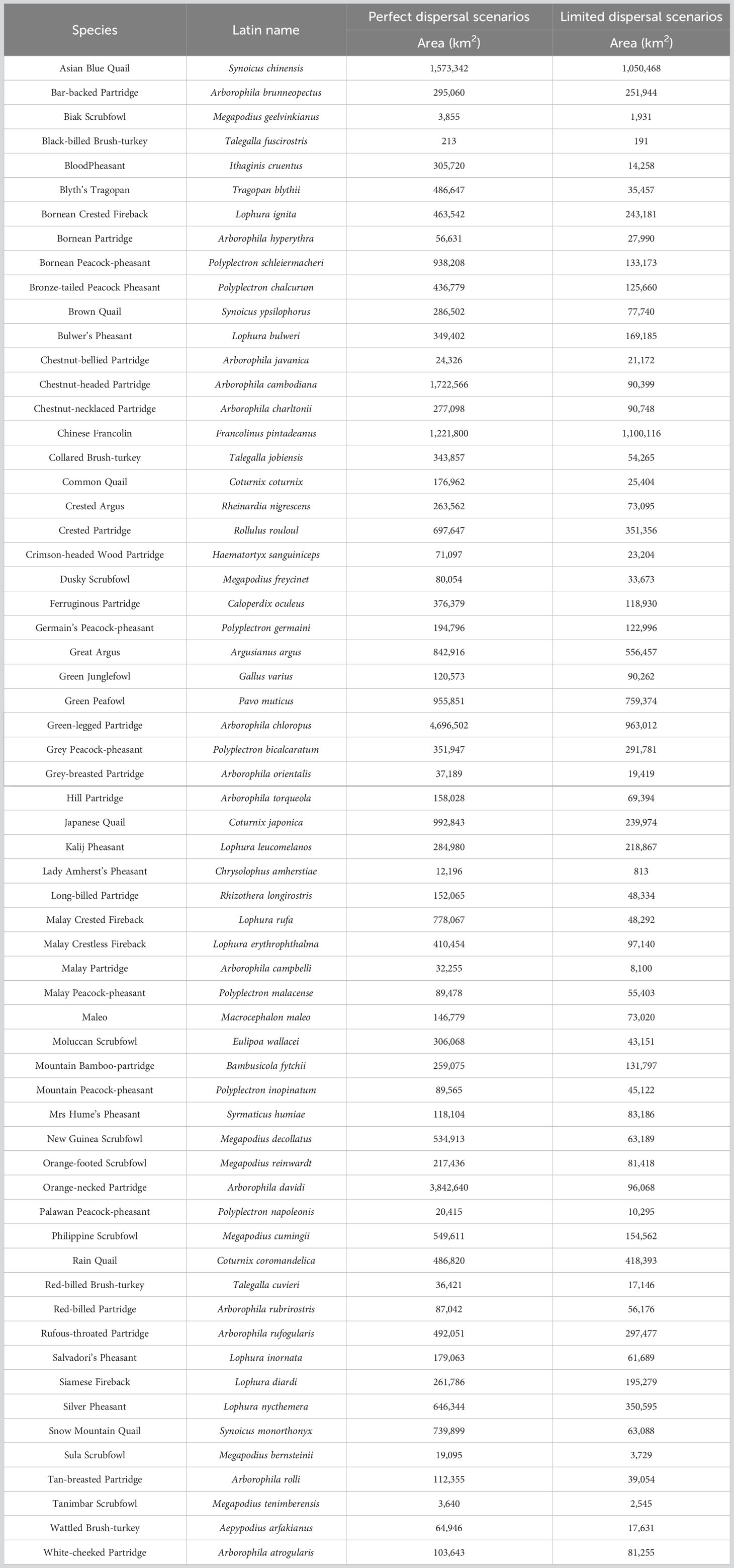
Currently, the suitable habitat area for 62 Galliformes species ranged from 213 km2 to 4,696,502 km2 under perfect dispersal scenarios, and ranged from 191 km2 to 1,100,116 km2 under limited dispersal scenarios (Table 1). At perfect dispersal scenarios, SDMs showed that the suitable habitat area for 53 species would decrease under three future scenarios, while that for other 9 species would increase (Figure 2A). There were differences in proportion of habitat gain and loss between countries, but no differences in proportion of habitat gain or loss between future scenarios (Figure 3). Laos showed a significantly higher proportion of habitat gain than Malaysia, Myanmar, Thailand, Vietnam, Indonesia and Philippines. Brunei, EastTimor and Singapore had a significantly higher proportion of habitat gain than Indonesia and Philippines (Figure 3A). And Singapore exhibited a higher proportion of habitat loss than other countries (Figure 3B).
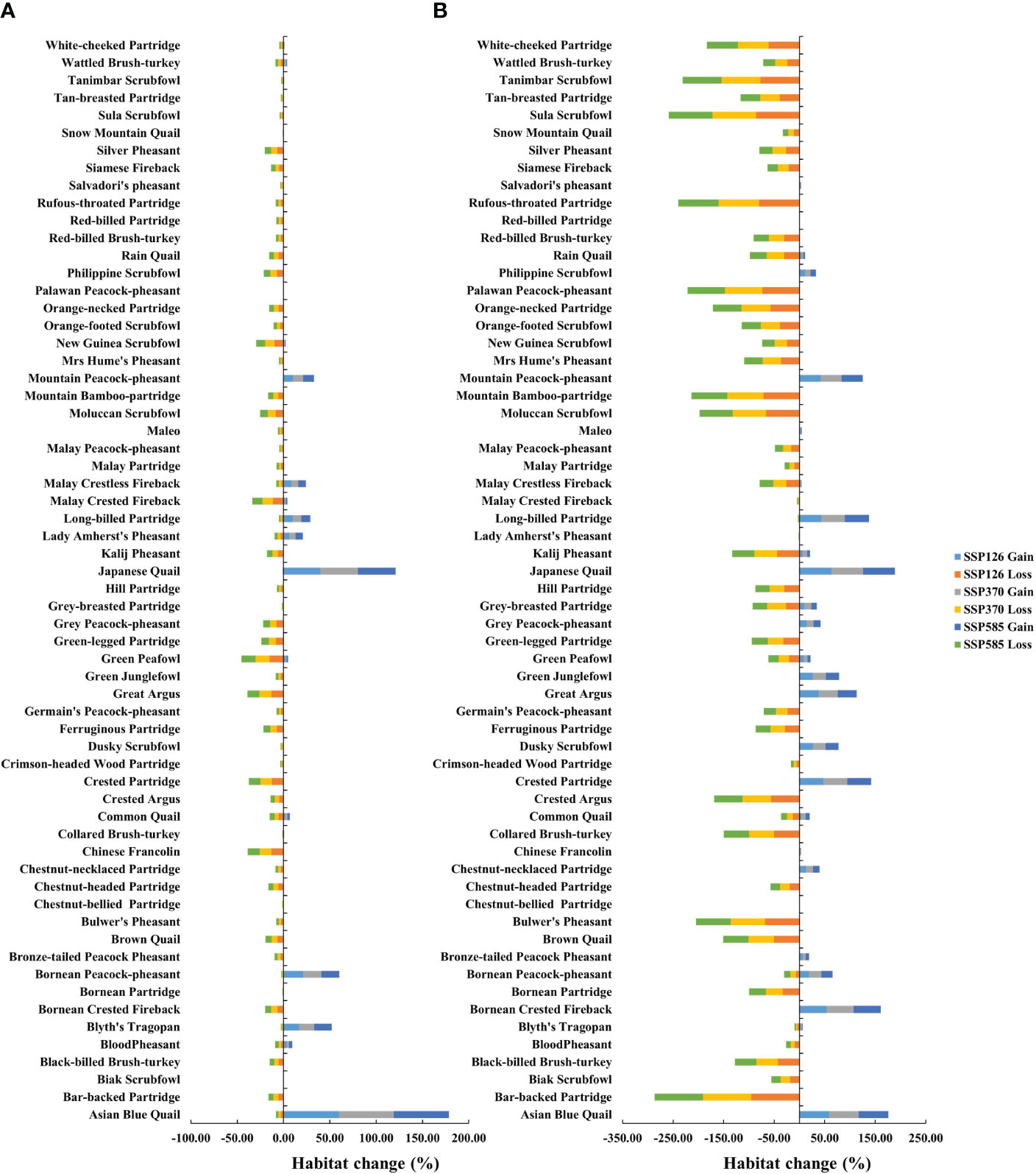
Figure 2 Proportion of habitat change under future scenarios. (A) Perfect dispersal scenarios; (B) Limited dispersal scenarios.

Figure 3 The difference in changes in suitable habitat between countries. (A) Proportion of habitat gain under perfect dispersal scenarios; (B) Proportion of habitat loss under perfect dispersal scenarios; (C) Proportion of habitat gain under limited dispersal scenarios; (D) Proportion of habitat loss under limited dispersal scenarios.
At limited dispersal scenarios, SDMs showed that the suitable habitat area for 43 species would decrease under three future scenarios, while that for other 19 species would increase (Figure 2B). There were also differences in proportion of habitat gain and loss between countries, but no differences in proportion of habitat gain or loss between future scenarios (Figure 3). Brunei showed a higher proportion of habitat gain than other countries (Figure 3C). Cambodia, Laos and Vietnam exhibited a higher proportion of habitat loss than other countries (Figure 3D).
3.3 Vertical distribution of Galliformes under future conditions
There were differences in the elevation of potential habitats between current and future scenarios. At perfect dispersal scenarios, 22 species would move upward in the future, because of habitat gain at higher elevations (Table 2). Other 40 species would move downward in the future, because of habitat gain at lower elevations or habitats loss at higher elevations (Table 2). At limited dispersal scenarios, 31 species would move upward in the future, because of habitat gain at higher elevations (Table 3). Other 30 species would move downward in the future, because of habitat gain at lower elevations or habitats loss at higher elevations (Table 3).
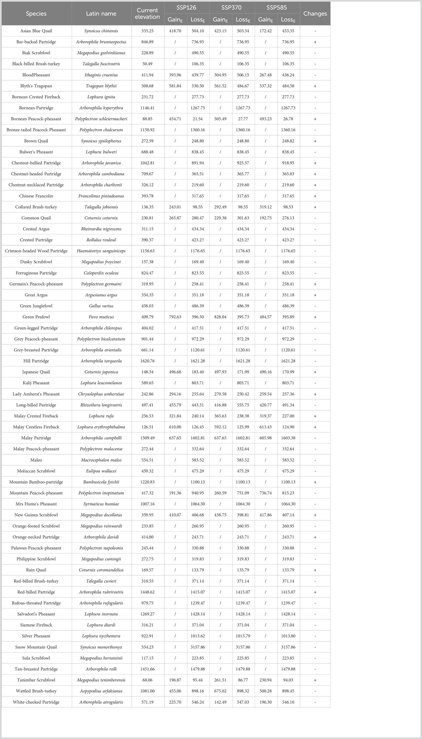
Table 2 Changes in elevation between current and future scenarios under perfect dispersal scenarios.
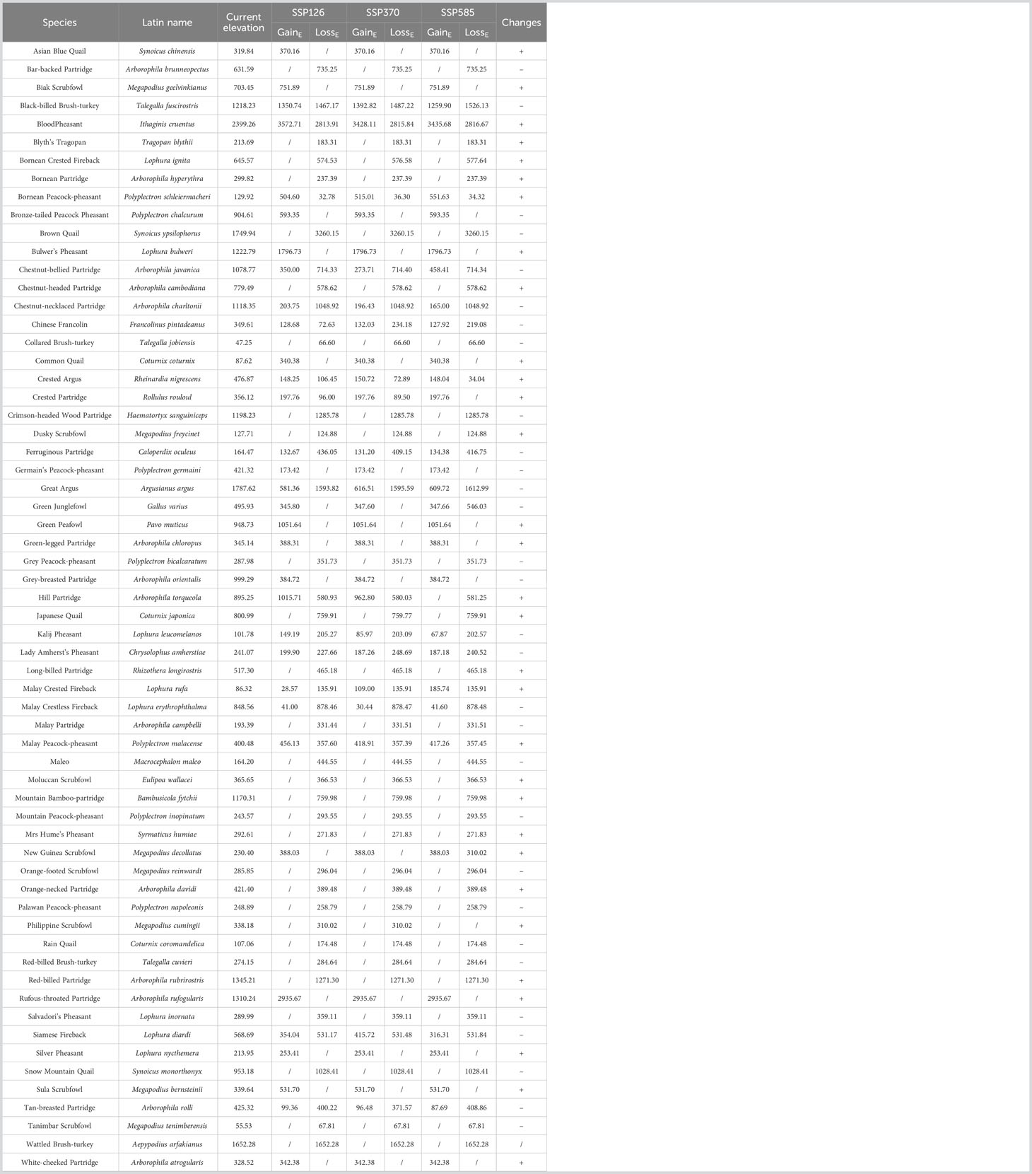
Table 3 Changes in elevation between current and future scenarios under limited dispersal scenarios.
3.4 Changes in species diversity and gap analysis
There was a significant difference in species diversity between current and future scenarios (Figures 4, 5). SDMs predicted that the area with general and medium diversity levels would obviously decrease under future scenarios, while the area with high and low diversity levels would increase.
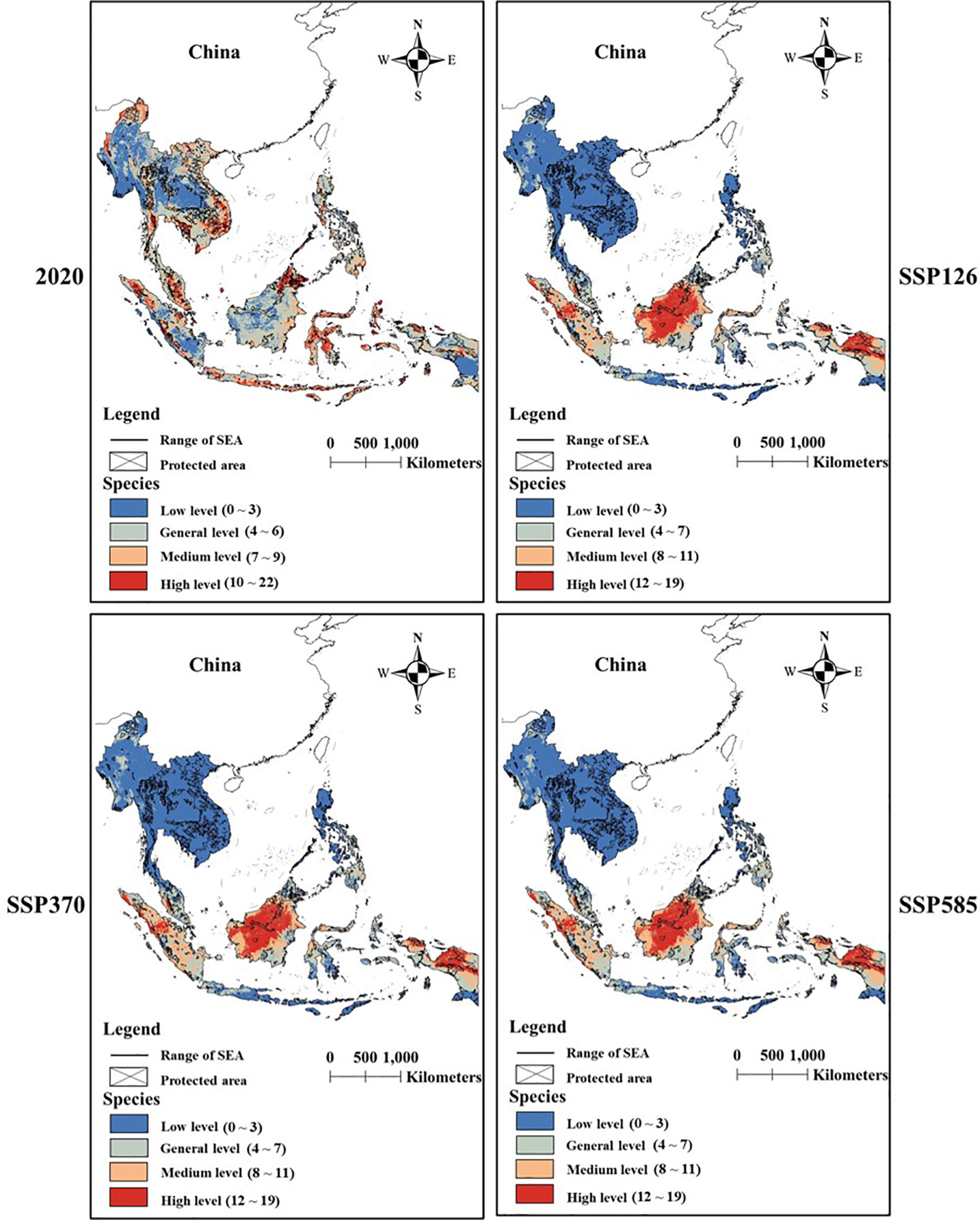
Figure 4 The difference in changes in species diversity between scenarios under perfect dispersal scenarios.
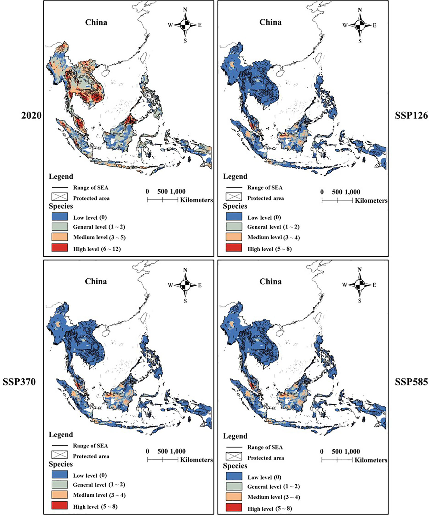
Figure 5 The difference in changes in species diversity between scenarios under limited dispersal scenarios.
At perfect dispersal scenarios, 15.53% of the suitable habitats were protected by PAs in 2020, while 16.52%, 16.48% and 16.50% of the suitable habitats would be protected by PAs under SSP126, SSP370 and SSP585. At limited dispersal scenarios, 90.89% of the suitable habitats were protected by PAs in 2020, while 21.66%, 21.15% and 20.43% of the suitable habitats would be protected by PAs under SSP126, SSP370 and SSP585.
PAs covered most areas with low diversity level under two dispersal scenarios (Figure 6). Conservation gaps for Galliformes species would mainly occur in areas with medium and high diversity levels under perfect dispersal scenarios (Figure 6A) and occur in areas with general, medium and high diversity levels under limited dispersal scenarios (Figure 6B).
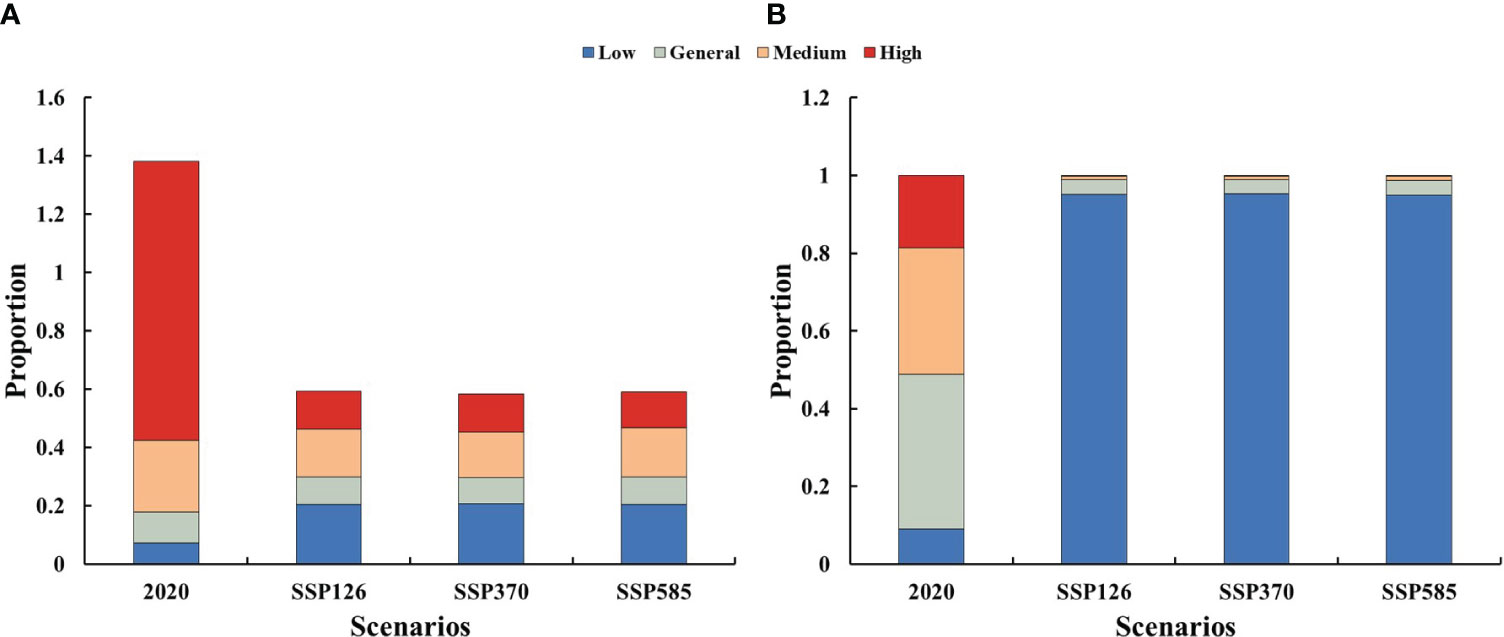
Figure 6 Protection proportion of suitable habitat with different diversity level under different scenarios. (A) Perfect dispersal scenarios; (B) Limited dispersal scenarios
4 Discussion
Our study emphasized that future climate and land-use changes would accelerate suitable habitat loss, and land use changes, Bio18, Bio13 and Bio2 were the main influencing variables. We found that precipitation of extreme quarters (Bio18 and Bio19) and temperature (Bio2) explained a large proportion of variations in potential species distribution. Temperature and precipitation are widely recognized as the factors inducing suitable habitat loss (Conrey et al., 2016; Chiatante et al., 2021; Yao et al., 2021). Long-term changes can alter physiological conditions of species, thus affecting the climatic niche (Jiang et al., 2023) and forcing species to adjust their habitat selection strategies. Moreover, temperature and precipitation also affect life cycles and food resource distribution (insects and plants) (Memmott et al., 2007; Zi et al., 2023), which makes original habitats more suitable or unsuitable for species. Our model showed that precipitation had a stronger influence on the potential distribution of Galliformes species than temperature, probably because El Nino events have once caused severe drought in Southeast Asia. Precipitation shortage and severe drought are fatal to Galliformes species, as they not only impede the growth of plants but also cause disasters such as water scarcity and forest fires (Chokkalingam et al., 2005). Water and food resources are necessary for all animals to survive, and forest fires may directly kill Galliformes.
Our results showed that land-use changes had the biggest contribution to the potential distribution of Galliformes species, and forest cover would decrease and cropland area would increase by 2080. Many researchers have confirmed that the forests of SEA are disappearing, mainly due to deforestation and infrastructure construction (Savini et al., 2021; Reddiar and Osti, 2022). For instance, in order to earn a living, indigenous people of southern Palawan exploit and supply forest products and transform forest land into cropland (Smith and Dressler, 2019). Construction of roads has provided convenient access to forests for people in Indonesia (Wilkie et al., 2000). It is worth noting that hunting is rampant in SEA and Galliformes species are the main target of hunters (Gray et al., 2018; Savini et al., 2021). Therefore, convenient access to forests may increase the hunting risks of Galliformes species. Besides, land-use changes have absolutely increased the degree of forest fragmentation (Wilson et al., 2015; Tang et al., 2020). Although the suitable habitat area of 62 Galliformes species would increase or decrease, it is still a thorny issue whether species can move from original habitats to new habitats.
It is generally believed that future climate change will force species to move to higher elevations (LaSorte and Jetz, 2010; Freeman et al., 2018; Wallingford et al., 2020). Our results also supported this opinion, and showed that 22 (perfect dispersal scenarios) or 31 (limited dispersal scenarios) of 62 species would migrate upward under future scenarios, as climate and land-use changes would reduce the habitat suitability at lower elevations. For example, we predicted that Bornean Peacock-pheasant (Polyplectron schleiermacheri), Great Argus (Rheinardia ocellata) and Green Peafowl (Pavo muticus) will shift to higher elevation. According to IUCN red list, upper elevation limit of three species was 1000m, 1500m and 2100m, respectively. This indicated that changes in elevation of these three species meet the biological characteristics. However, these species may still be faced with survival stress if forest line has no changes. A recent study has demonstrated that the elevation of future habitats for 55 Galliformes species will increase or remain stable by 2100 in SEA (Namkhan et al., 2022). On the contrary, our results showed that 42 (perfect dispersal scenarios) or 30 (limtted dispersal scenarios) of 62 species would move to lower elevations or lose a large number of distribution areas at high elevations. There may be two explanations for this phenomenon. First, these species may have better adaptability to climate and land-use changes. Second, species living in warmer areas can tolerate future temperatures (the truncated niche hypothesis) (Feeley and Silman, 2010b), so they do not need to move to higher elevations. These species would choose to live at lower elevations, probably because of the deteriorating living conditions in original habitats caused by land-use changes.
Future climate and land-use changes would expand the area with low and high diversity of Galliformes species. As we expected, suitable habitat loss would expand the area with low diversity, but the expansion of areas with high diversity was inconsistent with our expectation. We believed that the finite suitable habitat would promote species aggregation under future changes. However, Galliformes species usually have similar habits and the restricted activity areas, which may cause a fierce competition between species. Our results also showed that these high-diversity areas were mainly distributed in Borneo, Sumatra Island, Palawan island and west New Guinea, and there was an obvious gap between these areas and protected areas. In addition, our model predicted that most species tended to be distributed at lower elevations under current and future scenarios (see Table 2). For instance, Japanese Quail (Coturnix japonica), White-cheeked Partridge (Arborophila atrogularis) and Orange-necked Partridge (Arborophila davidi) also utilized artificial habitat and lowland. As a result, there may be some conflicts between Galliformes and human at lower elevations. For instance, farming and forest product trade are developing rapidly on the southeast Palawan island, and numerous rice fields and commercial coconut gardens are widely distributed in lowland coastal plains of Borneo (Smith and Dressler, 2019). These human activities will have negative impacts on the survival of Galliformes. Moreover, island habitats will be the future suitable habitats for Galliformes, and these species are thought to have a limited dispersal ability between islands. Therefore, they will eventually be at risk of extinction if these areas are not effectively protected. Our findings suggested that it was necessary to establish more PAs or adjust the range of PAs based on the combined effect of climate and land-use changes, in order to conserve 30% of the planet by 2030 (also called 30 × 30) (Convention on Biological Diversity, 2022).
We acknowledged that SDMs are a simulation of species distribution, but we still believed SDMs are useful tools for predicting current and future species distributions (Araujo and New, 2007; Kindt, 2018; Dai et al., 2021), and may provide suggestions for managers to adjust conservation policies (Michalak et al., 2018; Prahalad et al., 2019; Tian et al., 2021). A previous study has pointed out that climate change may have limited impacts on altitudinal migrant species such as blood pheasant (Ithaginis cruentus) (Fan et al., 2020; Wallingford et al., 2020; IUCN, 2023). Unfortunately, we set buffers to limit the dispersal of Galliformes, but we did not take into account species migration in this study. Although previous studies have assessed the independent effects of climate change and habitat loss on Galliformes in SEA (Savini et al., 2021; Namkhan et al., 2022), our study demonstrated that it was necessary to consider the combined impacts of both factors on Galliformes. We did not directly compare the impact of climate and land-use changes, as this was not the purpose of our study. Taken together, land-use change had a stronger impact than climate change due to its immediacy and irreversibility, but we acknowledged that the long-term effect of climate change could not be ignored. Hopefully, our results will be used as a basis for understanding the future distribution of Galliformes species in SEA and provide scientific guidance for biodiversity conservation in the future.
Data availability statement
The original contributions presented in the study are included in the article/Supplementary Material. Further inquiries can be directed to the corresponding author.
Ethics statement
The studies involving humans were approved by the Institutional Review Board of the National Center for Health Statistics. The studies were conducted in accordance with the local legislation and institutional requirements. The participants provided their written informed consent to participate in this study.
Author contributions
ZL and JX designed the study. ZL, ST, and SL developed the methods. ZL, ZZ, and LA collected the data. ZL, ZZ, YP, and XL conducted the analyses. JL, YW, and JX reviewed and edited the paper. ZL and JX wrote the paper. All authors contributed to the article and approved the submitted version.
Funding
This research was supported by the National Natural Science Foundation of China (Grant/Award Number: No.31872240).
Acknowledgments
We are grateful to the reviewers for their insightful remarks.
Conflict of interest
The authors declare that the research was conducted in the absence of any commercial or financial relationships that could be construed as a potential conflict of interest.
Publisher’s note
All claims expressed in this article are solely those of the authors and do not necessarily represent those of their affiliated organizations, or those of the publisher, the editors and the reviewers. Any product that may be evaluated in this article, or claim that may be made by its manufacturer, is not guaranteed or endorsed by the publisher.
Supplementary material
The Supplementary Material for this article can be found online at: https://www.frontiersin.org/articles/10.3389/fevo.2023.1216769/full#supplementary-material
References
Araujo M. B., New M. (2007). Ensemble forecasting of species distributions. Trends. Ecol. Evol. 22, 42–47. doi: 10.1016/j.tree.2006.09.010
Bagaria P., Thapa A., Sharma L. K., Joshi B. D., Singh H., Sharma C. M., et al. (2021). Distribution modelling and climate change risk assessment strategy for rare Himalayan Galliformes species using archetypal data abundant cohorts for adaptation planning. Clim. Riks. Manage. 31, 100264. doi: 10.1016/j.crm.2020.100264
Bos A. B., Sy V. D., Duchelle A. E., Atmadja S., Bruin S. D., Wunder S., et al. (2020). Integrated assessment of deforestation drivers and their alignment with subnational climate change mitigation efforts. Environ. Sci. Policy. 114, 352–365. doi: 10.1016/j.envsci.2020.08.002
Brambilla M., Gustin M., Cento M., Ilahiane L., Celada C. (2020). Habitat, climate, topography and management differently affect occurrence in declining avian species: Implications for conservation in changing environments. Sci. Total. Environ. 742, 140663. doi: 10.1016/j.scitotenv.2020.140663
Brodie J. F. (2016). Synergistic effects of climate change and agricultural land use on mammals. Front. Ecol. Environ. 14, 20–26. doi: 10.1002/16-0110.1
Bühne H. S., Tobias J. A., Durant S. M., Pettorelli N. (2021). Improving predictions of climate change–land use change interactions. Trends. Ecol. Evol. 36 (1), 29–38. doi: 10.1016/j.tree.2020.08.019
Carlen E. J., Li R., Winchell K. M. (2021). Urbanization predicts flight initiation distance in feral pigeons (Columba livia) across New York City. Anim. Behav. 178, 229–245. doi: 10.1016/j.anbehav.2021.06.021
Chiatante G., Giordano M., Rosin A. V., Sacchi O., Meriggi A. (2021). Spatial distribution of the Barbary Partridge (Alectoris barbara) in Sardinia explained by land use and climat. Eur. J. Wildlife. Res. 67 (4), 1–15. doi: 10.1007/s10344-021-01519-w
Chokkalingam U., Kurniawan I., Ruchiat Y. (2005). Fire, livelihoods, and environmental change in the Middle Mahakam peatlands, East Kalimantan. Ecol. Soc 10 (1), 26. doi: 10.1016/j.ecolecon.2004.10.014
Conrey R. Y., Skagen S. K., Adams A. A. Y., Panjabi A. O. (2016). Extremes of heat, drought and precipitation depress reproductive performance in shortgrass prairie passerines. IBIS 158 (3), 614–629. doi: 10.1111/ibi.12373
Convention on Biological Diversity (2022) Kunming-Montreal Global Biodiversity Framework. Available at: https://www.cbd.int/doc/c/e6d3/cd1d/daf663719a03902a9b116c34/cop-15-l-25-en.pdf.
Côté I. M., Darling E., Brown C. (2016). Interactions among ecosystem stressors and their importance in conservation. P. R. Soc B-Biol. Sci. 283, 20152592. doi: 10.1098/rspb.2015.2592
Dai Y. C., Peng G. C., Wen C. H., Zahoor B., Ma X. D., Hacker C. E., et al. (2021). Climate and land use changes shift the distribution and dispersal of two umbrella species in the Hindu Kush Himalayan region. Sci. Total. Environ. 777, 146207. doi: 10.1016/j.scitotenv.2021.146207
Estoque R. C., Ooba M., Avitabile V., Hijioka Y., DasGupta R., Togawa T., et al. (2019). The future of Southeast Asia’s forests. Nat. Commun. 10, 1829. doi: 10.1038/s41467-019-09646-4
Fan F., Bu H. L., McShea W. J., Shen X. L., Li V. B. B., Li S. (2020). Seasonal habitat use and activity patterns of blood pheasant Ithaginis cruentusbe in the presence of free-ranging livestock, Glob. Ecol. Conserv. 23, e01155. doi: 10.1016/j.gecco.2020.e01155
Feeley K. J., Silman M. R. (2010a). Silman Land-use and climate change effects on population size and extinction risk of Andean plants. Global. Change. Biol. 16, 3215–3222. doi: 10.1111/j.1365-2486.2010.02197.x
Feeley K. J., Silman M. R. (2010b). Biotic attrition from tropical forests correcting for truncated temperature niches. Global. Change. Biol. 16, 1830–1836. doi: 10.1111/j.1365-2486.2009.02085.x
Fick S. E. R. J. (2017). WorldClim 2: new 1km spatial resolution climate surfaces for global land areas. Int. J. Climatol. 37 (12), 4302–4315. doi: 10.1002/joc.5086
Freeman B. G., Lee-Yaw J. A., Sunday J. M., Hargreaves A. L. (2018). Expanding, shifting and shrinking: The impact of global warming on species’ elevational distributions. Global. Ecol. Biogeogr. 27, 1268–1276. doi: 10.1111/geb.12774
Gaüzère P., Barbaro L., Calatayud F., Princé K., Devictor V., Raison L., et al. (2020). Long-term effects of combined land-use and climate changes on local bird communities in mosaic agricultural landscapes. Agr. Ecosyst. Environ. 289, 106722. doi: 10.1016/j.agee.2019.106722
Geldmann J., Manica A., Burgess N. D., Coad L., Balmford A. (2019). A global-level assessment of the effectiveness of protected areas at resisting anthropogenic pressures. P. Natl. Acad. Sci. U.S.A. 116, 23209–23215. doi: 10.1073/pnas.1908221116
Gidey E., Dikinya O., Sebego R., Sebego R., Zenebe A. (2017). Cellular automata and Markov chain (CA_Markov) model-based predictions of future land use and land cover scenarios (2015–2033) in raya, northern Ethiopia. Model. Earth. Syst. Environ. 3, 1245–1262. doi: 10.1007/s40808-017-0397-6
Grainger M. J., Garson P. J., Browne S. J., McGowan P. J., Savini. T. (2018). Conservation status of phasianidae in Southeast Asia. Biol. Conserv. 220, 60–66. doi: 10.1016/j.biocon.2018.02.005
Gray T. N., Hughes A. C., Laurance W. F., Long B., Lynam A. J., O’Kelly H., et al. (2018). The wildlife snaring crisis: an insidious and pervasive threat to biodiversity in Southeast Asia. Biodivers. Conserv. 27, 1031–1037. doi: 10.1007/s10531-017-1450-5
Halmy M. W. A., Gessler P. E., Hicke J. A., Salem B. B. (2015). Land use/land cover change detection and prediction in the north-western coastal desert of Egypt using Markov-CA. Appl. Geogr. 63, 101–112. doi: 10.1016/j.apgeog.2015.06.015
Hansen M. C., Potapov P. V., Moore R., Hancher M., Turubanova S. A., Tyukavina A., et al. (2013). High-resolution global maps of 21st-century forest cover change. Science 342 (6160), 850–853. doi: 10.1126/science.1244693
Hidasi-Neto J., Joner D. C., Resende F., Monteiro L. D. M., Faleiro F. V., Loyola R. D., et al. (2019). Climate change will drive mammal species loss and biotic homogenization in the Cerrado Biodiversity Hotspot. Perspect. Ecol. Conserv. 17 (2), 57–63. doi: 10.1016/j.pecon.2019.02.001
Hu Y. B., Fan H. Z., Chen Y. H., Chang J., Zhan X. J., Wu H., et al. (2021). Spatial patterns and conservation of genetic and phylogenetic diversity of wildlife in China. Sci. Advances. 7 (4), eabd5725. doi: 10.1126/sciadv.abd5725
Hülber K., Kuttner M., Moser D., Rabitsch W., Schindler S., Wessely J., et al. (2020). Habitat availability disproportionally amplifies climate change risks for lowland compared to alpine species. Glob. Ecol. Conserv. 23, e01113. doi: 10.1016/j.gecco.2020.e01113
Jetz W., Wilcove D. S., Dobson A. P. (2007). Projected impacts of climate and land-use change on the global diversity of birds. PloS. Biol. 5, 157. doi: 10.1371/journal.pbio.0050157
Jiang Z. W., Ma L., Mi C. R., Tao S. A., Guo F., Du W. G. (2023). Distinct responses and range shifts of lizards populations across an elevational gradient under climate change. Global. Change. Biol. 29, 2669–2680. doi: 10.1111/gcb.16656
Johnsgard P. A. (1999). The pheasants of the world: biology and natural history (Washington DC: Smithsonian Institution Press).
Jones-Farrand D. T., Fearer T. M., Thogmartin W. E., Thompson F. R. III, Nelson M. D., Tirpak J. M. (2011). Comparison of statistical and theoretical habitat models for conservation planning: the benefit of ensemble prediction. Ecol. Appl. 21 (6), 2269–2282. doi: 10.1890/10-1047.1
Kark S., Iwaniuk A. N., Schalimtzek A., Banker E. (2007). Living in the city: can anyone become an “urban exploiter”? J. Biogeogr. 34, 638–651. doi: 10.1111/j.1365-2699.2006.01638.x
Keshtkar H., Voigt W. (2016). Potential impacts of climate and landscape fragmentation changes on plant distributions: coupling multi-temporal satellite imagery with GIS-based cellular automata model. Ecol. Inform. 32, 145–155. doi: 10.1016/j.ecoinf.2016.02.002
Kindt R. (2018). Ensemble species distribution modelling with transformed suitability values. Environ. Modell. Software 100, 136–145. doi: 10.1016/j.envsoft.2017.11.009
Krauss J., Bommarco R., Guardiola M., Heikkinen R. K., Helm A., Kuussaari M., et al. (2010). Habitat fragmentation causes immediate and time-delayed biodiversity loss at different trophic levels. Ecol. Lett. 13 (5), 597–605. doi: 10.1111/j.1461-0248.2010.01457.x
Kucuker M. A., Guney M., Oral H. V., Copty N. K., Onay T. T. (2015). Impact of deforestation on soil carbon stock and its spatial distribution in the Western Black Sea Region of Turkey. J. Environ. Manage. 147, 227–235. doi: 10.1016/j.jenvman.2014.08.017
Kyprioti A., Almpanidou V., Chatzimentor A., Katsanevakis S., Mazaris A. D. (2021). Is the current Mediterranean network of marine protected areas resilient to climate change? Sci. Total. Environ. 792, 148397. doi: 10.1016/j.scitotenv.2021.148397
LaSorte F. A., Jetz W. (2010). Projected range contractions of montane biodiversity under global warming. P. R. Soc B-Biol. Sci. 277, 3401–3410. doi: 10.1098/rspb.2010.0612
Lehikoinen A., Virkkala R. (2016). North by north-west: climate change and directions of density shifts in birds. Global. Change. Biol. 22 (3), 1121–1129. doi: 10.1111/gcb.13150
Lobo J. M., Tognelli M. F. (2011). Exploring the effects of quantity and location of pseudo-absences and sampling biases on the performance of distribution models with limited point occurrence data. J. Nat. Conserv. 19 (1), 1–7. doi: 10.1016/j.jnc.2010.03.002
Manes S., Costello M. J., Beckett H., Debnath A., Devenish-Nelson E., Grey K. A., et al. (2021). Endemism increases species’ climate change risk in areas of global biodiversity importance. Biol. Conserv. 257, 109070. doi: 10.1016/j.biocon.2021.109070
Mansour S., Alahmadi M., Atkinson P. M., Dewan A. (2022). Forecasting of built-up land expansion in a desert urban environment. Remote. Sens-Basel. 14 (9), 2037. doi: 10.3390/rs14092037
Memmott J., Craze P. G., Waser N. M., Price M. V. (2007). Global warming and the disruption of plant–pollinator interactions. Ecol. Lett. 10 (8), 710–717. doi: 10.1111/j.1461-0248.2007.01061.x
Meyer C., Weigelt P., Kreft H. (2016). Multidimensional biases, gaps and uncertainties in global plant occurrence information. Ecol. Lett. 19, 992–1006. doi: 10.1111/ele.12624
Michalak J. L., Lawler J. J., Roberts D. R., Carroll C. (2018). Distribution and protection of climatic refugia in North America. Conserv. Biol. 32, 1414–1425. doi: 10.1111/cobi.13130
Møller A. P., Diaz M., Flensted-Jensen E., Grim T., Ibáñez-Álamo J. D., Jokimäki J., et al. (2012). High urban population density of birds reflects their timing of urbanization. Oecologia 170, 867–875. doi: 10.1007/s00442-012-2355-3
Naimi B., Araújo M. B. (2016). Sdm: a reproducible and extensible R platform for species distribution modelling. Ecography 39, 368–375. doi: 10.1111/ecog.01881
Namkhan M., Sukumal N., Savini T. (2022). Impact of climate change on Southeast Asian natural habitats, with focus on protected areas. Glob. Ecol. Conserv. 39, e02293. doi: 10.1016/j.gecco.2022.e02293
Northrup J. M., Rivers J. W., Yang Z., Betts M. G. (2019). Synergistic effects of climate and land-use change influence broad-scale avian population declines. Global. Change. Biol. 25, 1561–1575. doi: 10.1111/gcb.14571
Pearce-Higgins J. W., Beale C. M., Oliver T. H., August T. A., Carroll M., Massimino D., et al. (2017). A national-scale assessment of climate change impacts on species: assessing the balance of risks and opportunities for multiple taxa. Biol. Conserv. 213, 124–134. doi: 10.1016/j.biocon.2017.06.035
Phillips S. J., Anderson R. P., Schapire R. E. (2006). Maximum entropy modeling of species geographic distributions. Ecol. Model. 190, 231–259. doi: 10.1016/j.ecolmodel.2005.03.026
Potapov P., Hansen M. C., Laestadius L., Turubanova S., Yaroshenko A., Thies C., et al. (2017). The last frontiers of wilderness: Tracking loss of intact forest landscapes from 2000 to 2013. Sci. Adv. 3 (1), e1600821. doi: 10.1126/sciadv.1600821
Powers R. P., Jetz W. (2019). Global habitat loss and extinction risk of terrestrial vertebrates under future land-use-change scenarios. Nat. Clim. Change. 9 (4), 1. doi: 10.1038/s41558-019-0406-z
Prahalad V., Whitehead J., Latinovic A., Kirkpatrick J. B. (2019). The creation and conservation effectiveness of state-wide wetlands and waterways and coastal refugia planning overlays for Tasmania, Australia. Land. Use. Policy. 81, 502–512. doi: 10.1016/j.landusepol.2018.11.009
Prasad A. M., Iverson L. R., Liaw A. (2006). Newer classification and regression tree techniques: bagging and random forests for ecological prediction. Ecosystems 9, 181–199. doi: 10.1007/s10021-005-0054-1
Reddiar I. B., Osti M. (2022). Quantifying transportation infrastructure pressure on Southeast Asian World Heritage forests. Biol. Conserv. 270, 109564. doi: 10.1016/j.biocon.2022.109564
Salvadeo C., Morzaria-Luna H. N., Reyes-Bonilla H., Ivanova-Bonchera A., Ramírez D. P., Juárez-León E. (2021). Fisher’s perceptions inform adaptation measures to reduce vulnerability to climate change in a Mexican natural protected area. Mar. Policy. 134, 104793. doi: 10.1016/j.marpol.2021.104793
Savini T., Namkhan M., Sukumal N. (2021). Conservation status of Southeast Asian natural habitat estimated using Galliformes spatio-temporal range decline. Glob. Ecol. Conserv. 29, e01723. doi: 10.1016/j.gecco.2021.e01723
Sekercioglu C. H., Schneider S. H., Fay J. P., Loarie S. R. (2007). Climate change, elevational range shifts, and bird extinctions. Cons. Biol. 22 (1), 140–150. doi: 10.1111/j.1523-1739.2007.00852.x
Selwood K. E., Zimmer H. C. (2020). Refuges for biodiversity conservation: A review of the evidence. Biol. Conserv. 245, 108502. doi: 10.1016/j.biocon.2020.108502
Shahabuddin G., Goswami R., Krishnadas M., Menon T. (2021). Decline in forest bird species and guilds due to land use change in the Western Himalaya. Glob. Ecol. Conserv. 25, e01447. doi: 10.1016/j.gecco.2020.e01447
Shen G. Z., Pimm S. L., Feng C. Y., Ren G. F., Liu Y. P., Xu W. T., et al. (2015). Climate change challenges the current conservation strategy for the giant panda. Biol. Conserv. 190, 43–50. doi: 10.1016/j.biocon.2015.05.004
Sill S. R., Dawson T. P. (2021). Climate change impacts on the ecological dynamics of two coral reef species, the humphead wrasse (Cheilinus undulatus) and crown-of-thorns starfish (Ancanthaster planci). Ecol. Inform. 65, 101399. doi: 10.1016/j.ecoinf.2021.101399
Smith W., Dressler W. (2019). Governing vulnerability: The biopolitics of conservation and climate in upland Southeast Asia. Polit. Geogr. 72, 76–86. doi: 10.1016/j.polgeo.2019.04.004
Sodhi N. S., Posa M. R. C., Lee T. M., Bickford D., Koh L. P., Brook B. W., et al. (2010). The state and conservation of Southeast Asian biodiversity. Biodivers. Conserv. 19, 317–328. doi: 10.1007/s10531-009-9607-5
Stropp J., Ladle R. J., M. Malhado A. C., Hortal J., Gaffuri J., H. Temperley W., et al. (2016). Mapping ignorance: 300 years of collecting flowering plants in Africa. Global. Ecol. Biogeogr. 25, 1085–1096. doi: 10.1111/geb.12468
Symes W. S., Edwards D. P., Miettinen J., Rheindt F. E., Carrasco R. (2018). Combined impacts of deforestation and wildlife trade on tropical biodiversity are severely underestimated. Nat. Commun. 9, 4052. doi: 10.1038/s41467-018-06579-2
Tang F., Fu M., Wang L., Zhang P. T. (2020). Land-use change in Changli County, China: Predicting its spatio-temporal evolution in habitat quality. Ecol. Indic. 117, 106719. doi: 10.1016/j.ecolind.2020.106719
Tian S., Lu S., Hua J. Q., Chang J., Li J. Q., Zhang Z. W., et al. (2021). Integrating habitat suitability modelling and assessment of the conservation gaps of nature reserves for the threatened Reeves’s Pheasant. Bird. Conserv. Int. 32 (3), 384–397. doi: 10.1017/S095927092100023X
Titeux N., Henle K., Mihoub J. B., Regos A., Geijzendorffer I. R., Cramer W., et al. (2016). Biodiversity scenarios neglect future land-use changes. Global. Change. Biol. 22 (7), 2505–2515. doi: 10.1111/gcb.13272
UNEP-WCMC (2022) Protected areas map of the world, June 2022. Available at: www.protectedplanet.net.
Urban M. C. (2015). Accelerating extinction risk from climate change. Science 348 (6234), 571–573. doi: 10.1126/science.aaa4984
Wallingford P. D., Morelli T. L., Allen J. M., Beaury E. M., Blumenthal D. M., Bradley B. A., et al. (2020). Adjusting the lens of invasion biology to focus on the impacts of climate-driven range shifts. Nat. Clim. Change 10 (5), 398–405. doi: 10.1038/s41558-020-0768-2
Wilkie D., Shaw E., Rotberg F., Morelli G., Auzel P. (2000). Roads, development, and conservation in the Congo Basin. Conserv. Biol. 14, 1614–1622. doi: 10.1111/j.1523-1739.2000.99102.x
Wilson M. C., Chen X. Y., Corlett R. T., Didham R. K., Ding P., Holt R. D., et al. (2015). Habitat fragmentation and biodiversity conservation: Key findings and future challenges. Landscape. Ecol. 31 (2), 219–227. doi: 10.1007/s10980-015-0312-3
Yao H. Y., Wang P. C., Davison G., Wang Y., McGowan P. J. K., Wang N., et al. (2021). How do Snow Partridge (Lerwa lerwa) and Tibetan Snowcock (Tetraogallus tibetanus) coexist in sympatry under high-elevation conditions on the Qinghai–Tibetan Plateau? Ecol. Evol. 11, 18331–18341. doi: 10.1002/ece3.8424
Zheng G. M. (2021). A Checklist on the Classification and Distribution of the Birds of the World. 2nd ed. (Beijing: China Science Publishing & Media Ltd (CSPM), 26–33.
Keywords: climate change, land use, Galliformes, protected area, Southeast Asia
Citation: Liu Z, Tian S, Lu S, Zhu Z, Peng Y, Li X, An L, Li J, Xu J and Wang Y (2023) Climate and land-use changes threaten the effectiveness of protected areas for protecting Galliformes in Southeast Asia. Front. Ecol. Evol. 11:1216769. doi: 10.3389/fevo.2023.1216769
Received: 04 May 2023; Accepted: 15 September 2023;
Published: 03 October 2023.
Edited by:
Wei Wang, Chinese Research Academy of Environmental Sciences, ChinaReviewed by:
Ji-Zhong Wan, Qinghai University, ChinaMingxia Zhang, Chinese Academy of Sciences (CAS), China
Copyright © 2023 Liu, Tian, Lu, Zhu, Peng, Li, An, Li, Xu and Wang. This is an open-access article distributed under the terms of the Creative Commons Attribution License (CC BY). The use, distribution or reproduction in other forums is permitted, provided the original author(s) and the copyright owner(s) are credited and that the original publication in this journal is cited, in accordance with accepted academic practice. No use, distribution or reproduction is permitted which does not comply with these terms.
*Correspondence: Jiliang Xu, eHVqaWxpYW5nQGJqZnUuZWR1LmNu
 Zhengxiao Liu
 Shan Tian
 Shuai Lu1
 Jianqiang Li