Deciphering the spatiotemporal trade-offs and synergies between ecosystem services and their socio-ecological drivers in the plain river network area

Understanding changes in ecosystem services (ESs) and quantitatively identifying the drivers that influence these changes are essential for achieving sustainable ecosystem development. In this study, multiple data sources and techniques, including meteorological data, land use/cover data, soil data, the InVEST model, and ArcGIS, were used to analyze the spatiotemporal variation characteristics of carbon storage, habitat quality, soil retention, water yield, and crop product supply in Xinghua City from 2000 to 2015. Additionally, we explored the causes of these changes and the interrelationships among these ESs. The results showed that: (1) During the study period, carbon storage and habitat quality declined, water yield fluctuated and increased, and soil retention had small interannual variations. The supply capacity of crop products first increased rapidly and then stabilized. (2) ESs were influenced by multiple drivers, with altitude having the strongest explanatory power for habitat quality and soil retention, and food production having the strongest explanatory power for crop product supply. (3) Relationships between different ESs were variable and changed over time. This study could enrich the understanding of spatial and temporal changes and drivers of ESs in the plain river network area, which has important implications for future land use planning and sustainable development of ESs.

1 Introduction

Ecosystem services (ESs) are a variety of direct and indirect benefits provided by natural ecosystems to human societies, including provisioning services, regulating services, cultural services, and supporting services. These services are important for human well-being, socio-economic development, and the sustainability of ecosystems (Millennium Ecosystem Assessment (MA), 2005; Costanza et al., 2014; IPBES, 2019). With continuous changes in the natural environment and rapid socio-economic development, factors such as climate, land use change, and other human activities constantly influence the spatiotemporal distribution of ESs. Also, as humans are selective about different ESs, they usually change the supply capacity of a certain ES artificially, so that the dynamic changes among various ESs are manifested as trade-off relationships or synergistic relationships of mutual promotion (Li et al., 2013; Zhong et al., 2020).

Relevant studies have found that different natural-socio-economic drivers affect ESs in different ways (Zhang et al., 2018; Dade et al., 2019; Dun et al., 2019), e.g. climate change directly induces changes in ESs such as food production, water yield services, net primary productivity, etc. and indirectly affects the capacity to provide services such as soil retention and carbon storage (Grimm et al., 2016; Uniyal et al., 2023). Changes in land use/cover directly reflect the ecosystem composition, patterns, and change processes in an area. This directly influences the spatiotemporal distribution patterns and evolutionary patterns of ESs (Zheng et al., 2019). In-depth research and understanding of the drivers of ESs are important for identifying spatial and temporal changes in ESs, predicting future trends of changes, and developing adaptive and sustainable management strategies. However, most studies have used traditional correlation or regression analyses, which focus mainly on the influence of values on drivers and ignore the spatial heterogeneity of the drivers themselves (Jia et al., 2022). Geographical detector is a new tool for geographic research that can effectively analyse the spatial heterogeneity of geographic phenomena (Han et al., 2015; Wang and Xu, 2017), and this method has been gradually applied to identify the spatially stratified characteristics of land use and landscape patterns, and it can effectively detect spatial differences and major causes in geographic phenomena (Ren and Cao, 2022; Xu et al., 2022).

Relationships between ESs involve trade-offs and synergies (Turner et al., 2014). Trade-off means that increasing or improving one ES leads to a reduction or degradation of other ESs, e.g., research has found that using more land for agricultural production increases food production but may lead to a reduction in ecosystem biodiversity (Zhao et al., 2020). Synergistic effect means that increasing or improving one ES will promote the increase or improvement of other ESs, e.g. synergistic relationship exists between pasture supply and wind and sand control, water conservation, and soil preservation in key ecological function areas in northern China (Zhu et al., 2020). Many scholars have conducted in-depth studies of the trade-offs and synergistic effects of relationships between ESs. Studying trade-offs and synergistic relationships of ESs can provide guidance for future decision-making, which can help policy makers better predict and understand the implications of favouring one ES over another (Rodríguez et al., 2006), thus avoiding potential negative impacts. It also provides a basis for decision making to achieve sustainable management of regional ecosystems, guide the future exploitation of natural resources, and improve human well-being; this is the key to transitioning from theoretical research to practical management of ESs (Fu and Yu, 2016; Zhao et al., 2020; Gao et al., 2022; Xue et al., 2023).

Xinghua is abundant in agricultural resources and is one of the most representative agricultural cities in Jiangsu Province and even in China, and the city’s total grain output has always been at the forefront in China (Cheng et al., 2011). In addition, Xinghua is rich in water resources with lakes and lagoons accounting for half of the total number of Lixia River Basin (Bai et al., 2014). Xinghua possesses ecological redline protection areas that cover one-fifth of the municipal territory. These areas have significant ecological value and require strict conservation measures. In recent years, with rapid economic development, urban land use has been expanding, which encroaches on and destroys a large amount of arable land and other ecological land. In order to pursue higher economic benefits, the trend of non-food production has become more obvious, and the area of lakes and water systems has been decreasing (Zhang, 2022). This irrational land use transition has caused great impacts on ESs, which will exacerbate the reduction of arable land resources, the pressure on water supply, and the weakening of ESs, thus threatening the sustainable development of Xinghua City. However, research on the impact of these issues on ESs in Xinghua has not yet been conducted, and how socio-economic factors will affect ESs and the relationship between ESs is not yet clear. Therefore, five key ESs, carbon storage (CS), habitat quality (HQ), soil retention (SR), water yield (WY), and crop product supply (CP), were selected for this study. The spatial and temporal changes of five ESs in Xinghua from 2000 to 2015 were analysed using Geographic Information System (ArcGIS) techniques and the InVEST model. The main drivers of change in the five ESs and their interactions had been analysed by the geographical detector. Finally, the trade-offs and synergistic relationships of the ESs were investigated using the Statistical Product and Service Solutions (SPSS) platform and correlation analysis. This study aimed to: (1) assess the spatial and temporal distribution characteristics of ESs in the study area; (2) identify the main drivers of spatiotemporal changes in ESs; (3) recognize ESs interrelationships in the study area.

2 Materials and methods

2.1 Study area

Xinghua (32°44′–33°13′ N, 119°43′–120°16′ E) is located on the northern flank of the Yangtze River Delta, between Jiang and Huai; it lies in the hinterland of the Lixia River in central Jiangsu (Peng, 2006). The terrain is low-lying and flat, with a total area of 2393.35 km², and ground elevations ranging from 1.40 to 3.20 m. The topography is high in the east and south, and low in the northwest, which is the lowest among the three main depressions of Jianhu, Xinghua, and Qintong in the Lixia River area (Ye et al., 2011). Xinghua is characterized by a subtropical humid monsoon climate, with an average annual temperature of approximately 15.5°C and average annual precipitation of 1070.76 mm. The seasonal precipitation distribution is uneven, with rainfall during the flood season (May−September) accounting for approximately 67.4% of the annual precipitation and a multi-year average annual evaporation is approximately 825.97 mm. Special geographic conditions have shaped the natural landscape of rivers and lakes in the territory, with 12,124 small, medium, and large rivers having a total length of 10,526 km and a water surface rate of 14.71% (Figure 1); it is a typical plain river network area.

FIGURE 1

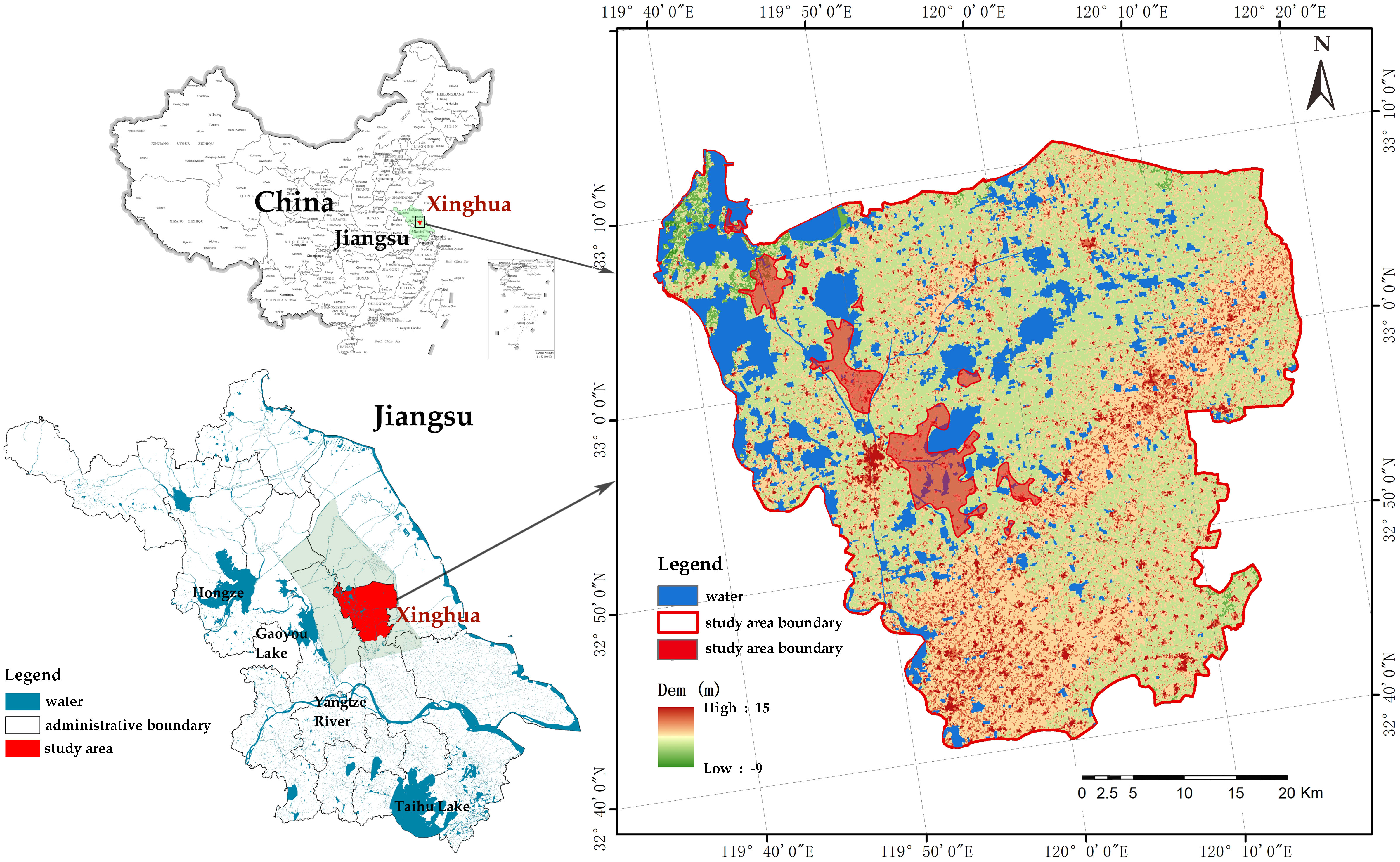
Figure 1 Location of the study area.

However, driven by economic interests, enclosures and aquaculture activities have resulted in a reduction of the water area from 26% to 18% of the lake system. At the same time, pollution from aquaculture and other production and domestic activities has posed a significant threat to the water ecosystem (Zhang, 2022). During the process of land transfer, there has been a clear trend of non-food production, with most farmers using arable land to dig ponds for aquaculture or to grow other cash crops, while only a few large grain farmers have continued to grow staple crops. These shifts in land use types have directly led to changes in the layout of arable land and permanent basic farmland, as well as ecological issues such as soil erosion and water pollution (Wang et al., 2019), negatively impacting regional ecosystem services.

2.2 Data sources and descriptions

The data required for this study mainly includes land use type, digital elevation model (DEM) data, meteorological data, soil and socio-economic data. After obtaining the relevant data, vector–grid conversion was carried out and all data were projected to the WGS84 coordinate system. For the land use type data, land resources and their utilization attributes were classified into 11 types according to China’s land use/land cover remote sensing monitoring data classification system: paddy field, dry land, woodland, grassland, canal, lake, reservoir, beach land, urban land, other construction land, and rural land. Details of the multi-source data are shown in Table 1.

TABLE 1

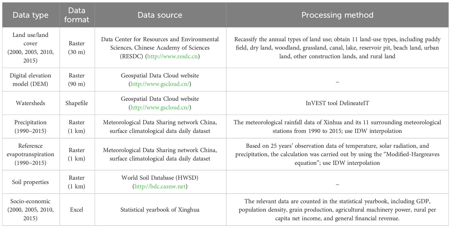
Table 1 Data sources and processing instructions.

2.3 Ecosystem services assessment

The study used the InVEST model, which has been widely used for ESs assessment and which, in combination with ArcGIS, allows the spatial representation of ES and facilitates the observation of the spatial distribution and changes in ESs (Posner et al., 2016; Hu et al., 2023).

(1) Carbon storage (CS)

The Carbon module of the InVEST model was used to estimate the carbon storage service, which mainly includes four carbon pools, including aboveground biomass, belowground biomass, soil carbon density, and carbon density of dead organic matter. The LULC maps and the stocks of the four carbon pools were entered into the model, resulting in the final output of the carbon storage raster. The calculation formula was as follows:

$\begin{array}{ll}\begin{array}{c}{C}_{toil}=C_{above}+C_{below}+C_{soil}+C_{dead}\end{array}& (1)\end{array}$

where C_toil is the total carbon storage (t/hm²), C_above is the aboveground biomass (t/hm²), C_below is the belowground biomass (t/hm²), C_soil is the soil carbon density (t/hm²), and C_dead is the carbon density of dead organic matter (t/hm²). More information about the model can be available in the Supplementary Material.

(2) Habitat quality (HQ)

Habitat quality was evaluated using the habitat quality module of the InVEST model. HQ refers to the ecosystem’s ability to provide resources for survival, reproduction, and population sustainability (Hu et al., 2023). The module calculated habitat quality by inputting LULC maps, threat rasters, the sensitivity of land cover types to each threat, and threat parameters. The calculation formula was as follows:

$\begin{array}{ll}\begin{array}{c}{Q}_{xj}=H_j\left[1-\left(\frac{D_{xj}^z}{k^z+D_{xj}^z}\right)\right]\end{array}& (2)\end{array}$

where j is the cover/use type of some land, Q_xj is the habitat quality index for raster cell x in land use type j, H_j is the habitat suitability for land use type j, D_xj is the degree of habitat degradation in raster cell x in land use type j, k is a half-saturation constant, generally taken as half of the maximum value of habitat degradation, and z is the default parameter of the model, usually takes the value of 2.5. Definitions of relevant terms and parameters are given in the Supplementary Material.

(3) Soil retention (SR)

Soil retention is represented by the difference between potential soil erosion and actual soil erosion, that is the difference between soil erosion caused by no land cover or land management measures and soil erosion under current vegetation cover management and soil and water conservation measures. The Sediment Delivery Ratio module in the InVEST model was used to analyze the soil retention capacity in the study area. The calculation formula was as follows:

$\begin{array}{ll}\begin{array}{c}\mathit{\text{USLE}}=\mathit{\text{R}}\times \mathit{\text{K}}\times \mathit{\text{LS}}\times \mathit{\text{C}}\times \mathit{\text{P}}\end{array}& (3)\end{array}$

$\begin{array}{ll}\begin{array}{c}\mathit{\text{RKLS}}=\mathit{\text{R}}\times \mathit{\text{K}}\times \mathit{\text{LS}}\end{array}& (4)\end{array}$

$\begin{array}{ll}\begin{array}{c}\mathit{\text{SD}}=\mathit{\text{RKLS}}-\mathit{\text{USLE}}\end{array}& (5)\end{array}$

where USLE is the actual soil erosion (t/hm²), RKLS is the potential erosion of soil (t/hm²). R is the rainfall erosivity, K is the soil erodibility, which was computed through the erosion-productivity impact calculator (EPIC) first proposed by Williams (Williams et al., 1984). LS is the slope length factor (topographic factor), C is the vegetation cover factor, and P is the Soil and water conservation measure factor. More information about the model can be available in the Supplementary Material.

(4) Water yield (WY)

The water yield module in the InVEST model was used to evaluate water production services. Based on the principle of water balance, this module combines climate, topography, vegetation, soil, and other factors to quantitatively evaluate the water yield of each land use in a grid (Yang et al., 2020). WY is defined as the difference between precipitation and actual evapotranspiration of each grid cell. The formula was as follows:

$\begin{array}{ll}\begin{array}{c}{Y}_x=\left(\mathbf{1}-\frac{{\mathrm{AET}}_x}{P_x}\right)\times P_x\end{array}& (6)\end{array}$

where Y_x is the annual water yield of grid cell x (mm), AET_x is the actual annual evaporation (mm) from grid x, and P_x is the average annual precipitation (mm) for raster x. More information about the model can be available in the Supplementary Material.

(5) Crop product supply (CP)

Food supply is one of the most basic supply services in ecosystem services (Liu et al., 2022). Combined with the crop production of Xinghua, four major production crops: grain, cotton, vegetables, and fruits were used to comprehensively measure the crop supply capacity of each township in Xinghua. Crop yield was calculated by using a yield model with the following formula:

$\begin{array}{ll}\begin{array}{c}\mathit{\text{PRO}}={\sum }_{\mathit{\text{i}}=\mathbf{1}}^{\mathit{\text{i}}}{A}_i\times R_i\times P_i\end{array}& (7)\end{array}$

where PRO is the yield of the crop, A_i is the area of each township in Xinghua, R_i is the area proportion of crops in each township, and P_i is the yield per unit area of crops in each township. All data came from Xinghua Statistical Yearbook from 2000 to 2015.

2.4 Impact of land use change on ecosystem services

To analyse the impact of land use change on ESs, we used the land use data downloaded from Data Center for Resources and Environmental Sciences, Chinese Academy of Sciences for the four periods of 2000/2005/2010/2015, and then imported into ArcGIS to be processed to obtain the land use distribution map of the study area for each year. Then, based on the assessment results of the five ESs above, the land use maps of each year and the spatial distribution maps of each ESs of the corresponding year were overlaid in ArcGIS to count the value of ESs on each land use type. The statistical results were divided by the total area of the study area, and the results obtained were taken as the degree of contribution of different land use types to the ESs per unit area.

2.5 Geographical detector and drivers

Geographical detector is a statistical method used to study the spatial differences of geographical phenomena and reveal the drivers behind them (Ge et al., 2021; Ji et al., 2021); it consists of four modules: risk detection, factor detection, ecological detection, and interaction detection. Geographical detector is subject to fewer prerequisite constraints and has significant advantages when dealing with mixed types of data. Factor detection and factor interaction detection modules were used in this study. The factor detector was used to detect the spatial heterogeneity of the dependent variable (ESs), and the magnitude of the q-value was used to describe the strength of spatial consistency between the drivers and ESs, as shown in Equation (8). The interaction detector detected whether the drivers X1 and X2 together enhanced or weakened the explanatory power of the ESs, or whether the effects of these drivers on ESs were independent of each other (Wang and Xu, 2017).

$\begin{array}{ll}\begin{array}{c}\mathbf{\text{q}}=\mathbf{1}-\frac{\mathbf{1}}{\mathit{\text{n}}{\mathit{\text{σ}}}^{\mathbf{2}}}{\sum }_{\text{h}=1}^{\text{L}}{\text{n}}_{\text{h}}{\sigma }_{\text{h}}^2\end{array}& (8)\end{array}$

where q denotes the explanatory power of the drivers, n denotes the sum of sample points, σ² denotes the sum regional variance, h = 1,2,3…L denotes the layer of factor X, n_h and σ_h² denote the number of sample points and variance of layer h. The q-statistic is between 0 and 1. The larger the q-statistic, the greater the explanation of ESs by the drivers.

Based on previous studies (Jopke et al., 2015; Liu et al., 2019a; Dou et al., 2020; Huang et al., 2022) combined with the target study area and data availability, 11 drivers were selected as independent variable drivers: natural drivers, including elevation, slope, temperature, potential evapotranspiration, and precipitation; and socio-economic drivers, including gross domestic product (GDP), population density, grain production, agricultural machinery power, rural per capita net income, and general financial revenue.

2.6 Quantitative measure of trade-offs and synergies between ESs

This study used the Pearson correlation coefficient method in SPSS 25.0 software to quantify the relationships between ESs. This method identifies ES trade-offs and synergistic relationships by simply quantifying statistical associations between pairs of ESs (Dade et al., 2019); it has been used previously by a large number of scholars (Sun and Li, 2017; Liu et al., 2019b; Fan et al., 2022). A positive correlation coefficient, subject to a 1% significance test, indicates a synergistic relationship between the two ESs; a negative correlation coefficient constitutes a trade-off relationship. The closer the correlation coefficient is to zero, the weaker the trade-off or synergistic relationship is between the ESs (Wu et al., 2021; Chen et al., 2022). The calculation formula was as follows:

$\begin{array}{ll}\begin{array}{c}{R}_{xy}=\frac{{\sum }_{\mathit{\text{n}}=\mathbf{1}}^{\mathit{\text{n}}}(X_{ij}-\overline{\mathit{\text{X}}})({\mathit{\text{Y}}}_{ij}-\overline{\mathit{\text{Y}}})}{\sqrt{{\sum }_{\mathit{\text{n}}=\mathbf{1}}^{\mathit{\text{n}}}{(X_{ij}-\overline{\mathit{\text{X}}})}^{\mathbf{2}}}\sqrt{{\sum }_{\mathit{\text{n}}=\mathbf{1}}^{\mathit{\text{n}}}{(Y_{ij}-\overline{\mathit{\text{Y}}})}^{\mathbf{2}}}}\end{array}& (9)\end{array}$

where R_xy is the partial correlation coefficient between services x and y, X_i and Y_i are the values of the x and y services, respectively, i and j are the row and column numbers of raster data elements, respectively, $\overline{\mathit{\text{X}}}$ and $\overline{\mathit{\text{Y}}}$ are the average values of the corresponding services, and n is the time series of the raster data.

3 Results

3.1 Spatiotemporal characteristics of ESs

3.1.1 Temporal dynamic of ESs

The average CS, HQ, SR, WY, and CP of the study area over the 15 years from 2000 to 2015 were 2363.16 Mg/c, 698.76 (dimensionless), 1.57 × 10⁵ t/pixel, 8.57 × 10⁵ mm, and 1.00 × 10⁸ t, respectively. The ESs capacity showed different degrees of variability across the four periods. Overall, during the study period (Figure 2), CS and HQ decreased by 1.60% and 0.87%, respectively; SR was lowest in 2005 and varied less in the remaining years; WY increased by 235.18%, and the four-year trend of WY was in line with the trend of mean annual precipitation. CP increased considerably from 2000 to 2010 and varied less from 2010 to 2015, increasing by 33.25% throughout the study period.

FIGURE 2

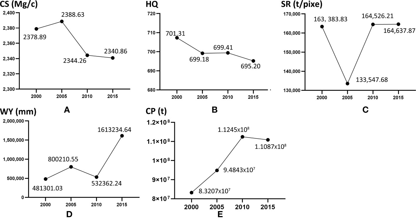
Figure 2 Temporal variation of the five ESs from 2000 to 2015. (A) Carbon storage (CS) variation over time. (B) Habitat quality (HQ) variation over time. (C) Soil retention (SR) variation over time. (D) Water yield (WY) variation over time. (E) Crop production supply (CP) variation over time.

3.1.2 Spatial dynamic of ESs

Figure 3 shows the spatial distributions of CS, HQ, SR, WY, and CP in Xinghua, where it can be seen that there are differences in the spatial distribution of each service. The high-value areas of CS are widely distributed, mainly in the areas of arable land (paddy fields and dry land) and woodland, but with the occupation of arable land by urban land, rural land, and water reservoirs, there is a decreasing trend in carbon stock; the low-value area of CS is mainly concentrated in the northwest. The high-value areas of HQ are scattered in the lake area in the northwest corner, but there is a decreasing trend accompanying the year-on-year decrease in lake area; the low-value areas of HQ are widely distributed. The spatial pattern of SR is similar across the four periods, with medium-value areas widely distributed and low-value areas mainly distributed in lakes, along water systems, and in urban land; a decreasing trend accompanies the expansion of urban and rural land. The high-value areas of WY are concentrated in the urban center and southeast, and low-value areas are widely distributed. The high-value area of CP is concentrated in the southeast, far from the urban center, and the range of the high-value area gradually expands with time; low-value areas are mainly concentrated in urban and rural land.

FIGURE 3

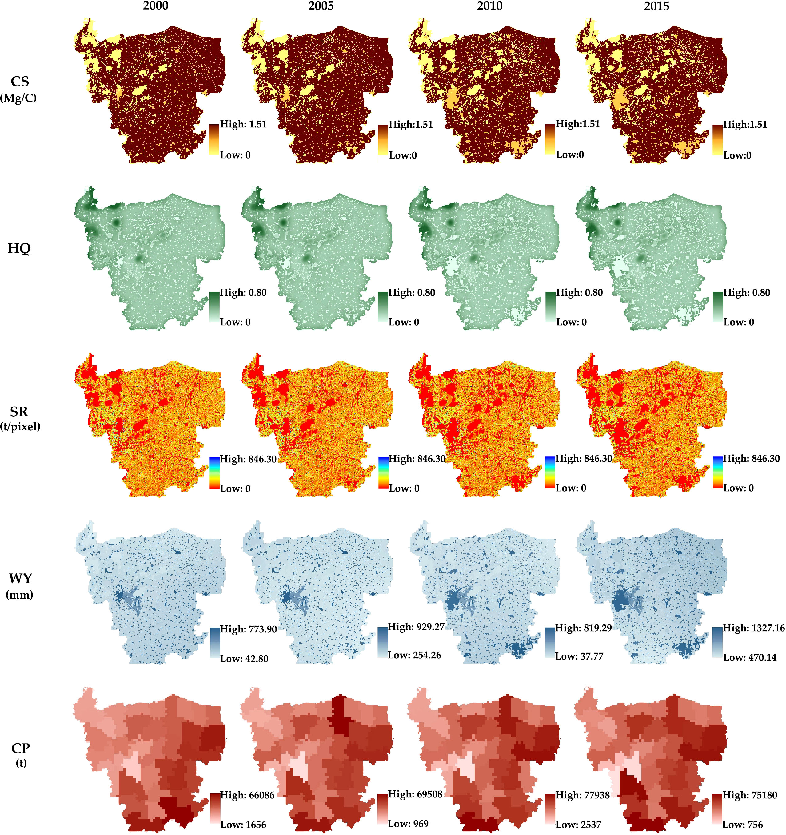
Figure 3 Spatial distributions of ESs and changes in Xinghua from 2000 to 2015 (CS, carbon storage; HQ, habitat quality; SR, soil retention; WY, water yield; CP, crop product supply).

3.2 Spatiotemporal characteristics of land use and the contribution of different land use types to ESs

Figure 4 shows the spatial distribution of land use in Xinghua from 2000 to 2015. Paddy fields were distributed most widely, and urban land was mainly concentrated in the northwestern and southeastern corners of Xinghua, mostly near river systems. From 2000 to 2015, the land use type in Xinghua was dominated by paddy fields, accounting for 71.3%−79.21% of the total area. In general, the areas of different land use types changed by different degrees. During the study period, the areas of arable land (paddy fields and dry land), grassland, and rivers (canals, lakes, and beach land) showed different degrees of decrease, among which, paddy fields decreased by 9.89%, dry land decreased by 9.64%, grassland disappeared, canals decreased by 3.65%, lakes decreased by 51.01%, and beach land decreased by 33.01%. Urban land, woodland, reservoirs, and rural land increased significantly, among which urban land showed the largest increase (365.91%), with large areas concentrated in the central, western, and southeastern corners of the city; woodland increased by 271.21%, reservoirs increased by 89.77%, and rural land increased by 13.80% (Table 2). The rapid expansion of urban land was mainly based on arable land (paddy fields and dryland).

FIGURE 4

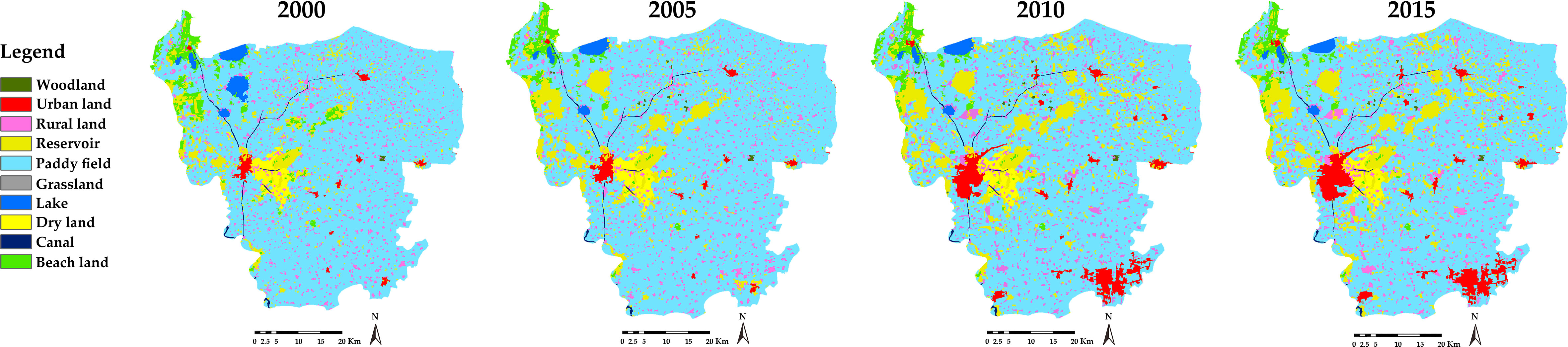
Figure 4 Spatial distributions of land use in Xinghua from 2000 to 2015.

TABLE 2

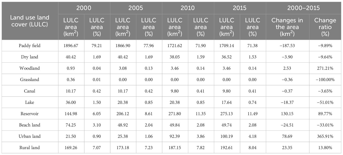
Table 2 Areas and proportions of land cover in Xinghua from 2000 to 2015.

Figure 5 shows the contribution of different land use types to the five ESs per unit area in Xinghua from 2000 to 2015. The results show that among different land use types, woodland, grassland, and arable land (paddy fields and dryland) have the strongest CS capacity; various river systems contribute the most to HQ; and the SR capacity is similar in different land types, with woodland having the highest contribution value, and woodland and paddy fields having high CP capacity.

FIGURE 5

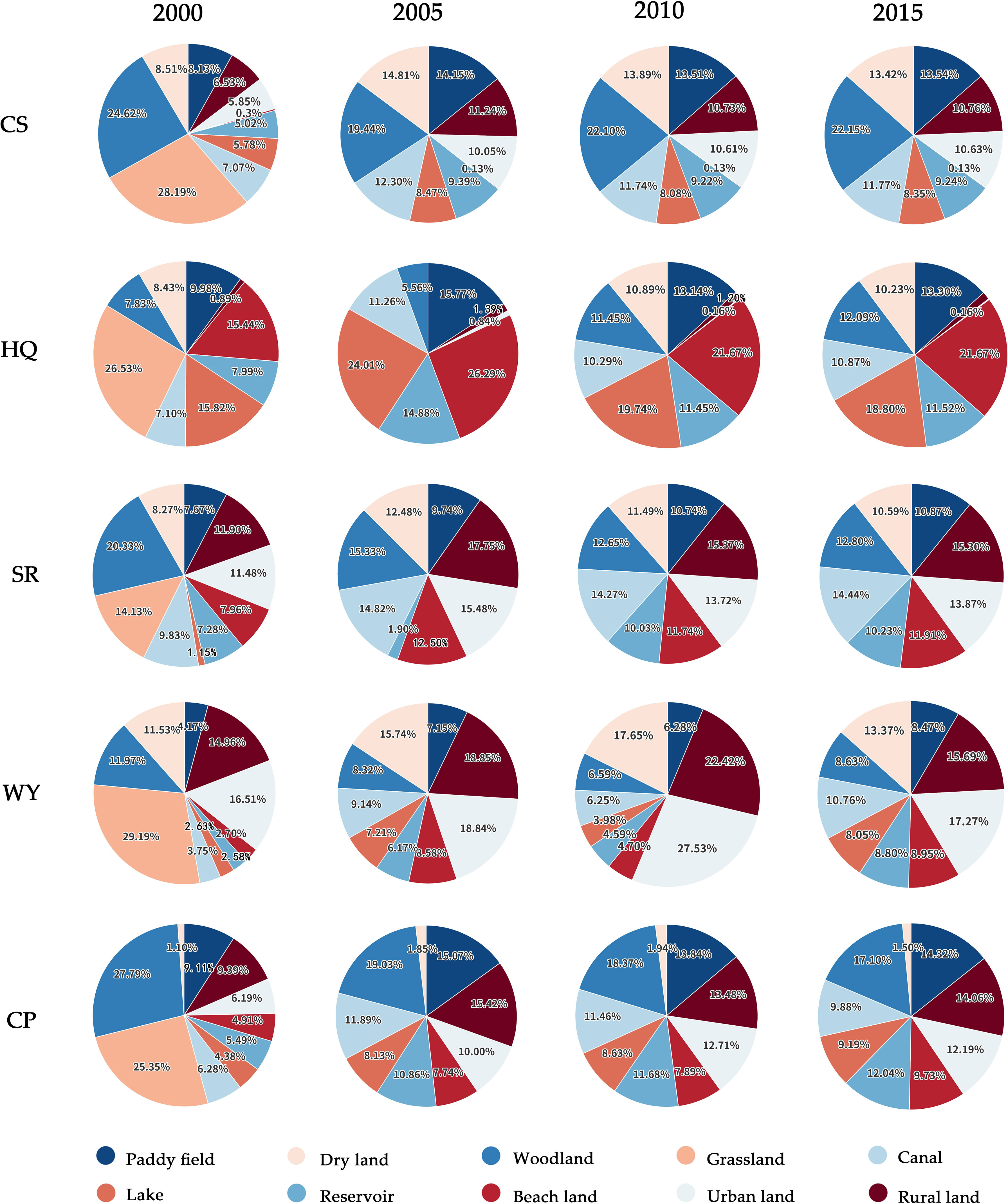
Figure 5 Contribution of different land cover types to multiple ESs per unit area from 2000 to 2015 (CS, carbon storage; HQ, habitat quality; SR, soil retention; WY, water yield; CP, crop product supply).

3.3 Drivers identification

3.3.1 Factor detector

The explanatory power of different drivers for ES in Xinghua City from 2000 to 2015 was explored using the geographical detector (Figure 6). We can see that elevation has the strongest explanatory power for HQ, with a q-value of more than 0.25, followed by general financial revenue and rural per capita net income. The strongest explanatory power for CP is grain production (0.88–0.95), followed by GDP and agricultural machinery power. Overall, socio-economic drivers have a significant impact on the variation of CP. The most dominant driver of SR is elevation (0.24–0.28), while the remaining drivers have low explanatory power. The low explanatory power of all drivers on CS and WY implies that these two ESs may be influenced by several drivers.

FIGURE 6

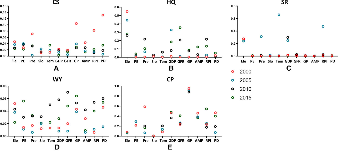
Figure 6 Factor detection results of drivers of ESs changes in Xinghua City from 2000 to 2015. (A) Carbon storage (CS) change drivers detection results. (B) Habitat quality (HQ) drivers factor detection results. (C) Soil retention (SR) drivers factor detection results. (D) Water yield (WY) drivers detection results. (E) Crop production supply (CP) drivers detection results. (Ele, elevation; PE, potential evapotranspiration; Pre, precipitation; Slo, slope; Tem, temperature; GDP, gross domestic product; GFR, general financial revenue; GP, grain production; AMP, agricultural machinery power; RPI, rural per capita net income; PD, population density).

The explanatory power of each driver for ES shows a fluctuating trend over time. The explanatory power of elevation declined for HQ, while the explanatory power of general financial revenue increased. For CP, the explanatory power of grain production and agricultural machinery power declined as a whole, while the explanatory power of general financial revenue and rural per capita net income increased as a whole. This indicates that with an increase in agricultural technology level, the effort of the government to support the agricultural impact on product supply capacity space differentiation gradually strengthens.

3.3.2 Interaction detector

The results of the interaction detection revealed that the combined effect of two drivers had stronger explanatory power than a single driver (Figure 7), with the ESs with significantly stronger explanatory power after driver interaction included HQ, SR, and CP. For HQ, elevation (X1) had the strongest interaction with the other drivers, with q-values ranging from 0.30 to 0.83; again demonstrating the importance of elevation on the explanatory power of HQ. For SR, elevation (X1) and precipitation (X3) had the most significant interaction results, with an explanatory power of 0.55–0.87. For CP, all drivers showed strong interactions, with grain production (X8) interacting significantly with the other drivers, indicating that grain production (X8) occupies a central position in CP.

FIGURE 7

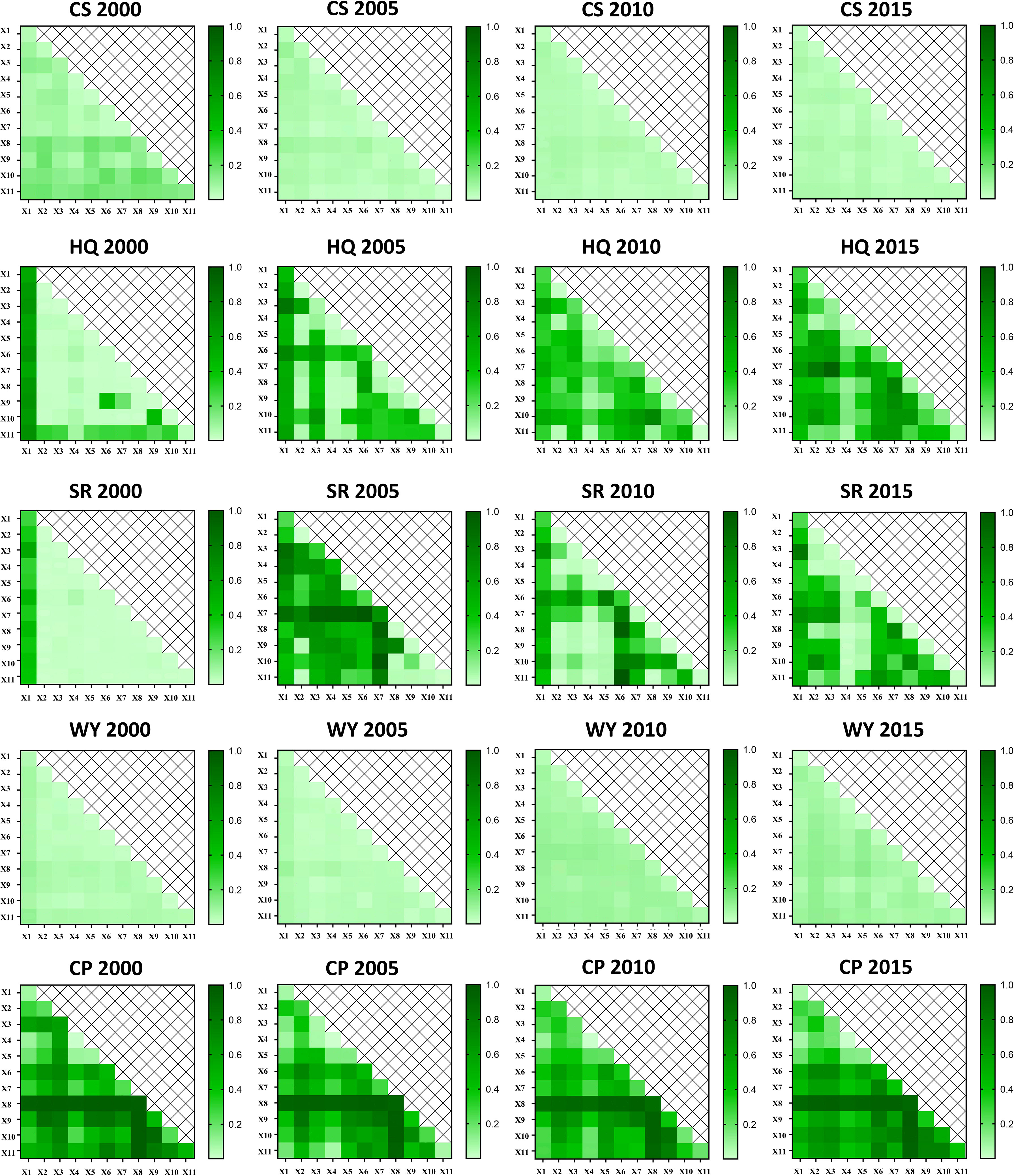
Figure 7 Interaction detection results of driver factors of ESs change in Xinghua (X1, elevation; X2, potential evapotranspiration; x3, precipitation; X4, slope; X5, temperature; X6, GDP; X7, general financial revenue; X8, grain production; X9, agricultural machinery power; X10, rural per capita net income; X11, population density; CS, carbon storage; HQ, habitat quality; SR, soil retention; WY, water yield; CP, crop product supply).

3.4 Trade-off and synergy between ESs

The correlation analysis of the five ESs in Xinghua City from 2000–2015 (Table 3) shows that there are both trade-offs and synergistic relationships among them. Carbon storage–habitat quality (CS-HQ), carbon storage–crop product supply (CS-CP), and soil retention–water yield (SR-WY) have synergistic relationships. Trade-off relationships existed for carbon storage–water yield (CS-WY), habitat quality–soil retention (HQ-SR), habitat quality–water yield (HQ-WY), and habitat quality–crop product supply (HQ-CP). Overall, trade-offs dominated the relationships among ESs in Xinghua City during the study period.

TABLE 3

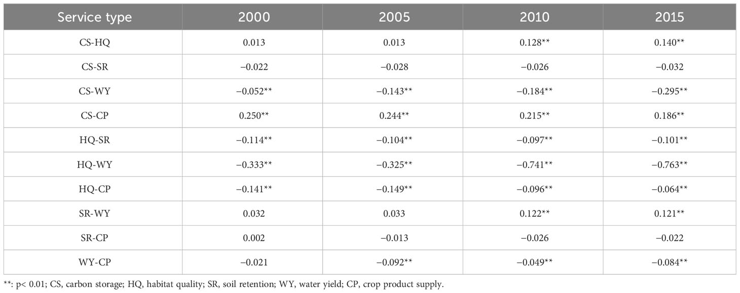
Table 3 Correlation of ESs in the study area.

4 Discussion

This study found that the ESs in the study area changed continuously in time and space during the period 2000–2015. The spatial and temporal heterogeneity of ESs was closely related to land use changes and driven by various socio-ecological drivers. Land use in Xinghua City changed significantly during the study period, with a dramatic expansion of urban construction land and an increase in forested land area. The area of arable land, grassland, and natural waters decreased. This was mainly caused by urban expansion and the conversion of arable land, grassland, wetlands, and natural waters into roads or other construction facilities (Forman, 2014). The results of the study showed that woodland, arable land (paddy fields and dryland), and grassland contributed the most to ecosystem services, and they dominated the local ESs. Especially in terms of regulating and supporting services, the ESs of these three land-use types were generally higher than those of urban land and rural land. This spatial distribution pattern was consistent with the findings in Zengcheng (Sun and Li, 2017), the western region of Suzhou (Zhao and Li, 2022), and the Taihu basin (Bai et al., 2020), which could be attributed to low anthropogenic disturbance and high natural vegetation cover. However, the degradation of CS and HQ with the expansion of the city reflected the negative impact of rapid urbanisation on ESs.

In addition, it was found that the dominant drivers were different for different ESs and that the effect of the interaction of the two drivers on ESs was enhanced, which is consistent with the results of existing related studies (Meacham et al., 2016; Lu et al., 2021; Shen et al., 2021). Among the natural drivers, elevation had the strongest explanatory power for HQ and SR. HQ and SR were relatively low in high-elevation areas, which was because of the low-lying and flat topography of Xinghua City, where urban and rural lands were mainly distributed in high-elevation areas. These areas have undergone extensive development and construction, and the natural ecosystem system has been seriously damaged. Among the socio-economic drivers, food production had the strongest explanatory power for CP, followed by GDP, agricultural machinery, and general financial income. This shows that as the level of socio-economic development increases over time, the core influence on ESs gradually shifts from natural factors to socio-economic drivers.

Understanding the trade-offs and synergies among ESs is important for guiding policy formulation, optimising resource use, and protecting ecosystems (Howe et al., 2014; Cord et al., 2017). After examining the trade-offs and synergies between ESs in the study area, we found that the relationships between ESs showed heterogeneity during the study period. Among them, the most significant changes were CS-CP, CS-WY, and HQ-WY. The degree of synergy between CS-CP weakened over time, which could be attributed to the fact that the rapid development of urbanisation occupied a large amount of arable land, resulting in a decrease in organic carbon fixed by crops. On the other hand, the increase in food production per unit area and the improvement in agricultural mechanisation were conducive to the increase in CP (Long-hui et al., 2020; Zhang et al., 2023). The combined effect of these two factors weakened the synergy between CS and CP. Secondly, the degree of trade-off between CS-WY was increased, mainly due to the expansion of urban land use and the increase in annual rainfall. Combined with Figures 2 and 4, it is suggested that the high value of WY was mainly located in the urban land, which was due to the expansion of urban land that not only increased the demand for water resources but also led to a decrease in evapotranspiration and an increase in water production capacity (Ji et al., 2022; Wu et al., 2022). The expansion of urban land was mainly through the occupation of arable land, and the reduction of arable land led to a decrease in organic carbon, so the degree of trade-off between CS-WY increased. The degree of trade-off between HQ-WY also increased, as the expansion of urban land and the construction of reservoirs led to the occupation of arable land, the destruction of lake systems, and the deterioration of habitat quality (Zhang, 2022), which worsened the trade-off effect between HQ-WY.

Based on these findings, the Chinese government should promote basic farmland protection planning at the municipal level, and rationally plan and maintain a certain proportion of ecological land to limit the expansion of construction land. Balance ecological protection with urbanisation and economic construction to reduce negative impacts on natural ecosystems. In high-elevation areas, soil and water conservation measures should be strengthened, and ecological land should be increased moderately in urban and rural areas. In addition, the protection and sustainable development of ESs should be taken into account in the planning and management of municipal areas, and the trade-off relationship between ESs can be mitigated by ecological compensation measures (Deng et al., 2023).

There are some limitations and uncertainties in this study. The results of the InVEST model depend on the accuracy of the input data as well as the relevant parameters, and the lack of accuracy of the data obtained in the study could lead to uncertainty in the results. In addition, the Pearson correlation coefficient method was used in the study of trade-offs and synergistic relationships between ESs, which has the advantages of being widely applicable, simple, and intuitive. However, it simplifies the complex relationship between ESs and can only study the relationship between two ESs. Therefore, in the future, we will further explore the trade-offs and synergies between multiple ESs and their causes with more adapted methods. This will provide more meaningful recommendations for the coordinated development of regional ESs.

5 Conclusions

Our study explored the characteristics of spatiotemporal changes of ESs, drivers, and trade-offs and synergies between different pairs of ESs in Xinghua City from 2000 to 2015. The results showed that there was spatiotemporal heterogeneity in the changes of different ESs; ESs were affected by multiple drivers, and two interacting drivers had stronger explanatory power for ESs than a single driver; trade-offs and synergies between ESs were complex, and the trend of the degree of trade-offs/synergies varied over time.

To ensure the continuous supply of ESs in the Xinghua area of the Lixia River and realize the coordinated development of economic growth and ecological protection, we suggest that in terms of land planning, relevant departments should clarify the layout arrangements, quantitative indicators, and quality requirements of basic farmland protection, maintain a certain proportion of ecological land, and control the expansion of construction land. In high-elevation areas, attention should be paid to soil and water protection measures. In addition, considering the trade-offs and synergies between different pairs of ESs, policy makers should pay attention to how the short-term demand for certain ESs will affect the supply of other ESs, and policy formulation should minimize the trade-off effect between ESs. We hope that these suggestions can help local policy makers to provide references to better formulate forward-looking and targeted plans.

Data availability statement

The original contributions presented in the study are included in the article/Supplementary Material. Further inquiries can be directed to the corresponding author.

Author contributions

HX, YG and ZJ contributed to the conception and design of the study. JC and YG organized the database. JC and YG performed the statistical analysis. YG wrote the first draft of the manuscript. JC and TZ wrote sections of the manuscript. All authors contributed to the article and approved the submitted version.

Funding

This research was funded by Humanities and Social Science Fund of Ministry of Education of the People’s Republic of China (No. 20YJCZH190), China Scholarship Council (No. 201808320046) and the Priority Academic Program Development of Jiangsu Higher Education Institutions (PAPD).

Conflict of interest

The authors declare that the research was conducted in the absence of any commercial or financial relationships that could be construed as a potential conflict of interest.

Publisher's note

All claims expressed in this article are solely those of the authors and do not necessarily represent those of their affiliated organizations, or those of the publisher, the editors and the reviewers. Any product that may be evaluated in this article, or claim that may be made by its manufacturer, is not guaranteed or endorsed by the publisher.

Supplementary material

The Supplementary Material for this article can be found online at: https://www.frontiersin.org/articles/10.3389/fevo.2023.1212088/full#supplementary-material

References

Bai Y., Sun X., Yian M., Anthony M. F. (2014). Typical water-land utilization GIAHS in low-lying areas: The Xinghua Duotian Agrosystem example in China. J Resour Ecol 5, 320–327. doi: 10.5814/j.issn.1674-764x.2014.04.006

CrossRef Full Text | Google Scholar

Bai Y., Chen Y., Alatalo J. M., Yang Z., Jiang B. (2020). Scale effects on the relationships between land characteristics and ecosystem services- a case study in Taihu Lake Basin, China. Sci. Total Environ. 716, 137083. doi: 10.1016/j.scitotenv.2020.137083

PubMed Abstract | CrossRef Full Text | Google Scholar

Chen T., Huang Q., Wang Q. (2022). Differentiation characteristics and driving factors of ecosystem services relationships in karst mountainous area based on geographic detector modeling: A case study of Guizhou Province. Acta Ecol. Sin. 42, 6959–6972. doi: 10.13287/j.1001−9332.202210.025

CrossRef Full Text | Google Scholar

Cheng S., Yang G., Li D. (2011). Zoning of agricultural modernization on a typical agricultural area in the Yangtze river delta:A case study of xinghua city. Areal Res. Dev. 30, 149–152+157. doi: 10.3969/j.issn.1003-2363.2011.04.032

CrossRef Full Text | Google Scholar

Cord A. F., Bartkowski B., Beckmann M., Dittrich A., Hermans-Neumann K., Kaim A., et al. (2017). Towards systematic analyses of ecosystem service trade-offs and synergies: Main concepts, methods and the road ahead. Ecosystem Serv. 28, 264–272. doi: 10.1016/j.ecoser.2017.07.012

CrossRef Full Text | Google Scholar

Costanza R., de Groot R., Sutton P., van der Ploeg S., Anderson S. J., Kubiszewski I., et al. (2014). Changes in the global value of ecosystem services. Global Environ. Change 26, 152–158. doi: 10.1016/j.gloenvcha.2014.04.002

CrossRef Full Text | Google Scholar

Dade M. C., Mitchell M. G. E., McAlpine C. A., Rhodes J. R. (2019). Assessing ecosystem service trade-offs and synergies: The need for a more mechanistic approach. Ambio 48, 1116–1128. doi: 10.1007/s13280-018-1127-7

PubMed Abstract | CrossRef Full Text | Google Scholar

Deng X., Xiong K., Yu Y., Zhang S., Kong L., Zhang Y. (2023). A review of ecosystem service trade-offs/synergies: enlightenment for the optimization of forest ecosystem functions in karst desertification control. Forests 14, 88. doi: 10.3390/f14010088

CrossRef Full Text | Google Scholar

Dou H., Li X., Li S., Dang D., Li X., Lyu X., et al. (2020). Mapping ecosystem services bundles for analyzing spatial trade-offs in inner Mongolia, China. J. Cleaner Production 256, 120444. doi: 10.1016/j.jclepro.2020.120444

CrossRef Full Text | Google Scholar

Dun Y., Yang C., Yun X., Yang Y., Xiao F., Liang S, et al. (2019). Review of researches on watershed ecosystem services. Ecol. Econ. 35, 179–183. Available at: https://kns.cnki.net/kcms2/article/abstract?v=nnFo4n0nVBHg3dIauGkgJCMsimkOvQenXpQJno4HI1reYpn4HqUQtcICUoykMuwdNlI3Omm2QCAuiIKnyHrVEOsGcnmhX3b1INZoSrmL4ZcAvFu1sJeqKFr_T4MPY8nmIgOkyF327r0=&uniplatform=NZKPT&flag=copy

Google Scholar

Fan Y., Wang G., Huang L. (2022). Trade-offs and synergies of ecosystem services in rural areas: a case study of Huzhou. Acta Ecol. Sin. 42, 6875–6887. doi: 10.5846/stxb202109012468

CrossRef Full Text | Google Scholar

Forman R. T. T. (2014). Urban ecology: science of cities. 1st ed. Cambridge: Cambridge University Press doi: 10.1017/CBO9781139030472.

CrossRef Full Text | Google Scholar

Fu B., Yu D. (2016). Trade-off analyses and synthetic integrated method of multiple ecosystem services. Res. Sci. 38, 1–9. doi: 10.18402/resci.2016.01.01

CrossRef Full Text | Google Scholar

Gao F., Cui J., Zhang S., Xin X., Zhang S., Zhou J., et al. (2022). Spatio-temporal distribution and driving factors of ecosystem service value in a fragile hilly area of North China. Land 11, 2242. doi: 10.3390/land11122242

CrossRef Full Text | Google Scholar

Ge Y., Liu M., Hu S., Ren Z. (2021). The application and prospect of spatiotemporal statistics in poverty research. J. Geo-inf. Sci. 23, 58–74. doi: 10.12082/dqxxkx.2021.200628

CrossRef Full Text | Google Scholar

Grimm N. B., Groffman P., Staudinger M., Tallis H. (2016). Climate change impacts on ecosystems and ecosystem services in the United States: process and prospects for sustained assessment. Climatic Change 135, 97–109. doi: 10.1007/s10584-015-1547-3

CrossRef Full Text | Google Scholar

Han J., Liu Y., Zhang Y. (2015). Sand stabilization effect of feldspathic sandstone during the fallow period in Mu Us Sandy Land. J. Geogr. Sci. 25, 428–436. doi: 10.1007/s11442-015-1178-7

CrossRef Full Text | Google Scholar

Howe C., Suich H., Vira B., Mace G. M. (2014). Creating win-wins from trade-offs? Ecosystem services for human well-being: A meta-analysis of ecosystem service trade-offs and synergies in the real world. Global Environ. Change 28, 263–275. doi: 10.1016/j.gloenvcha.2014.07.005

CrossRef Full Text | Google Scholar

Hu X., Hou Y., Li D., Hua T., Marchi M., Paola Forero Urrego J., et al. (2023). Changes in multiple ecosystem services and their influencing factors in Nordic countries. Ecol. Indic. 146, 109847. doi: 10.1016/j.ecolind.2022.109847

CrossRef Full Text | Google Scholar

Huang X., Peng S., Wang Z., Huang B., Liu J. (2022). Spatial heterogeneity and driving factors of ecosystem water yield service in Yunnan Province, China based on Geodetector. Chin. J. Appl. Ecol. 33, 2813–2821. doi: 10.13287/j.1001−9332.202210.025

CrossRef Full Text | Google Scholar

IPBES (2019). Global assessment report of the Intergovernmental Science-Policy Platform on Biodiversity and Ecosystem Services. Eds. Brondízio E. S., Settele J., Díaz S., Ngo H.T. (Germany: IPBES secretariat, Bonn), 1144.

Google Scholar

Ji Q., Pan H., Wu S., Wu Z., Du Z. (2022). Effect of spatial reconstruction of "production-living-ecology" space and precipitation changes on water yield services in the Yellow River Basin in Shanxi Province. Arid Zone Res. 1, 132–142. doi: 10.13866/j.azr.2023.01.14

CrossRef Full Text | Google Scholar

Ji X., Qin W., Li S., Liu X., Wang Q. (2021). Development efficiency of tourism and influencing factors in China's prefectural-level administrative units. Res. Sci. 43, 185–196. doi: 10.18402/resci.2021.01.15

CrossRef Full Text | Google Scholar

Jia G., Dong Y., Zhang S., He X., Zheng H., Guo Y., et al. (2022)Spatiotemporal changes of ecosystem service trade-offs under the influence of forest conservation project in Northeast China (Accessed July 14, 2023).

Google Scholar

Jopke C., Kreyling J., Maes J., Koellner T. (2015). Interactions among ecosystem services across Europe: Bagplots and cumulative correlation coefficients reveal synergies, trade-offs, and regional patterns. Ecol. Indic. 49, 46–52. doi: 10.1016/j.ecolind.2014.09.037

CrossRef Full Text | Google Scholar

Li S., Zhang C., Liu J., Zhu W., Ma C., Wang J. (2013). The tradeoffs and synergies of ecosystem services: Research progress, development trend, and themes of geography. Geogr. Res. 32, 1379–1390.

Google Scholar

Liu Y., Bi J., Lü J. (2019a). Trade-off and synergy relationships of ecosystem services and the driving forces: a case study of the Taihu Basin, Jiangsu Province. Acta Ecol. Sin. 39, 7067–7078. doi: 10.846/stxb201808091690

CrossRef Full Text | Google Scholar

Liu Y., Lü Y., Fu B., Harris P., Wu L. (2019b). Quantifying the spatio-temporal drivers of planned vegetation restoration on ecosystem services at a regional scale. Sci. Total Environ. 650, 1029–1040. doi: 10.1016/j.scitotenv.2018.09.082

PubMed Abstract | CrossRef Full Text | Google Scholar

Liu W., Zhan J., Zhao F., Zhang F., Teng Y., Wang C., et al. (2022). The tradeoffs between food supply and demand from the perspective of ecosystem service flows: A case study in the Pearl River Delta, China. J. Environ. Manage. 301, 113814. doi: 10.1016/j.jenvman.2021.113814

PubMed Abstract | CrossRef Full Text | Google Scholar

Long-hui L., Fu-jun C., Yue-qing X., An H., Ling H. (2020). Ecosystem services transition in Beijing-Tianjin-Hebei region and its spatial patterns. J. OF Natural Resour. 35, 532. doi: 10.31497/zrzyxb.20200303

CrossRef Full Text | Google Scholar

Lu X., Tomkins A., Hehl-Lange S., Lange E. (2021). Finding the difference: Measuring spatial perception of planning phases of high-rise urban developments in Virtual Reality. Computers Environ. Urban Syst. 90, 101685. doi: 10.1016/j.compenvurbsys.2021.101685

CrossRef Full Text | Google Scholar

Meacham M., Queiroz C., Norström A. V., Peterson G. D. (2016). Social-ecological drivers of multiple ecosystem services: what variables explain patterns of ecosystem services across the Norrström drainage basin? E&S 21, art14. doi: 10.5751/ES-08077-210114

CrossRef Full Text | Google Scholar

Millennium Ecosystem Assessment (MA) (2005). Ecosystems and human well-being: Synthesis (Washington, DC: Island Press).

Google Scholar

Peng A. (2006). On natural environment vicissitudes of lixia river basin in North JiangSu province during Ming and Qing dynasties. Agr. Hist. China. 25, 111–118. doi: 10.3969/j.issn.1000-4459.2006.01.016

CrossRef Full Text | Google Scholar

Posner S., Verutes G., Koh I., Denu D., Ricketts T. (2016). Global use of ecosystem service models. Ecosystem Serv. 17, 131–141. doi: 10.1016/j.ecoser.2015.12.003

CrossRef Full Text | Google Scholar

Ren D., Cao A. (2022). Analysis of the heterogeneity of landscape risk evolution and driving factors based on a combined GeoDa and Geodetector model. Ecol. Indic. 144, 109568. doi: 10.1016/j.ecolind.2022.109568

CrossRef Full Text | Google Scholar

Rodríguez J. P., Beard T. D. Jr., Bennett E. M., Cumming G. S., Cork S. J., Agard J., et al. (2006). Trade-offs across space, time, and ecosystem services. E&S 11, art28. doi: 10.5751/ES-01667-110128

CrossRef Full Text | Google Scholar

Shen J., Li S., Liu L., Liang Z., Wang Y., Wang H., et al. (2021). Uncovering the relationships between ecosystem services and social-ecological drivers at different spatial scales in the Beijing-Tianjin-Hebei region. J. Cleaner Production 290, 125193. doi: 10.1016/j.jclepro.2020.125193

CrossRef Full Text | Google Scholar

Sun X., Li F. (2017). Spatiotemporal assessment and trade-offs of multiple ecosystem services based on land use changes in Zengcheng, China. Sci. Total Environ. 609, 1569–1581. doi: 10.1016/j.scitotenv.2017.07.221

PubMed Abstract | CrossRef Full Text | Google Scholar

Turner K. G., Odgaard M. V., Bøcher P. K., Dalgaard T., Svenning J.-C. (2014). Bundling ecosystem services in Denmark: Trade-offs and synergies in a cultural landscape. Landscape Urban Plann. 125, 89–104. doi: 10.1016/j.landurbplan.2014.02.007

CrossRef Full Text | Google Scholar

Uniyal B., Kosatica E., Koellner T. (2023). Spatial and temporal variability of climate change impacts on ecosystem services in small agricultural catchments using the Soil and Water Assessment Tool (SWAT). Sci. Total Environ. 875, 162520. doi: 10.1016/j.scitotenv.2023.162520

PubMed Abstract | CrossRef Full Text | Google Scholar

Wang Y., Wang D., Qian J., Gao S., Wang M. (2019). Study on planning and benefit analysis of returning polder area to lakes in plain water network area——a case study of Lixiahe Lake areas in Xinghua County. Jiangsu Water Resource (5), 16–18+24. doi: 10.16310/j.cnki.jssl.2019.05.005

CrossRef Full Text | Google Scholar

Wang J., Xu C. (2017). Geodetector: principle and prospective. Acta Geogr. Sin. 72, 116–134. doi: 10.11821/dlxb201701010

CrossRef Full Text | Google Scholar

Williams J. R., Jones C. A., Dyke P. T. (1984). A modeling approach to determining the relationship between erosion and soil productivity. Trans. ASAE 27, 0129–0144. doi: 10.13031/2013.32748

CrossRef Full Text | Google Scholar

Wu C., Qiu D., Gao P., Mu X., Zhao G. (2022). Application of the InVEST model for assessing water yield and its response to precipitation and land use in the Weihe River Basin, China. J. Arid Land 14, 426–440. doi: 10.1007/s40333-022-0013-0

CrossRef Full Text | Google Scholar

Wu D., Zuo C., Lin N., Xu M. (2021). Tradeoffs and synergies among ecosystem services in the Yangtze River Economic Belt, China. Environ. Ecol. 3, 1–7.

Google Scholar

Xu D., Zhang K., Cao L., Guan X., Zhang H. (2022). Driving forces and prediction of urban land use change based on the geodetector and CA-Markov model: a case study of Zhengzhou, China. Int. J. Digital Earth 15, 2246–2267. doi: 10.1080/17538947.2022.2147229

CrossRef Full Text | Google Scholar

Xue C., Chen X., Xue L., Zhang H., Chen J., Li D. (2023). Modeling the spatially heterogeneous relationships between tradeoffs and synergies among ecosystem services and potential drivers considering geographic scale in Bairin Left Banner, China. Sci. Total Environ. 855, 158834. doi: 10.1016/j.scitotenv.2022.158834

PubMed Abstract | CrossRef Full Text | Google Scholar

Yang X., Chen R., Meadows M. E., Ji G., Xu J. (2020). Modelling water yield with the InVEST model in a data scarce region of northwest China. Water Supply 20, 1035–1045. doi: 10.2166/ws.2020.026

CrossRef Full Text | Google Scholar

Ye Z., Xu Y., Pan G. (2011). Relationship between flood rainfall and water level in a Jianghuai Plain river network region: A case study in the inner Lixia-he,Jiangsu. Geogr. Res. 30, 1137–1146.

Google Scholar

Zhang H. (2022). Research on planning strategy of Xinghua water village under background of territorial spatial planning. Constr. Sci. Techn. (12), 14–17. doi: 10.16116/j.cnki.jskj.2022.12.002

CrossRef Full Text | Google Scholar

Zhang J., Liu C., Wang H., Liu X., Qiao Q. (2023). Temporal–spatial dynamics of typical ecosystem services in the Chaobai River basin in the Beijing-Tianjin-Hebei urban megaregion. Front. Ecol. Evol. 11. doi: 10.3389/fevo.2023.1201120

PubMed Abstract | CrossRef Full Text | Google Scholar

Zhang M., Wang K., Liu H., Zhang C., Yue Y., Qi X. (2018). Effect of ecological engineering projects on ecosystem services in a karst region: A case study of northwest Guangxi, China. J. Cleaner Production 183, 831–842. doi: 10.1016/j.jclepro.2018.02.102

CrossRef Full Text | Google Scholar

Zhao J., Li C. (2022). Investigating ecosystem service trade-offs/synergies and their influencing factors in the Yangtze river delta region, China. Land 11, 106. doi: 10.3390/land11010106

CrossRef Full Text | Google Scholar

Zhao J., Xia H., Yue Q., Wang Z. (2020). Spatiotemporal variation in reference evapotranspiration and its contributing climatic factors in China under future scenarios. Int. J. Climatol 40, 3813–3831. doi: 10.1002/joc.6429

CrossRef Full Text | Google Scholar

Zheng H., Wang L., Wu T. (2019). Coordinating ecosystem service trade-offs to achieve win–win outcomes: A review of the approaches. J. Environ. Sci. 82, 103–112. doi: 10.1016/j.jes.2019.02.030

CrossRef Full Text | Google Scholar

Zhong L., Wang J., Zhang X., Ying L. (2020). Effects of agricultural land consolidation on ecosystem services: Trade-offs and synergies. J. Cleaner Production 264, 121412. doi: 10.1016/j.jclepro.2020.121412

CrossRef Full Text | Google Scholar

Zhu P., Liu X., Zheng Y., Wang S., Huang L. (2020). Tradeoffs and synergies of ecosystem services in key ecological function zones in northern China. Acta Ecologica Sinica. 40, 8694–8706. doi: 10.5846/stxb201912172717

CrossRef Full Text | Google Scholar