 Thomas J. Löffler
 Heike Lischke
- 1Geological Institute, Department of Earth Sciences, Swiss Federal Institute of Technology ETH, Zürich, Switzerland
- 2Dynamic Macroecology, Land Change Science, Swiss Federal Institute for Forest, Snow and Landscape Research WSL, Birmensdorf, Switzerland
Introduction: It is perplexing when species-rich ecosystems change abruptly and, for example, dominant or economically interesting species populations collapse. Although various aspects of such ecosystem regime shift at tipping points have been studied, little attention has been paid to the possible dependence of community stability on the intrinsic growth rates of their species. Intrinsic growth rates of species can vary, e.g., due to evolution, environmental changes or fluctuations, disturbances, or human influences such as exploitation of certain species.
Methods: We analyse theoretically and computationally the stability behaviour of the n-species Lotka–Volterra competition model.
Results and discussion: Depending on the competitive strengths of the species, changes in the relative intrinsic growth rates of competing species have a strong effect on community stability.
1 Introduction
A change in stability of ecological communities can lead to regime shifts or collapses (Beisner et al., 2003; Scheffer and Carpenter, 2003; Sahade et al., 2015; Heymans and Tomczak, 2016; Kareiva and Carranza, 2018). Thus, in the current debate on the potential impacts of environmental changes on natural habitats, such as, e.g., climate change, exploitation of certain species (Bland et al., 2018; Gamelon et al., 2019), or the introduction of neobiota into a habitat (Case, 1995; Mieth and Bork, 2010), it is of vital interest to study their influences on community stability. One way how environmental changes influence communities is via intrinsic growth rates of species. These can be altered, e.g., by increased temperatures (Hansen et al., 2019; Bauman et al., 2022), more frequent extreme climatic events (Lloret et al., 2012) such as droughts, increased sedimentation (Sahade et al., 2015), through phenotypic or evolutionary changes (Dakos et al., 2019), or direct support, removal, or addition of species’ individuals (Selaković et al., 2022) or populations (Stinson et al., 2006; Campbell et al., 2022). To understand community change, Lotka–Volterra (LV)-type models are often used, which, like theoretical ecological models in general, are based on a few features of the ecological system under study that are considered essential (Jorgensen and Fath, 2011). These models are applied for thought experiments to better understand the ecological system and evaluate consequences of their settings. A common approach is to analyze the effects of species characteristics of these LV models on the stability of equilibria that reflect the community composition in terms of species identities and abundances. These characteristics, e.g., the intrinsic growth rates, are assumed to depend on the environment. Many studies of LV models focused on the influence of interaction parameters (May, 1972; Allesina and Tang, 2012; Kessler and Shnerb, 2015; Lischke and Löffler, 2017) and carrying capacity (Liautaud et al., 2019) on community stability. However, the influence of intrinsic growth rates on stability has been investigated in only a few studies. The LV model formalisms used differ in how the intrinsic growth rates determine the dynamics. In the r-formalism (Saavedra et al., 2017; Tabi et al., 2020), equilibria depend on the intrinsic growth rates. In this formalism, it was shown that the stability of the special case of feasible and diagonally and thus globally stable equilibria depends on the intrinsic growth rates (Grilli et al., 2017; Song and Saavedra, 2018). In the Modern Competition Theory (MCT) formalism (Chesson, 2000; Song et al., 2020), it has been mathematically shown that different intrinsic growth rates can change the stability of a community (Strobeck, 1973). However, it is unclear which communities change their equilibrium stability with which changes in intrinsic growth rates. To address this question, we use theoretical and computational analyses to systematically examine how changes in positive intrinsic growth rates affect the general local stability of communities. In addition, we investigate how these effects depend on species number and interaction parameter values. We focus on competition, which is important for plant communities (Fort, 2020), microorganisms (Gause, 1932), or marine faunal communities in kelp holdfasts (Allesina and Levine, 2011), for example.
2 Methods
2.1 Theoretical reasoning
2.1.1 Model formulation
The Lotka–Volterra competition (LVC) model (Gause, 1932) in the MCT formalism is a classical nonlinear theoretical model that is often used to study community ecological research questions. It describes the changing state xi of a population characteristic, such as abundance. Ecological processes are abstracted by three parameters, the intrinsic growth rates , competition strengths , and carrying capacities . For our study, it is important to separate from the other parameters. We transformed the LVC model so that besides only one parameter remains. Normalizing the competition strengths and carrying capacities with the intra-specific competition by dij = / and Ki = / (which are the equilibria of the species if they do not interact), then substituting zi = xi/Ki, (the proportion of abundance to equilibrium abundance of species if they do not interact) and eij = Kj/Ki = / (the ratio of the equilibria of two species if they do not interact), and writing sij = dij eij, the LVC model becomes .
The parameter summarizes the limitation of species i relative to species j and the effect of species j on species i relative to the effect of species j on itself (Adler et al., 2018).
2.1.2 Equilibria
A solution z of the LVC model has 2n combinations of surviving (zi ≠ 0) and extinct (zi = 0) species and therefore the model has 2n equilibria (Goh, 1978), some of which are feasible (i.e., community dynamics with non-negative abundances) and stable (Fried et al., 2017; Lischke and Löffler, 2017). In ecological processes, only feasible equilibria are of interest. Assuming an equilibrium z* has n0 = |N0| extinct and n+ = |N+| surviving species, where N0 and N+ contain the indices of extinct and surviving species, respectively (Lischke and Löffler, 2017; Serván et al., 2018), the equilibria of the LVC model are , i ∈ N0 (extinct) and or short , (surviving). Therefore, these equilibria and their feasibility
are independent of the intrinsic growth rates .
2.1.3 Eigenvalues of the Jacobian
To determine the stability of equilibria, the eigenvalues of the Jacobian matrix J of the LVC model are needed. The eigenvalues are the roots of the characteristic polynomial of J and the sign of their real parts determines the stability of the LVC model. The intrinsic growth rates can change this sign for (Strobeck, 1973; Marcus, 1990). J has the elements . With the Jacobian at an equilibrium z* and using a similarity transformation (Lischke and Löffler, 2017), becomes a block triangular matrix . describes the influence of the n+ = |N+| surviving ( > 0, i ∈ N+) and denotes the influence of the n0 = |N0| extinct species ( = 0, i ∈ N0) on the stability, where N+ and N0 are the index sets of surviving and extinct species, respectively (Lischke and Löffler, 2017; Serván et al., 2018). The determinant of is the product of the determinants of and and consequently the eigenvalues of and also of are the eigenvalues of and . is an n0 × n0 diagonal matrix with elements , which are the eigenvalues. , i, j ∈ N+ is an n+ × n+ matrix with elements . The eigenvalues λj, j ∈ N+ of must be calculated numerically to determine (in)stability by looking at the sign of the real parts.
2.1.4 Stability depending on intrinsic growth rate
The equilibrium z* is (Lyapunov) stable if the real part Re(λν) of each eigenvalue λν, 1 ≤ ν ≤ of the Jacobian matrix J of the LVC model at z*, i.e., is negative (Logofet, 2005). The eigenvalues of are those of , which are
for extinct and the eigenvalues of for surviving species (cf. Section 2.1.3). For the extinct species, the intrinsic growth rates ∈ ℝ+ cannot change the sign of the eigenvalues of Eq. 2, i.e., they do not affect the stability of the equilibria. Thus, it is sufficient to consider the matrix of survivors. For convenience in the following, we write n and J instead of n+ and and omit N+. By normalizing the intrinsic growth rates by ri = /rc, (i.e., and ri ∈ [0, 1]), the matrix J becomes
Because the constant factor rc ∈ ℝ+ has no influence on the sign of the real part of the eigenvalues of J, only the relative intrinsic growth rates ri influence the stability of the equilibria. The values of the relative intrinsic growth rates are in the (n − 1)-unit simplex (r-space, Figure 1).
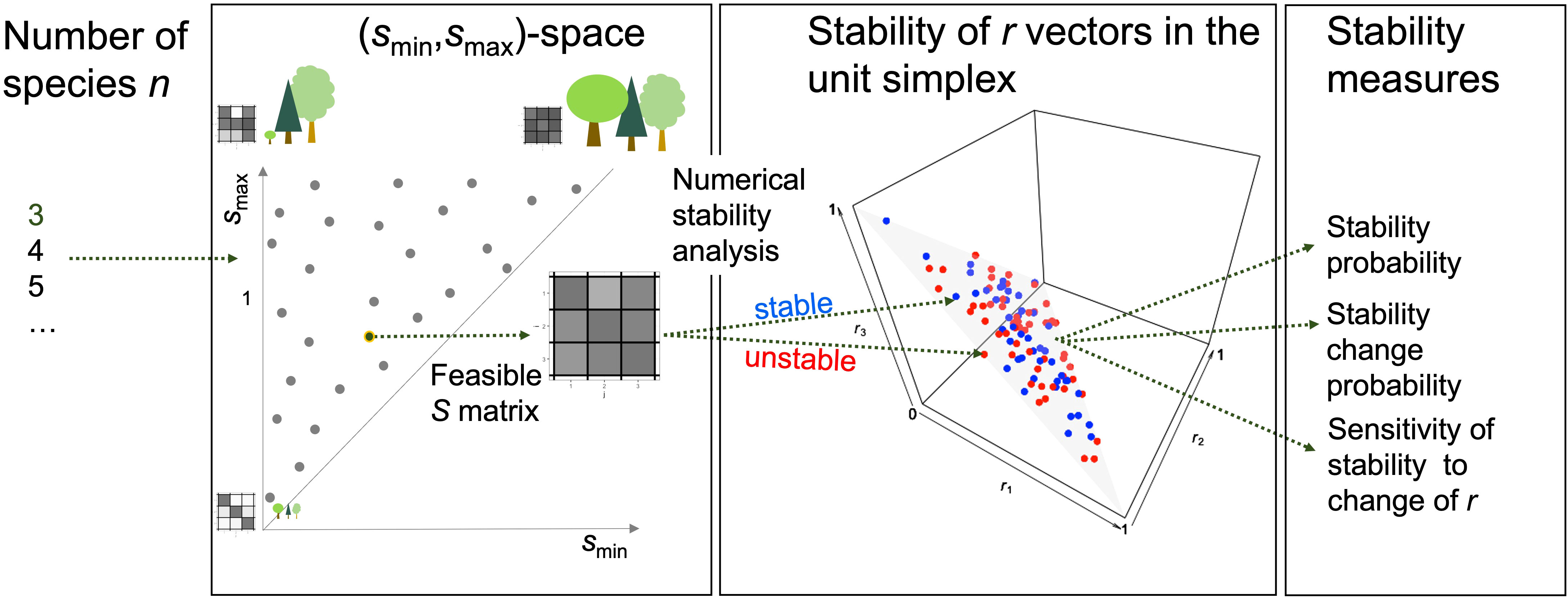
Figure 1 Overview over computational analysis of stability changes by the relative intrinsic growth rates r, demonstrated for the example n = 3. The analysis was repeated for different numbers n of species. For uniformly sampled points s in the (smin, smax)-space (short s-space), matrices S with smin ≤ sij ≤ smax were uniformly sampled. A point s stands for an infinite number of communities, each of which is characterized by its competition matrix S. The gray tones of the matrices and the tree sizes exemplify competition strengths. The sampling was repeated until a matrix S was feasible, i.e., all species had positive abundances at the equilibrium, or the maximal number of trials was reached. This matrix S was combined with m different relative intrinsic growth rate vectors r uniformly sampled from the unit simplex (r-space) (red and blue points on the gray triangle in the unit cube). The stability of the Lotka–Volterra competition model with matrix S and each sampled relative intrinsic growth rate vector r was determined by calculating the eigenvalues of its Jacobian matrix (blue points in the unit simplex are stable and red ones are unstable). Finally, three stability measures were calculated from the stability behavior in the unit simplex for the matrices S of points s = (smin, smax).
2.2 Numerical examinations
We studied the feasibility and stability by calculations in the s- and r-space (Figure 1). We used a numerical analysis framework (Figure 1, cf. Section 2.2.1) to investigate the feasibility (cf. Section 2.2.2) and the effects of changes in the intrinsic growth rate on the stability of the feasible matrices of the s-space (cf. Sections 2.2.1–2.2.5). In addition, the results were analyzed using different statistical measures in different reference regions of the s-space (cf. Sections 2.2.6–2.2.11) and against the number of species (cf. Section 2.2.9).
2.2.1 Randomly generated S matrices
The values smin and smax, determining the range of competition strengths in a community, were uniformly sampled (i.e., randomly sampled from a uniform distribution) in the s-space (Figure 1) within specified regions. The results of the analyses were visualized in the (smin, smax)-plane. For every point s = (smin, smax), the elements sij of the matrix S were uniformly sampled between smin and smax, with one sij = smin and one skl = smax for off-diagonal positions in the matrix. The intra-specific coefficients on the diagonal were set to sii = 1. Every point s = (smin, smax) defines infinitely many matrices S and the generation of S matrices stopped with the first feasible matrix found, i.e., one which defines a feasible solution z* of the LVC model, or when reaching a predefined maximum number of trials to avoid endless loops (cf. Section 2.2.2).
2.2.2 Probability of feasibility
Since feasibility of the S matrices is a prerequisite for the investigations of stability change, we examined how likely it is to find a feasible matrix in the s-space (cf. Figure 2 and S1). Testing the feasibility of uniformly sampled matrices S of a point s = (smin, smax) is a Bernoulli experiment, i.e., the number of trials of finding the first feasible S follows a geometric distribution. Thus, if the probability of finding a feasible matrix of a point s = (smin, smax) is pf,s, then the mean number of trials required is (Ibe, 2013). Per point s, the sampling rate for finding a feasible matrix is an estimator for pf,s. Thereby, is the number of sampled S matrices and is the found number of feasible ones. To ensure that the estimator satisfies a certain accuracy, was iteratively increased until converged, i.e., the last two estimations and differed by less than the absolute εabs and relative εrel thresholds, i.e., and . With this probability estimator value , the minimum number of trials required to find the first feasible matrix S is , i.e., (if ). The number was used as the upper limit in further simulations to find a feasible S matrix (cf. Section 2.2.1) with the predefined accuracy. This setup was limited by computational power to n = 17 for the chosen 30,000 s points in the chosen region.
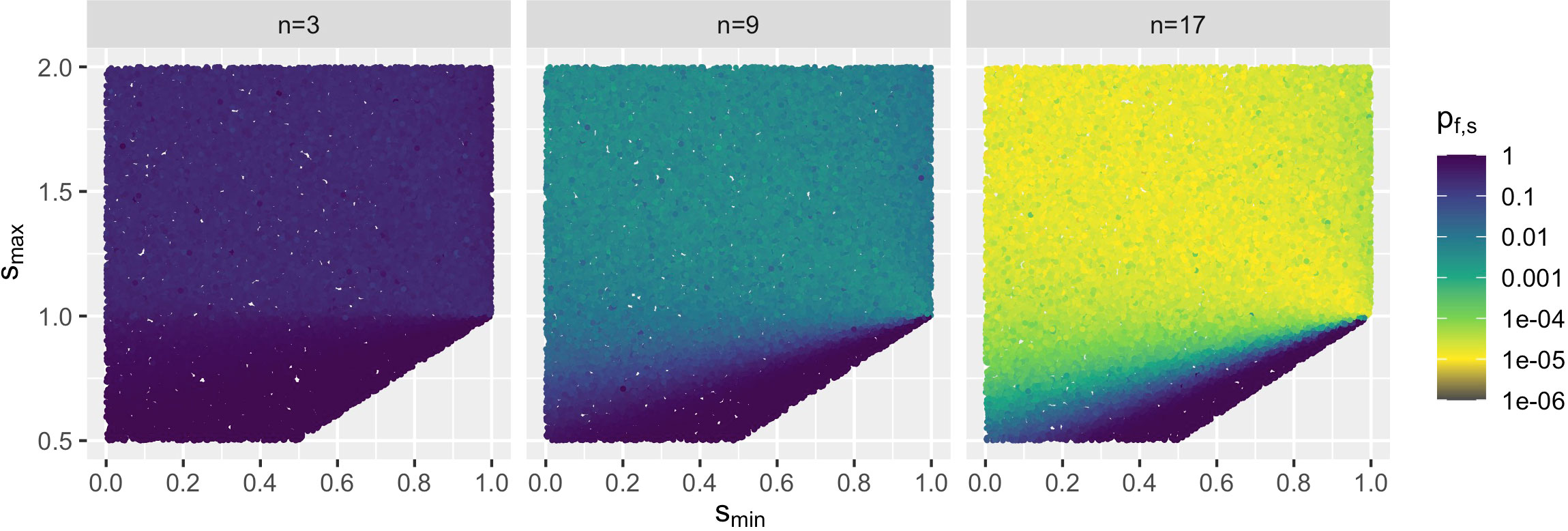
Figure 2 Examples of probability pf,s of finding a feasible matrix S of s = (smin, smax) points with smin ≤ sij ≤ smax for a selected number of species n by a Bernoulli experiment (cf. Section 2.2.2). In the chosen range, for all simulated n, 30,000 s points were uniformly sampled. The probability of finding a feasible matrix decreased with increasing the number n of species, but remained high in the bottom triangle Dn (cf. Section 2.2.8).
2.2.3 Changeable stability
At each point s = (smin, smax), m = 1,000 relative intrinsic growth rates vectors r ∈ Δn−1 were uniformly sampled from the r-space and the eigenvalues of the LVC model consisting of the matrix S and each r vector were calculated to determine (in)stability by determining numerically the eigenvalues of the Jacobian J (Eq. 3). Different stabilities for different r vectors mark then a stability change with r. Points s = (smin, smax) that change their stability with r will be referred to as changeable stability points below.
2.2.4 Triangle Tn of changeable stability
Changeable stability points occurred only in a triangular region Tn of the s-space, for each number n of species (cf. green lines in Figures 3, 4; Figures S2–S4). Outside Tn, the examined points were either always unstable or always stable. These triangles Tn are determined by the points (1, 1), (0, smax,u,n), and (0, smax,l,n), where smax,u,n (smax,l,n) is the maximum (minimum) intersection point on the smax-axis (i.e., intercept) of all lines through (1,1) and each s-point (smin,i,n, smax,i,n) with changeable stability. Describing such a line as linear equation by smax=b smin+a and inserting the point (1,1) results a=1-b, thus smax = b smin+1-b and therefore . For a given line through a point (smin,i,n, smax,i,n), it is and . The intercept is at smin = 0 and its value is therefore ai. Finally, the value is the highest and the lowest intercept.
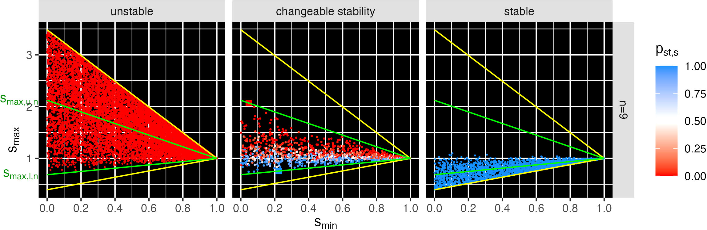
Figure 3 Example for n = 9 of stability probability pst,s over 1,000 different relative intrinsic growth rate vectors rk (0 means always unstable and 1 always stable) of feasible LVC model at points s = (smin, smax). Center: The found points with changeable stability are in the triangle T9, which is delimited by the green lines through the point s = (1, 1) and through the points with the maximum and minimum slope (larger red and blue dot). The values smax,u,n and smax,l,n are the intercepts of the green lines at the smin = 0 axis. The search range (yellow delimited triangle) was chosen heuristically slightly larger than the triangle T8 to ensure that points with changeable stability were not overlooked. Left: purely unstable; right: purely stable s points. In T9, the region with the changeable stability overlaps with the regions of purely unstable points above and purely stable points below. For all simulated n, cf. Figures S2–S4.
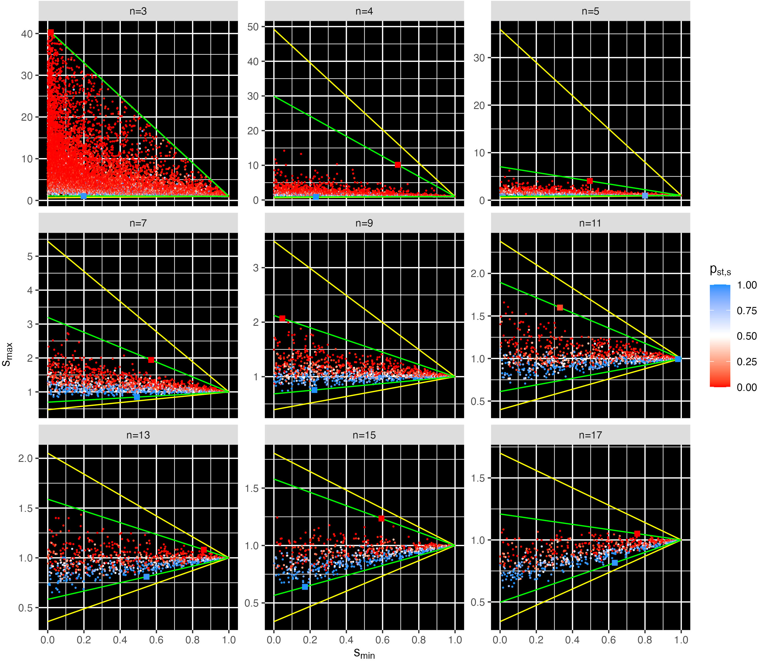
Figure 4 Points s = (smin, smax) with changeable stability for selected n, with the stability probability pst,s over 1,000 different relative intrinsic growth rate vectors rk. All points with changeable stability were in the triangles Tn that are delimited by the green lines through the point s = (1, 1) and through the points with the maximum and minimum slope (two larger dots per panel). The values smax,u,n and smax,l,n are the intercepts of the green lines at the smin = 0 axis. The search range (yellow delimited triangle) was heuristically chosen slightly larger than the triangle Tn−1 to ensure that points with changeable stability were not overlooked. For n = 3, the simulation range was heuristically chosen large. Note that the scale for smax differs in the panels. For all simulated n, cf. Figure S2.
2.2.5 Adaptive sampling region
Since the research topic of changeble stability is limited to the regions Tn, examinations can be restriced to Tn, to minimize the computational effort. Since the triangular regions Tn (cf. green lines in Figures 3 and 4, and Figures S2–S4) change with n, we determined iteratively search regions around Tn. Starting for n = 3 with smax = [0, 40], the first region T3 was chosen arbitrarily large for the changeable stability search. To determine the search region for changeable stability for the current n, the green triangle Tn−1 of the last iteration was used. It was heuristically (based on the pre-studies) extended by multiplying the upper and lower intercepts smax,u,n−1 and smax,l,n−1 (cf. Section 2.2.4) with 1.2 and 0.6, respectively, to ensure no changeable stability points were missed. These search regions are the yellow triangles in Figures 3 and 4 and Figures S2–S4. This reduced the computational effort required to find enough points of changeable stability and allowed to study changeable stability for up to n = 23 species on a computer cluster.
2.2.6 Stability change probability
As probability with which a point s changes its stability, we calculated the mean of the stability states over all r vectors at that point. The (in)stability of an LVC model with rτ ∈ Δn−1 and matrix S was recorded by στ = 1 for stability and στ = 0 for instability. The mean value is the probability of the LVC model to be stable. pst,s = 1 means always stable, pst,s = 0 means always unstable, and 0< pst,s< 1 means changeable stability. The value is then the probability that a stability change occurs at all.
2.2.7 Mean probability of stability change
To assess the influence of the community size n on the stability behavior, we wanted to know the mean probability of a stability change in the region Tn and for any larger region containing Tn. Within the triangle Tn, we calculated the mean probability of a stability change over all kn examined s points as . Then, the expected value of the number of changeable stability points in Tn is with area of Tn, sample density ρ, and consequently sample size . In an arbitrary reference region with area Aref, which contains Tn, the sample size is Arefρ and the expected value of the number of changeable stability points is , which is the same as because changeable stability only happens in Tn. Therefore, the mean probability of a stability change over all kn examined s points in Aref is = . We see that depends on n via and and inverse linearly on Aref. In the evaluation (cf. Figure 5), we used , i.e., the n dependent part, from which can be calculated for any reference region by dividing through Aref.
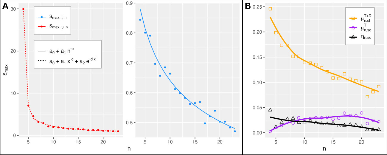
Figure 5 Changeable stability over n (4 ≤ n ≤ 23). (A) Functions of n that fit best (Table S1) the upper intercepts smax,u,n (left) and lower intercepts smax,l,n (right) of the boundaries of the changeable stability triangle Tn (green lines in Figures 3, 4, S2–S4) with the smin = 0 axis (fit by LOESS method; Hadley, 2016). (B) is the mean probability of a stability change in Tn. ηn,sc is the n dependent part of , the mean probability of stability change in a reference region of area Aref that contains Tn. is the mean probability of stability loss, i.e., that a point s in a stable state becomes unstable.
2.2.8 Mean probability of stability loss
Considering a community that is stable, but of which we know neither r nor s, we calculated the average probability that it will lose its stability if r changes. Such a stable community can be either located in the purely stable region of the s-space or in Tn, where it can be either purely or changeable stable. We looked first at a point s in Tn with changeable stability that is stable for a given r. The probability that this stable point changes to unstable is 1 − pst,s and the mean probability of such a stability loss in Tn is with kn,sc = |psc,s > 0| the number of all examined points with changeable stability. With kn (kn,st) as the number of all (always stable) s points in Tn, the fraction of the changeable stability points s in Tn is kn,sc/kn and that of changeable stability and always stable points s is (kn,sc + kn,st)/kn. Additionally, the triangle Dn below Tn down to the diagonal dmin=max := (smin = smax) (i.e., where smin = smax), which, according to the simulations contains only purely stable s points, has the area . Then, is the fraction of changeable stability points of all stable points. The mean probability that a stable point s loses its stability is then (cf. Figure 5).
2.2.9 Fit of axis intercepts of the lines of triangles Tn
To get a general idea of the change of the triangles’ Tn size and location in the s-space with increasing community size n, we approximated the intercepts smax,l,n and smax,u,n (cf. Section 2.2.4) by functions of n. To this aim, we determined these intercepts of the lower and upper lines of the triangles for each n. Then, we fitted these intercepts with different functions. Intercepts for n = 3 were excluded because the first simulation range was chosen by heuristic pre-studies. We chose the decreasing functions , , , , , , , and fitted them smax,l,n and smax,u,n by a nonlinear least squares fit (R Core Team, 2021), weighted with to emphasize higher n. Using the lowest value of the second-order Akaike Information Criterion (AICc) to test the quality of the fit (Barton, 2020), the best fitting function was chosen (cf. Table S1; Figure 5A).
2.2.10 Local sensitivity of stability to changes of r
Generally, the local sensitivity quantifies how an output variable responds to changes in a given (local) value of an input variable or parameter. This measure helps to interpret the effects of the arrangement of stable and unstable r points in r-space on stability changes. Here, the equilibrium of the LVC model is either stable (σν = 1) or unstable (σν = 0), and hence, its local sensitivity to changes in the relative intrinsic growth rate vectors rτ ∈ Δn−1 is (Pianosi et al., 2016). This can be aproximated by with the squared Euclidian distance (Spencer, 2014), which emphasizes the effect of short distance changes. Normalizing with the maximum possible local sensitivity , where all rν have a stability state other than rτ, the local sensitivity measure is with 0 ≤ γτ ≤ 1. The measure indicates how likely a change in stability is for a given rτ relative to all other r. The value of γτ depends on the location rτ ∈ Δn−1 and the distances dτν of the rν to rτ with a different stability state and is able to distinguish between different arragements of stable and unstable r vectors (cf. example in Figure S6). The γτ were grouped in n and pst,s classes and represented as frequency distributions (Figures 6, S5).
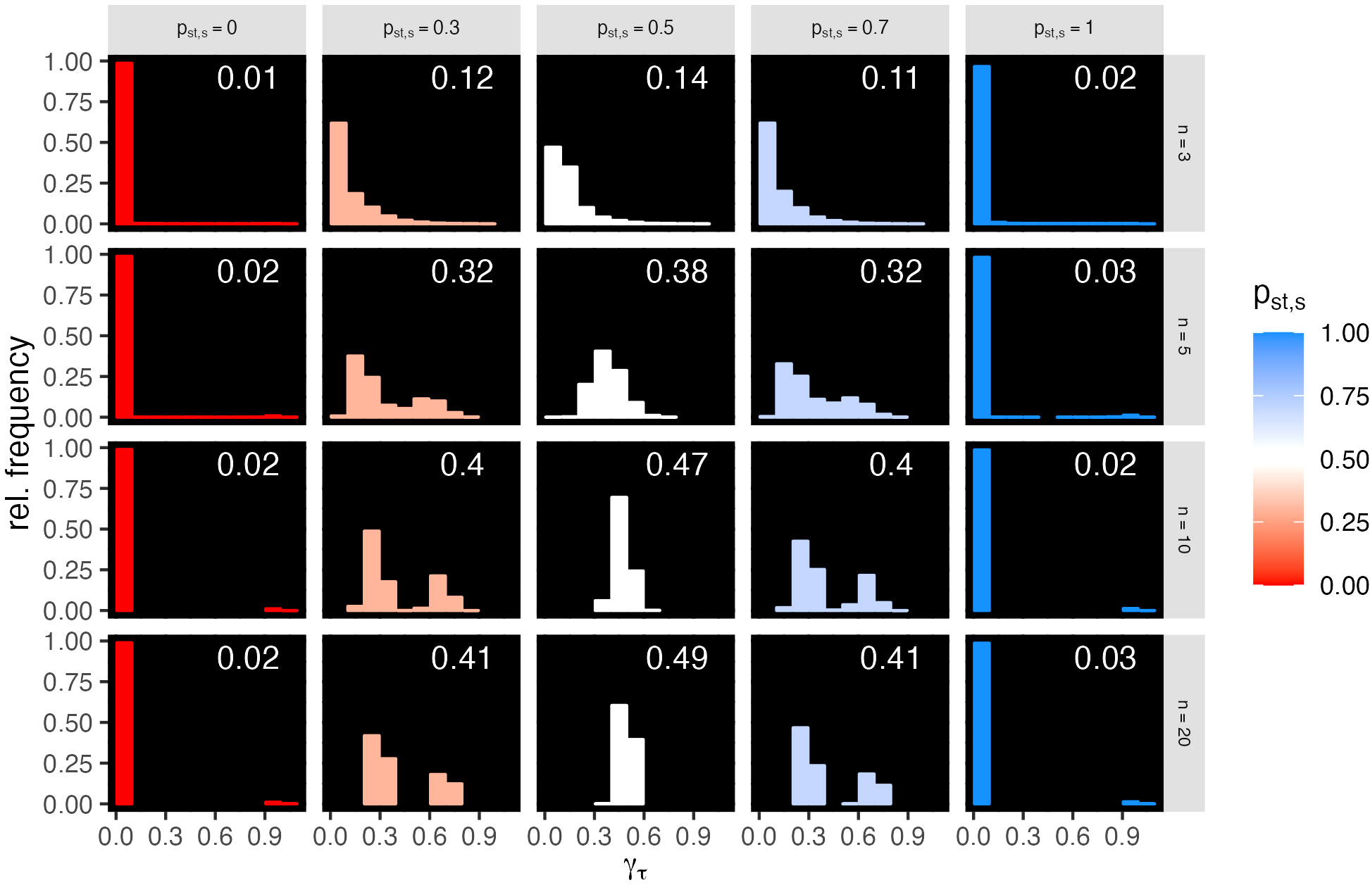
Figure 6 Examples of relative frequency distributions of local sensitivities γτ for all intrinsic growth rate rτ vectors of all changeable stability s = (smin, smax) points, for selected species numbers n = 3, 5, 10, and 20 (rows) and stability probabilities pst,s (columns are the means of classes of width 0.1). The white numbers are the means of γτ. For all n, cf. Figure S5.
2.2.11 Sensitivities for random and clustered arrangements of stable points
To get an idea about the spatial arrangements in Δn−1 of stable and unstable r vectors underlying the obtained frequency distributions of sensitivity γτ, we compared these frequency distributions to those generated from given spatial arrangements of stable and unstable points. To this aim, we generated random and clustered (in the center and in the corner of the simplex) spatial patterns of 10,000 points with different probabilities p of two states of red and blue points (Figure S6). Blue and red were interpreted as stable and unstable, respectively. The sensitivity measure γτ was applied to these arrangements for all n and p. Comparing the resulting distributions with the distributions of the sensitivities γτ to a change in r (Figure S5) with the Kolmogorov–Smirnov test statistic (R-function ks.test; R Core Team, 2021) revealed that the latter were most similar to the clustered distributions for n up to about n = 10 and to the random distributions for n > 10 (Figure S7).
3 Results
3.1 Theoretical results
The theoretical examinations show that (a) the equilibria z* and their feasibility are independent of the intrinsic growth rates (Eq. 1) and (b) the intrinsic growth rates of the extinct species cannot change the sign of the eigenvalues and therefore do not affect the stability of the equilibria (Eq. 2). The Jacobian matrix J of the surviving species contains the intrinsic growth rates that (c) have therefore an influence on the eigenvalues and the stability of the equilibria (Eq. 3). This influence on stability results (d) from the relative intrinsic growth rates ri, since the constant factor rc ∈ ℝ+ has no effect on the sign of the real part of the eigenvalues of J (Eq. 3).
3.2 Feasibility
We studied the feasibility by calculations in the s-space. Figure 2 and Figure S1 show the probabilities pf,s to find a feasible matrix S for points s = (smin, smax) with smin ≤ sij ≤ smax (cf. Section 2.2.2). Overall, the probability of finding a feasible matrix decreased with increasing the number n of species, but remained high in the bottom triangle close to the diagonal dmin=max (i.e., where smin = smax). For the studied n ≤ 17, each with 30,000 s points in the selected range, always a feasible matrix S was found with probability pf,s ≥ 10−6. Therefore, in all subsequent simulations, a maximum of random matrices S were generated to find a feasible one for each s point (cf. Section 2.2.1).
3.3 Stability
We used the numerical analysis framework (Figure 1, cf. 2.2) to investigate the effects of changes in the intrinsic growth rate on the stability of the feasible matrices of the s-space. In combination with heuristic pre-studies that identified interesting parameter ranges, the available computing capacity allowed a systematic numerical analysis for species numbers up to n = 23. The eigenvalues of the Jacobian J, which depends on the matrix S and the relative intrinsic growth rate vectors rk = (ri)k ∈ Δn−1, k = 1,…,1000, showed that, often, the LVC model for the same S matrix was stable for some rk vectors (stable r vectors) and unstable for others (unstable r vectors). In such cases, stability changes between some of the different rk vectors (changeable stability). Points s = (smin, smax) with changeable stability are located in triangles Tn (green lines through the point s = (1, 1) in Figures 3, 4 and Figures S2–S4). Figure 3 shows the example of a nine-species community (n = 9) with points that were unstable (left), had changeable stability (center), and were stable (right).
The points of changeable stability in Tn had a probability for feasibility higher than 10−4 (compare Figure 2 with Figure 4, and Figure S1 with Figure S2). The stability probability pst,s for points with changeable stability (Figures 3, 4, Figure S2) increased from close to 0 (red: unstable communities for almost all rk) to 0.5 (white: stable/instable communities for half of the rk each) to close to 1 (blue: stable communities for almost all rk). Consequently, the stability change probability psc,s (cf. Section 2.2.6) is 0 for nearly stable and instable s points, increasing to 1 at pst,s = 0.5. The triangles Tn with the changeable stability overlap with the regions of purely unstable points above and purely stable points below for all examined n (Figure 3 and Figures S2–S4). Thus, the points in the s-space represent communities that transition from unstable to changeable stability to stable as smax decreases. Figure 4 and Figure S2 show that with increasing n, Tn rotates counterclockwise and its area decreases, i.e., its upper and lower bounds smax,u,n and smax,l,n both decrease and approach each other.
3.4 Changeable stability depending on species number
Figure 5A shows the functions of the number of species (4 ≤ n ≤ 23) that best fit the smax,u,n and smax,l,n intercepts of Tn (Table S1, Section 2.2.9). As the number n of species increases, smax,u,n and smax,l,n decrease and approach each other. This corroborates that the region of Tn shrinks and rotates in the direction of the diagonal dmin=max (i.e., where smin = smax). Therefore, as the number of species increases, feasible and stable or stability changing competitive communities have more and more weaker and similar interactions smin ≤ sij ≤ smax. However, the coefficients a0 of the fits of different functions (Table S1) indicate that smax,u,n and smax,l,n possibly do not converge (a0 of smax,u,n > a0 of smax,l,n). Thus, for every n, there is possibly a non-empty Tn, which probably also contains purely stable communities. Since the fit qualities (AIC in Table S1) of the functions for smax,l,n were very similar, it is unclear whether a0 of smax,l,n is zero or positive, i.e., whether the region containing only stable points completely coincides to dmin=max for large n. Figure 5B shows that the mean probability (cf. Section 2.2.7) of an r-induced stability change in Tn ranges between close to 0 and 4%. ηn,sc, the n-dependent part of the mean probability of stability change in a reference region of area Aref that includes Tn, is of the same order of magnitude and decreases linearly with n. can be calculated for any reference region by dividing ηn,sc through Aref (cf. Section 2.2.7). In the region Dn between Tn and the dmin=max diagonal, all s points are purely stable. With the lower boundary of Tn turning in the direction of the diagonal, Dn also becomes smaller. In the shrinking combined region of pure and changeable stability (Dn and Tn), the mean probability of a (changeable or purely) stable point to become unstable starts at 0.25 and decreases to approximately 0.075 with increasing n (cf. Section 2.2.8).
3.5 Sensitivity of changeable stability to intrinsic growth rate
We determined how sensitive the stability of each changeable stability point s = (smin, smax) is to distances from each vector rτ to all other vectors rk ∈ Δn−1 (cf. Section 2.2.10). These distances indicate how much rτ must be changed to move the LVC model to another stability state. We calculated the relative frequency distribution of the local sensitivity measure γτ (cf. Section 2.2.10) over all s points in combined classes of stability probability pst,s and n (panels in Figures 6; S5). The mean sensitivity (white numbers, Figures 6; S5) increases with n up to 0.49 and is highest for pst,s = 0.5. For pst,s close to 0 and 1, γτ is very high for a few rτ and very low for most rτ (left-skewed). With pst,s at 0.3 and 0.7, γτ is either low or high (bimodal), and with pst,s at 0.5, the distribution of γτ is unimodal. For large n, the peaks of the distribution are narrow, while for small n, they are broader and more left-skewed. Comparison with the pattern resulting from random and clustered spatial arrangements (cf. example in Figure S6) indicates that the arrangement of the stable r vectors in the r-space is close to random for large n and close to clustered for small n (Figure S7). The s points with a stability probability pst,s approximately 0.5 in the center of the triangle Tn (white points in Figures 3, 4; S2) are in average most sensitive to changes in r (white numbers in the panels, Figure 6 and Figure S5), and the single relatively narrow peaks imply that the sensitivity γτ is similar for all r. However, for s points with pst,s at 0.3 (0.7) bordering the center of Tn (light blue and light red points in Figures 3, 4; S2), the average sensitivity is smaller and the bimodality implies that the sensitivity to changes in r is different over the r-space.
4 Discussion
In our MCT formulation of the LVC model, a community is represented by the combination of the competition matrix S and the intrinsic growth rate vector r. The matrix S determines the composition of species at equilibrium and, together with r, the trajectory leading to that equilibrium. A change in the stability of the equilibrium implies a change in the composition of the community and of its dynamics. Gain of stability sets in motion the assembly of a new community, with species provided, e.g., by immigration. Loss of stability means that a community that is on its way to or already in a stable equilibrium moves away from it and toward another stable equilibrium with different species (Chesson, 2018). Such a loss has different consequences in real systems ranging from subtle changes to regime shifts (Scheffer and Carpenter, 2003). It can mean the replacement of a few species by other species up to the complete exchange of a community, or the loss of a few species up to mass extinction (Reyer et al., 2015).
Our results show that community stability can be altered by changes in the relative intrinsic growth rates of species. However, this only happens within a certain range of competitive strengths.
Changes in relative intrinsic growth rates, like other aspects of community dynamics, can be caused by many processes or drivers. Such drivers, including temporal or spatial environmental changes [e.g., in climate (Louthan and Morris, 2021; Usinowicz and Levine, 2021), nutrients (Griffiths et al., 2015), sediments (Sahade et al., 2015), and pathogens (Mordecai, 2011; Metz et al., 2012)] and human activities [e.g., climate change, selective harvesting (Turkalo et al., 2017)], that affect species differently can trigger a change in a community from stable to unstable or vice versa. Consequently, even a change in the r of a single species can change the stability of an entire community. Even if the environment remains the same, the relative intrinsic growth rates r change when, in a community, species go extinct or new species are added by introduction, invasion, or evolution (Munson and Lauenroth, 2009; Gioria et al., 2018; Linders et al., 2019).
As long as the equilibrium of the community remains stable, i.e., a tipping point has not yet been reached, a changing r does not affect the composition of the community at equilibrium, which therefore does not provide an early warning sign of a change in stability (Boerlijst et al., 2013). On the other hand, if the community is not in equilibrium, a change in r will affect species abundances and dynamics, which could be used as an early warning sign. For example, different recovery rates under different r after perturbations can be such an early warning sign (Munson and Lauenroth, 2009; Gioria et al., 2018; Brondizio et al., 2019; Linders et al., 2019). At the tipping point, the stability changes abruptly, but the inertia of a real system can cause it to take some time to reach a new stable equilibrium. (Lloret et al., 2012).
In detail, our results show that positive intrinsic growth rates of species do not affect species composition, abundances, and community feasibility (Chesson, 2018), but that they can affect community stability when there are at least three species. Thereby, the intrinsic growth rates of extinct species have no influence on the stability of equilibria (Chesson, 2018). However, the relative intrinsic growth rates of the surviving species influence the stability and thus their coexistence. Interestingly, in the permanence theory, which takes a different view on stable coexistence, the intrinsic growth rates of species in an equilibrium do not matter (Chesson, 2018). Studies using the LVC model in the r-formalism have also shown that intrinsic growth rates influence not only community stability but also the feasibility (Saavedra et al., 2017; Saavedra et al., 2020; Song et al., 2021; Selaković et al., 2022). Our results show that it is the relative values of intrinsic growth rates that affect the stability of a community. This is consistent with results of the r-formalism LVC model that it is sufficient to use normalized r vectors as a measure of structural stability (Grilli et al., 2017). Any influence that alters relative intrinsic growth rates and affects species differently can trigger a change in a community from stable to unstable or vice versa, i.e., a tipping point is crossed. Consequently, even a change in the r of a single species can change the stability of an entire community.
Our approach to determine the sensitivity has a similarity to the structural stability approach in that it combines feasibility and stability depending on parameter ranges (Rohr et al., 2014; Grilli et al., 2017). However, it is less restrictive as it considers arbitrary competition matrices and thus community compositions and applies the general Lyapunov stability criterion (Logofet, 2005). The local sensitivity used represents the risk that a change in r will move a community to a different stability state, emphasizing small changes in r that are assumed to be more likely. We found that the mean local sensitivity increases with community size and is highest in the center part of Tn, where also stability change probability psc,s is the highest. The sensitivity of a community is not homogeneously distributed in r-space (Grilli et al., 2017) and therefore depends on the position of the community in r-space. That means, local sensitivity can be similar but also highly different for communities with the same interaction matrices but different r vectors. Overall, there is a non-negligible risk that already a small environmental change affecting r can trigger a stability change.
Each point s = (smin, smax) represents an infinite number of competition matrices S, one of which was selected that allowed a feasible community. For all species numbers studied, the points s with changeable stability are in a region Tn between and overlapping with the regions of completely unstable and completely stable points. As smax in Tn decreases, there are more and more relative intrinsic growth rates for which the communities are stable and at the same time the probability of a stability change first increases and then decreases again. The region Tn shrinks as species numbers n increase and approaches the diagonal dmin=max, implying that the competition strengths sij of the communities become smaller and more similar. The mean probability of a community uniformly sampled in Tn to change its (in)stability is less than 4% independent of n. The mean probability of a stability change in a reference region (which includes Tn), decreases with n and also with increasing the reference region. Thus, the larger the reference region, the less frequently a changeable stability community is found by random sampling. However, the mean probability of a given stable community—that is necessarily either purely or changeable stable with a stable r vector—to become unstable is between 25% and 8% and decreases with n (cf. Figure 5B). This risk of stability loss is not negligible, but species-rich communities are less susceptible to it than species-poor ones (De Boeck et al., 2018). Additionally, a change in intrinsic growth rates is much more likely to cause a stable community to lose its stability than a community randomly selected in an arbitrary region to change its stability. Because stable communities are in restricted regions (Tn and Dn) whose sizes decrease with n, they are difficult to hit by random sampling in any larger region, in particular for large communities, which contributes to the stability–diversity debate (Gardner and Ashby, 1970; May, 1972; Goh and Jennings, 1977; McCann, 2000). Additionally, the regions with (changeable) stability are located where the probability of feasibility is high. This is in accordance to the results of the structural stability approach (May, 1972), where feasibility implies stability, that “the larger the system is, the smaller is the set of conditions leading to coexistence” (Grilli et al., 2017). However, the fits of the intercepts of the changeable stability regions suggest that feasible and stable randomly assembled matrices exist even for high n, similarly to previous findings (Serván et al., 2018). This provides a new aspect to the theoretical explanation for the existence of species-rich competing communities (Hutchinson, 1961; Chesson, 2000; Li and Chesson, 2016; Saavedra et al., 2017; Schreiber et al., 2023).
Data availability statement
The original contributions presented in the study are included in the article/Supplementary Material. Further inquiries can be directed to the corresponding author.
Author contributions
TL and HL contributed equally to this work and share first authorship. All authors contributed to the article and approved the submitted version.
Funding
Open access funding by ETH Zurich.
Conflict of interest
The authors declare that the research was conducted in the absence of any commercial or financial relationships that could be construed as a potential conflict of interest.
Publisher’s note
All claims expressed in this article are solely those of the authors and do not necessarily represent those of their affiliated organizations, or those of the publisher, the editors and the reviewers. Any product that may be evaluated in this article, or claim that may be made by its manufacturer, is not guaranteed or endorsed by the publisher.
Supplementary material
The Supplementary Material for this article can be found online at: https://www.frontiersin.org/articles/10.3389/fevo.2023.1202022/full#supplementary-material
References
Adler P. B., Smull D., Beard K. H., Choi R. T., Furniss T., Kulmatiski A., et al. (2018). Competition and coexistence in plant communities: intraspecific competition is stronger than interspecific competition. Ecol. Lett. 21 (9), 1319–1329. doi: 10.1111/ele.13098
Allesina S., Levine J. M. (2011). A competitive network theory of species diversity. PNAS Proc. Natl. Acad. Sci. United States America 108 (14), 5638–5642. doi: 10.1073/pnas.1014428108
Allesina S., Tang S. (2012). Stability criteria for complex ecosystems. Nature 483 (7388), 205–208. doi: 10.1038/nature10832
Barton K. (2020). “MuMIn: multi-model inference” (R package version 1) Available at: https://cran.r-project.org/web/packages/MuMIn.
Bauman D., Fortunel C., Cernusak L. A., Bentley L. P., McMahon S. M., Rifai S. W., et al. (2022). Tropical tree growth sensitivity to climate is driven by species intrinsic growth rate and leaf traits. Global Change Biol. 28 (4), 1414–1432. doi: 10.1111/gcb.15982
Beisner B. E., Haydon D. T., Cuddington K. (2003). Alternative stable states in ecology. Front. Ecol. Environ. 1 (7), 376–382. doi: 10.2307/3868190
Bland L. M., Watermeyer K. E., Keith D. A., Nicholson E., Regan T. J., Shannon L. J. (2018). Assessing risks to marine ecosystems with indicators, ecosystem models and experts. Biol. Conserv. 227, 19–28. doi: 10.1016/j.biocon.2018.08.019
Boerlijst M. C., Oudman T., de Roos A. M. (2013). Catastrophic collapse can occur without early warning: examples of silent catastrophes in structured ecological models. PloS One 8 (4), e62033. doi: 10.1371/journal.pone.0062033
Brondizio E. S., Settele J., Díaz S., Ngo H. T. (2019). IPBES 2019: global assessment report on biodiversity and ecosystem services of the intergovernmental science-policy platform on biodiversity and ecosystem services. IPBES Secretariat: Bonn, Germany.
Campbell C., Russo L., Albert R., Buckling A., Shea K. (2022). Whole community invasions and the integration of novel ecosystems. PloS Comput. Biol. 18 (6), 1-20. doi: 10.1371/journal.pcbi.1010151
Case T. J. (1995). Surprising behavior from a familiar model and implications for competition theory. Am. Nat. 146 (6), 961–966. doi: 10.1086/285834
Chesson P. (2000). Mechanisms of maintenance of species diversity. Annu. Rev. Ecol. Systematics 31, 343–366. doi: 10.1146/annurev.ecolsys.31.1.343
Chesson P. (2018). Updates on mechanisms of maintenance of species diversity. J. Ecol. 106 (5), 1773–1794. doi: 10.1111/1365-2745.13035
Dakos V., Matthews B., Hendry A. P., Levine J., Loeuille N., Norberg J., et al. (2019). Ecosystem tipping points in an evolving world. Nat. Ecol. Evol. 3 (3), 355–362. doi: 10.1038/s41559-019-0797-2
De Boeck H. J., Bloor J. M. G., Kreyling J., Ransijn J. C. G., Nijs I., Jentsch A., et al. (2018). Patterns and drivers of biodiversity–stability relationships under climate extremes. J. Ecol. 106 (3), 890–902. doi: 10.1111/1365-2745.12897
Fort H. (2020). “Lotka–Volterra models for multispecies communities and their usefulness as quantitative predicting tools,” in Ecological modelling and ecophysics. Ed. Fort H. (Bristol, UK: IOP Publishing), 1–35.
Fried Y., Shnerb N. M., Kessler D. A. (2017). Alternative steady states in ecological networks. Phys. Rev. E 96 (1), 012412. doi: 10.1103/PhysRevE.96.012412
Gamelon M., Sandercock B. K., Sæther B.-E. (2019). Does harvesting amplify environmentally induced population fluctuations over time in marine and terrestrial species? J. Appl. Ecol. 56 (9), 2186–2194. doi: 10.1111/1365-2664.13466
Gardner M. R., Ashby W. R. (1970). Connectance of large dynamic (Cybernetic) systems: critical values for stability. Nature 228 (5273), 784–784. doi: 1038/228784a0
Gause G. F. (1932). Experimental studies on the struggle for existence: I. Mixed population of two species of yeast. J. Exp. Biol. 9 (4), 389–402. doi: 10.1242/jeb.9.4.389
Gioria M., O’Flynn C., Osborne B. A. (2018). A review of the impacts of major terrestrial invasive alien plants in Ireland. Biol. Environment: Proc. R. Irish Acad. 118B (3), 157–179. doi: 10.3318/bioe.2018.15
Goh B. S. (1978). Sector stability of a complex ecosystem model. Math. Biosci. 40 (1-2), 157–166. doi: 10.1016/0025-5564(78)90078-0
Goh B. S., Jennings L. S. (1977). Feasibility and stability in randomly assembled Lotka-Volterra models. Ecol. Model. 3, 63–71. doi: 10.1016/0304-3800(77)90024-2
Griffiths J. I., Warren P. H., Childs D. Z. (2015). Multiple environmental changes interact to modify species dynamics and invasion rates. Oikos 124 (4), 458–468. doi: 10.1111/oik.01704
Grilli J., Adorisio M., Suweis S., Barabas G., Banavar J. R., Allesina S., et al. (2017). Feasibility and coexistence of large ecological communities. Nat. Commun. 8, 1-8. doi: 10.1038/ncomms14389
Hansen B. B., Gamelon M., Albon S. D., Lee A. M., Stien A., Irvine R. J., et al. (2019). More frequent extreme climate events stabilize reindeer population dynamics. Nat. Commun. 10 (1), 1616. doi: 10.1038/s41467-019-09332-5
Heymans J. J., Tomczak M. T. (2016). Regime shifts in the Northern Benguela ecosystem: Challenges for management. Ecol. Model. 331, 151–159. doi: 10.1016/j.ecolmodel.2015.10.027
Hutchinson G. E. (1961). The paradox of the plankton. Am. Nat. 95 (882), 137–145. doi: 10.1086/282171
Kareiva P., Carranza V. (2018). Existential risk due to ecosystem collapse: Nature strikes back. Futures 102, 39–50. doi: 10.1016/j.futures.2018.01.001
Kessler D. A., Shnerb N. M. (2015). Generalized model of island biodiversity. Phys. Rev. E 91 (4), 042705-1–042705-11. doi: 10.1103/PhysRevE.91.042705
Li L., Chesson P. (2016). The effects of dynamical rates on species coexistence in a variable environment: the paradox of the plankton revisited. Am. Nat. 188 (2), E46–E58. doi: 10.1086/687111
Liautaud K., van Nes E. H., Barbier M., Scheffer M., Loreau M. (2019). Superorganisms or loose collections of species? A unifying theory of community patterns along environmental gradients. Ecol. Lett. 22 (8), 1243–1252. doi: 10.1111/ele.13289
Linders T. E. W., Schaffner U., Eschen R., Abebe A., Choge S. K., Nigatu L., et al. (2019). Direct and indirect effects of invasive species: Biodiversity loss is a major mechanism by which an invasive tree affects ecosystem functioning. J. Ecol. 107 (6), 2660–2672. doi: 10.1111/1365-2745.13268
Lischke H., Löffler T. J. (2017). Finding all multiple stable fixpoints of n-species Lotka-Volterra competition models. Theor. Population Biol. 115 (June 017), 24–34. doi: 10.1016/j.tpb.2017.02.001
Lloret F., Escudero A., Iriondo J. M., Martinez-Vilalta J., Valladares F. (2012). Extreme climatic events and vegetation: the role of stabilizing processes. Global Change Biol. 18 (3), 797–805. doi: 10.1111/j.1365-2486.2011.02624.x
Logofet D. O. (2005). Stronger-than-Lyapunov notions of matrix stability, or how “flowers” help solve problems in mathematical ecology. Linear Algebra Its Appl. 398, 75–100. doi: 10.1016/j.laa.2003.04.001
Louthan A. M., Morris W. (2021). Climate change impacts on population growth across a species’ range differ due to nonlinear responses of populations to climate and variation in rates of climate change. PloS One 16 (3), e0247290. doi: 10.1371/journal.pone.0247290
May R. M. (1972). Will a large complex system be stable? Nature 238 (5364), 413–414. doi: 10.1038/238413a0
McCann K. S. (2000). The diversity-stability debate. Nature 405 (6783), 228–233. doi: 10.1038/35012234
Mieth A., Bork H. -R. (2010). Humans, climate or introduced rats – which is to blame for the woodland destruction on prehistoric Rapa Nui (Easter Island)? J. Archaeol. Sci. 37, 417–426. doi: 10.1016/j.jas.2009.10.00
Metz M. R., Frangioso K. M., Wickland A. C., Meentemeyer R. K., Rizzo D. M. (2012). An emergent disease causes directional changes in forest species composition in coastal California. Ecosphere 3 (10), 1-23. doi: 10.1890/Es12-00107.1
Mordecai E. A. (2011). Pathogen impacts on plant communities: unifying theory, concepts, and empirical work. Ecol. Monogr. 81 (3), 429–441. doi: 10.1890/10-2241.1
Munson S. M., Lauenroth W. K. (2009). Plant population and community responses to removal of dominant species in the shortgrass steppe. J. Vegetation Sci. 20 (2), 224–232. doi: 10.1111/j.1654-1103.2009.05556.x
Pianosi F., Beven K., Freer J., Hall J. W., Rougier J., Stephenson D. B., et al. (2016). Sensitivity analysis of environmental models: A systematic review with practical workflow. Environ. Model. Software 79, 214–232. doi: 10.1016/j.envsoft.2016.02.008
R Core Team. (2021). R: A language and environment for statistical computing (Vienna, Austria: R Foundation for Statistical Computing).
Reyer C. P. O., Rammig A., Brouwers N., Langerwisch F. (2015). Forest resilience, tipping points and global change processes. J. Ecol. 103 (1), 1–4. doi: 10.1111/1365-2745.12342
Rohr R. P., Saavedra S., Bascompte J. (2014). On the structural stability of mutualistic systems. Science 345 (6195), 1–9. doi: 10.1126/science.1253497
Saavedra S., Medeiros L. P., AlAdwani M. (2020). Structural forecasting of species persistence under changing environments. Ecol. Lett. 23 (10), 1511–1521. doi: 10.1111/ele.13582
Saavedra S., Rohr R. P., Bascompte J., Godoy O., Kraft N. J. B., Levine J. M. (2017). A structural approach for understanding multispecies coexistence. Ecol. Monogr. 87 (3), 470–486. doi: 10.1002/ecm.1263
Sahade R., Lagger C., Torre L., Momo F., Monien P., Schloss I., et al. (2015). Climate change and glacier retreat drive shifts in an Antarctic benthic ecosystem. Sci. Adv. 1 (10), 1–8. doi: 10.1126/sciadv.1500050
Scheffer M., Carpenter S. R. (2003). Catastrophic regime shifts in ecosystems: linking theory to observation. Trends Ecol. Evol. 18 (12), 648–656. doi: 10.1016/j.tree.2003.09.002
Schreiber S. J., Levine J. M., Godoy O., Kraft N. J. B., Hart S. P. (2023). Does deterministic coexistence theory matter in a finite world? Ecology 104 (1), e3838. doi: 10.1002/ecy.3838
Selaković S., Säterberg T., Heesterbeek H. (2022). Ecological impact of changes in intrinsic growth rates of species at different trophic levels. Oikos 2022 (4), e08712. doi: 10.1111/oik.08712
Serván C. A., Capitán J. A., Grilli J., Morrison K. E., Allesina S. (2018). Coexistence of many species in random ecosystems. Nat. Ecol. Evol. 2 (8), 1237–1242. doi: 10.1038/s41559-018-0603-6
Song C. L., Rohr R. P., Vasseur D., Saavedra S. (2020). Disentangling the effects of external perturbations on coexistence and priority effects. J. Ecol. 108 (4), 1677–1689. doi: 10.1111/1365-2745.13349
Song C. L., Saavedra S. (2018). Will a small randomly assembled community be feasible and stable? Ecology 99 (3), 743–751. doi: 10.1002/ecy.2125
Song C. L., Uricchio L. H., Mordecai E. A., Saavedra S. (2021). Understanding the emergence of contingent and deterministic exclusion in multispecies communities. Ecol. Lett. 24 (10), 2155–2168. doi: 10.1111/ele.13846
Spencer N. H. (2014). Essentials of multivariate data analysis (Boca Raton, London, New York: Chapman and Hall).
Stinson K. A., Campbell S. A., Powell J. R., Wolfe B. E., Callaway R. M., Thelen G. C., et al. (2006). Invasive plant suppresses the growth of native tree seedlings by disrupting belowground mutualisms. PloS Biol. 4 (5), 727-731. doi: 10.1371/journal.pbio.0040140
Tabi A., Pennekamp F., Altermatt F., Alther R., Fronhofer E. A., Horgan K., et al. (2020). Species multidimensional effects explain idiosyncratic responses of communities to environmental change. Nat. Ecol. Evol. 4 (8), 1036–1043. doi: 10.1038/s41559-020-1206-6
Turkalo A. K., Wrege P. H., Wittemyer G. (2017). Slow intrinsic growth rate in forest elephants indicates recovery from poaching will require decades. J. Appl. Ecol. 54 (1), 153–159. doi: 10.1111/1365-2664.12764
Keywords: Lotka–Volterra competition model, relative intrinsic growth rate, community stability, stability change, feasibility
Citation: Löffler TJ and Lischke H (2023) Changing relative intrinsic growth rates of species alter the stability of species communities. Front. Ecol. Evol. 11:1202022. doi: 10.3389/fevo.2023.1202022
Received: 07 April 2023; Accepted: 27 September 2023;
Published: 16 October 2023.
Edited by:
Pavel Kindlmann, Charles University, CzechiaReviewed by:
Sourav Kumar Sasmal, Indian Institute of Technology Roorkee, IndiaJan Alfred Freund, University of Oldenburg, Germany
Copyright © 2023 Löffler and Lischke. This is an open-access article distributed under the terms of the Creative Commons Attribution License (CC BY). The use, distribution or reproduction in other forums is permitted, provided the original author(s) and the copyright owner(s) are credited and that the original publication in this journal is cited, in accordance with accepted academic practice. No use, distribution or reproduction is permitted which does not comply with these terms.
*Correspondence: Thomas J. Löffler, bG90aG9tYXNAZXRoei5jaA==; dGhvbWFzLmxvZWZmbGVyQHdzbC5jaA==
†These authors have contributed equally to this work and share first authorship