The noise is the signal: spatio-temporal variability of production and productivity in high elevation meadows in the Sierra Nevada mountain range of North America

There are expectations that increasing temperatures will lead to significant changes in structure and function of montane meadows, including greater water stress on vegetation and lowered vegetation production and productivity. We evaluated spatio-temporal dynamics in production and productivity in meadows within the Sierra Nevada mountain range of North America by: (1) compiling Landsat satellite data for the Normalized Difference Vegetation Index (NDVI) across a 37-year period (1985–2021) for 8,095 meadows >2,500 m elevation; then, (2) used state-space models, changepoint analysis, geographically-weighted regression (GWR), and distance-decay analysis (DDA) to: (a) identify meadows with decreasing, increasing or no trends for NDVI; (b) detect meadows with abrupt changes (changepoints) in NDVI; and (c) evaluate variation along gradients of latitude, longitude, and elevation for eight indices of temporal dynamics in annual production (mean growing season NDVI; MGS) and productivity (rate of spring greenup; RSP). Meadows with no long-term change or evidence of increasing NDVI were 2.6x more frequent as those with decreasing NDVI (72% vs. 28%). Abrupt changes in NDVI were detected in 48% of the meadows; they occurred in every year of the study and with no indication that their frequency had changed over time. The intermixing of meadows with different temporal dynamics was a consistent pattern for monthly NDVI and, especially, the eight annual indices of MGS and RSP. The DDA showed temporal dynamics in pairs of meadow within a few 100 m of each other were often as different as those hundreds of kilometers apart. Our findings point strongly toward a great diversity of temporal dynamics in meadow production and productivity in the SNV. The heterogeneity in spatial patterns indicated that production and productivity of meadow vegetation is being driven by interplay among climatic, physiographic and biotic factors at basin and meadow scales. Thus, when evaluating spatio-temporal dynamics in condition for many high elevation meadow systems, what might often be considered “noise” may provide greater insight than a “signal” embedded within a large amount of variability.

Introduction

Alpine and subalpine ecosystems make up a small portion of the earth’s surface (<6%; Testolin et al., 2020) but are widely distributed both latitudinally and longitudinally. The two characteristics these systems share across their broad geographic extent are extreme climatic conditions and isolation. Temperatures are very low and precipitation comes primarily as snow, and the systems can be envisioned as islands surrounded by forests. Distribution of vegetation at high elevations is controlled predominantly by temperature (Korner, 2003), so zonation of plant communities reflects the progressively harsher environmental conditions as elevation increases.

The extreme climatic conditions and isolation have given rise to plant species that have specialized adaptations to narrow climatic and high stress environments (Scherrer and Körner, 2011). This has resulted in relatively high degrees of endemism and species with restricted distributions (Packer, 1974). Consequently, high elevation plant communities in many mountain ranges are assumed to be vulnerable to shifts in climate (Dirnbock et al., 2003; Parmesan and Yohe, 2003; Krajik, 2004). There is evidence the relationship between climate and vegetation zonation in high elevation ecosystems has been, and continues to be, modified as temperatures have risen. Upward shifts in species distributions (Walther et al., 2005; Jurasinski and Kreyling, 2007; Lenoir et al., 2008; Felde et al., 2012) and changes in phenology (Huelber et al., 2006; Inouye, 2008) have been reported from mountain ranges in some parts of the world, as have encroachment of conifers and other woody species into subalpine meadows (Haugo et al., 2011; Brandt et al., 2013; Lubetkin et al., 2017). Together, these findings point toward the compression of plant species into even narrower ranges, changes in community composition by colonization and establishment of species from lower elevations, potential transformation of herbaceous-dominated to woody-dominated communities and altered dynamics of vegetation functional processes (Shen et al., 2014).

This perspective on change in structure, species composition, and function of high elevation plant communities not only has support, but intuitive and popular appeal as well (Krajik, 2004). Nevertheless, while it may not be inaccurate, this broad, temperature-centered outlook may also be overly simplistic (Malanson and Fagre, 2013). An increasing number of studies have reported regional and local variation driving changes in upward species expansion (Walther et al., 2005; Pauli et al., 2007, 2012), transitions in community composition (Randin et al., 2009; Kudo et al., 2010), and alteration of functional processes (Shen et al., 2014; Sun et al., 2016). An important regional factor underlying this variation is the role precipitation plays in structuring plant species distributions and community composition (Ding et al., 2007; Sun et al., 2013). It is common for snowpack to vary latitudinally and with elevation (Mote et al., 2004; Sun et al., 2016), resulting in regions where availability of moisture may offset presumed effects of temperature. Moreover, precipitation in mountainous regions occurs in seasons other than just winter, usually coinciding with periods when plants are actively growing (Ren et al., 2021). Local factors contributing to variation in species and community responses include heterogeneity in microclimate, nutrients, soils, and grazing (Boelman et al., 2003; Wang et al., 2012; Fu et al., 2013; Malanson and Fagre, 2013; Fu et al., 2015). These regional and local influences do not negate the importance of increased temperature on plant species distributions or community dynamics. They do suggest though that effects of temperature are likely to be modified by multiple factors operating at different scales, resulting in highly variable spatio-temporal patterns.

Vegetation in high elevation systems is comprised of different types, of which meadows are particularly important. They mainly occur on flat terrain in basins where runoff from snowmelt recharges shallow water tables, and are a good example of the strong influence precipitation exerts on assemblages of plants in the alpine and subalpine zones (Loheide and Gorelick, 2007; Ma et al., 2022). Meadows are recognized for their great hydrological (Loheide et al., 2009) and ecological importance (e.g., Hik et al., 2001; Wang et al., 2012), as well as the ecosystem services they provide to humans (Ganjurjav et al., 2016).

Variation among high elevation meadows in vegetation structure, species composition, and functional attributes can be large. This is because the communities have assembled and been maintained through a complex interplay of abiotic and biotic forces whose strengths vary greatly across the landscape. Abiotic factors are primarily related, directly or indirectly, to availability of water. These include snowmelt, watershed features (e.g., steepness of surrounding mountains), tributary characteristics (density, length and extent), and soils. Biotic factors include individual and interactive effects of competition, facilitation, and herbivory (Song et al., 2006, 2012; Niu et al., 2016). Within-meadow variation in vegetation composition can be considerable, primarily as a result of complex microtopography, herbivory, or both. Thus, meadows are often comprised of highly localized assemblages that sort along small-scale gradients in moisture, nutrients and grazing intensity (Li et al., 2021; Xiao et al., 2022).

Despite their worldwide distribution and the generally accepted view many will be altered to various degrees by shifts in climate, the geographic distribution of investigations into dynamics of high elevation meadows has been highly skewed (Verrall and Pickering, 2020). Studies of high elevation meadows in the mountain ranges of North America are underrepresented compared to the large number conducted in Europe and Asia (Verrall and Pickering, 2020). Meadows make up a small portion of the landcover in the Sierra Nevada range (SNV from hereon) of western North America (≈ 1%; Viers et al., 2013). That portion is higher in the sub-alpine and alpine zones (≈ 10%; Klinger et al., 2015), but the importance of meadows for hydrologic processes, as well as biological populations and communities, is far greater than the limited amount of land area they comprise (Patton and Judd, 1970; Allen-Diaz, 1991; Epanchin et al., 2010; Lowry et al., 2011; Klinger et al., 2015). Several studies have established clear links between water availability and the structure and composition of meadow vegetation in the SNV (Allen-Diaz, 1991; Lowry et al., 2011; McIlroy and Allen-Diaz, 2012; Roche et al., 2014). Those links suggest that climatically driven changes in hydrology would likely result in extensive shifts in vegetation composition and, implicitly, meadow condition (Loheide et al., 2009; Viers et al., 2013). Thus, climate shifts are widely regarded as one of the strongest forces of change in meadows in the subalpine and alpine zones of the SNV (Hayhoe et al., 2004; Loheide et al., 2009). Structure, composition, and function are different community attributes though, and changes in one will not necessarily be representative of change in others (Lamy et al., 2021). The potential direction and magnitude of change in vegetation condition in meadows in the high elevation zone of the SNV have been largely speculative, especially across large spatial scales and relatively long periods of time. This presents a significant gap in understanding of the degree of resistance high elevation meadows in the SNV might have to large-scale shifts in temperature and precipitation.

Our goal was to evaluate spatio-temporal dynamics in vegetation production and productivity for meadows in the subalpine and alpine zones of the SNV. Increasing summer temperatures and alterations to snowpack and hydrologic regimes have been occurring in the SNV for several decades (Cayan et al., 2001; Mote et al., 2005; Thorne et al., 2007; Stewart, 2009; Dettinger et al., 2018). An overwhelmingly strong climate signal would be expected to lead to largely consistent responses in meadow condition, but whether that response would translate to increased or decreased production and productivity is not known. Lower water tables in combination with higher temperatures could result in decreased production and productivity (Sun et al., 2013; Shen et al., 2014). But higher temperatures could lead to extended growing seasons and hence greater production and productivity (Ganjurjav et al., 2016; Wang et al., 2022). Moreover, there is high heterogeneity in topography, soils, climate, and hydrology throughout the SNV, all of which influence meadow condition (Viers et al., 2013). Finally, changes in production and productivity could be abrupt, possibly reflecting the existence of threshold effects (Hillebrand et al., 2020). Therefore, more than a largely consistent pattern of change in condition across meadows, there could be highly variable temporal and spatial responses that reflect the strong heterogeneity in environmental conditions.

We had three main objectives. The first was to identify the forms of temporal dynamics in terms of trends and variability over the last several decades. The second was to evaluate if there was a consistent pattern of increasing or decreasing production of vegetation biomass over the last several decades. The third was to identify the spatial pattern of variability in production and productivity (rate of biomass production) over the last several decades. We addressed five main questions: (1) Was there a consistent decreasing or increasing trend in production over the last four decades? (2) Were changes in vegetation production characterized primarily by steady trends or more abrupt changes? (3) Did abrupt changes tend to occur in different or the same periods of time? (4) Did meadows with higher or lower levels of production and/or productivity cluster in particular regions, or were they dispersed throughout the SNV? (5) Did meadows with greater or lower variability in production and productivity cluster in certain regions, or were they dispersed throughout the SNV?

Methods

Study region

The SNV is approximately 335 km east of the Pacific Ocean and located between the Central Valley of California and the Great Basin and Mojave Deserts (Figure 1). It is one of the major mountain ranges in North America, extending approximately 640 km in a north–south direction with a width of 80–130 km (east–west). Elevation initially increases from south to north until it reaches a maximum of 4,421 m in the central part of the range, then decreases again northward of that maximum. Its elevation and orientation results in the range intercepting winter storm systems from the Pacific Ocean, as well as moist airmasses from the Gulf of California during the monsoon season (mid-July to mid-September). Most of the annual precipitation above 1,800 m occurs as snow, with 90% of it falling between November and April (Storer et al., 2004). Monsoon rains are frequent and often intense, but are usually of short duration (1–3 cm in 1–2 h) and in total comprise <5% of total annual amounts. Precipitation has a pronounced rain shadow pattern, with the east side of the range receiving substantially less than the west.

Figure 1

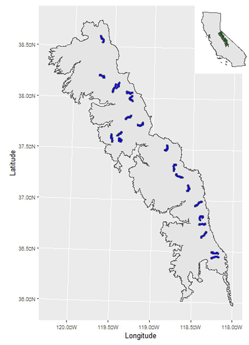
Figure 1. Location of the study region in the Sierra Nevada mountain range of North America. The inset shows the location of the study region (green polygon) in California, United States. The main map shows the geographical extent of the study region, and the blue polygons the locations of 21 randomly selected 10 km² areas where herbaceous biomass samples were collected from 160 randomly located plots distributed among 60 randomly selected meadows >2,500 m.

The study region spanned an elevation range of 2,500–4,000 m along a 350 km north–south gradient (≈ 3° of latitude) and encompassed virtually all of the alpine zone and a large portion of the sub-alpine zone (Figure 1). Transitions from the subalpine to alpine zones are not distinct, but vary with latitude and local topography (Fites-Kaufman et al., 2007). Thus, the existence of a distinct “treeline” between the subalpine and alpine zones is uncommon. Meadows tend to be surrounded by conifer stands in the lower and mid sub-alpine (Lubetkin et al., 2017), while in the upper sub-alpine conifers occur patchily in small, low-statured stands (“krummholz”) scattered among a matrix of rock and meadows. Meadows comprise the main vegetation type in the alpine zone, but they occur patchily and in varying sizes among the dominant rocky features. There can be significant heterogeneity in soil moisture due to fine-scaled variation in topography, which is reflected in considerable within-meadow variation in species composition. Woody plants may be present in meadows (usually willows Salix spp.), but vegetation is overwhelmingly comprised of herbaceous plants.

Analysis overview

We based our analysis on monthly and annual satellite-derived indices of production and productivity. This allowed us to evaluate their temporal and spatial patterns throughout virtually all of the alpine zone and a substantial portion of the upper subalpine zone. The ability to analyze patterns across long temporal and large spatial scales is a clear advantage of satellite indices, but this depends on the accuracy of the indices. Therefore, our initial steps were to: (1) evaluate the accuracy of GIS polygons identified as meadows; and (2) relate data on biomass collected in the field to the satellite index of production (the Normalized Difference Vegetation Index; NDVI). After this, we partitioned the analysis into temporal and spatio-temporal dynamics. Monthly time series were used to investigate temporal dynamics of NDVI and variables derived from annual NDVI time series were used to examine spatio-temporal dynamics. We calculated the proportion of meadows with trends, abrupt changes (changepoints; Beaulieu et al., 2012), neither or both from time series of monthly NDVI. When there was evidence of abrupt changes, we determined the years they occurred. To analyze spatio-temporal dynamics, we derived indices of annual production and productivity, two measures of variability in annual production and productivity, and the overall change in annual production and productivity across years for each meadow. We used geographically weighted regression (GWR) to quantify the spatial distribution of meadows along gradients of latitude, longitude, and elevation for each annual index. We then conducted a distance-decay analysis to evaluate the relationship between similarity among annual temporal indices and distance among meadows. All analyses were conducted in R (R Core Team, 2022).

Data acquisition

Meadow boundaries

We used an Arc GIS shapefile of meadow polygons that was developed by integrating dozens of meadow shapefiles from multiple public and private organizations (Fryjoff-Hung and Viers, 2012). The polygons were for all meadows throughout the SNV, therefore we subset it to include only those ≥2,500 m and within the boundary of our study region. Elevation for each meadow was derived from a 30-m digital elevation model acquired from the US Geological Survey (USGS) National Map.¹

NDVI

Satellite-derived indices have been used for monitoring vegetation biomass and phenology in an extensive range of ecosystems, including those at high elevation (Carlson and Ripley, 1997; Shen et al., 2011). Since the mid-1980’s, NDVI has been perhaps the most widely used of those satellite indices (Pettorelli, 2013). We calculated monthly estimates (January 1985–December 2021) of NDVI from the US Geological Survey Analysis Ready Data archive (ARD; Dwyer et al., 2018). ARD are produced from Landsat 4–9 satellite images that have been accurately georegistered, calibrated, and pre-processed (both top of atmosphere and atmospheric correction). Because ARD are derived from multiple Landsat satellites, there are multiple images for each month (2–7 at 30 m resolution). Therefore, we used the terra package (Hijmans, 2022) in R to derive estimates of monthly maximum NDVI values. NDVI is a ratio between red (R) and near infrared (NIR) wavelengths, but the bands for these wavelengths differ between sensors (i.e., different Landsat satellites). We calculated NDVI as (Band 4 – Band 3)/ (Band 4 + Band 3) for Landsat 4–7 data, and (Band 5 – Band 4) / (Band 5 + Band 4) for Landsat 8 and 9 data. The calculations were done for images where cloud cover was ≤25%.

Because of the high proportion of rock in our study region, we wanted to confirm that NDVI was an accurate index of vegetation biomass. Therefore, we collected herbaceous biomass data that could be directly related to NDVI values. We established 21 randomly selected 10-km² units along a 270 km latitudinal gradient across the study region (Figure 1). The units consisted of 10 km transects with a 1-km buffer (500 m on each side of the transect) separated by a minimum of 5 km. The transects were on trails randomly chosen from a pool of 68 existing routes. Most of the transects traversed the crest of the SNV in a largely east–west orientation and avoided highly traveled routes such as the Pacific Crest Trail.

We randomly selected 60 meadows distributed among the 10-km² regions, then established 1–6 0.25 ha plots (50 m × 50 m) within each meadow (N = 160 plots). Plots within a meadow were separated by a minimum distance of 60 m, with plot centers located approximately in the center of a Landsat pixel. Herbaceous vegetation in four functional groups (forb, grass, rush, sedge) was clipped to ground level in four randomly located 900 cm² quadrats (30 cm × 30 cm) within each plot. The samples for each group were composited within each plot, weighed in the field, then oven dried and weighed in a USGS laboratory on the east side of the SNV (Bishop, California; 37.36° north, 118.40° west). Samples were collected from mid-July to late-August in 2010–2012 and 2014. Biomass (g 3,600 cm²) was calculated as the weight of the composited samples after oven drying.

Analysis

Meadow boundaries

We assessed the accuracy of the meadow polygons with a two-stage ground-truth approach. The first stage consisted of visiting areas identified as meadows within the 21 randomly selected 10-km² regions. We used Arc GIS to calculate centroids for 1 to 9 randomly selected meadow polygons (median = 6) in each 10-km² region (N = 126 total). One of the authors (RK) then used a global positioning unit (GPS) to locate each centroid and classified the surrounding area into one of five landcover classes: meadow, shrub, conifer, mixed conifer-shrub, or rock. Visits to the centroids occurred from 2014 through 2016.

The second stage consisted of visiting an equal number (N = 126) of randomly selected points identified as landcover other than meadows and then classifying the surrounding area into one of the five landcover classes. These points were located in areas outside of but between the 10-km² regions. Visits to these points were made by RK between 2015 and 2019.

Accuracy assessment was made by collapsing the landcover classes into meadow and non-meadow, and then developing a confusion matrix based on the number of correct and incorrect classifications. We then calculated the true positive (sensitivity) and negative (specificity) rates, as well as overall accuracy of the meadow polygon delineations.

NDVI

We used ordinary least-squares regression (OLS) to model the relationship between NDVI and total herbaceous biomass (i.e., summed across the functional groups within each plot i). An exploratory analysis indicated there was a curvilinear relationship between NDVI and biomass (g 3,600 cm²), so we log₁₀-transformed biomass and specified the model as:

$NDV{I}_i~N\left({\mu }_i\mathrm{,}{\sigma }^2\right)$

${\mu }_i=\alpha +{\beta }_1^{\ast }{\log }_{10}{\left(\mathrm{Biomass}\right)}_i+{\epsilon }_{\mathrm{i}}$

with α ~ N(0,σ²), β₁ ~ N(0,σ²), ε_i ~ N(0,σ²).

Temporal dynamics

Because the cloud cover threshold (≤25%) resulted in months with missing data (median = 34 per meadow; range = 12–87), we interpolated and smoothed the raw monthly NDVI values with a state-space model. These are flexible hierarchical time series models where parameter estimation is based on an observation model that is linked to a state (process) model (Auger-Méthé et al., 2021). They have several advantages over other time series models (e.g., ARIMA), including; (1) the partitioning of state and observation variability results in estimates of process variation being less biased by sampling error; (2) the time series do not need to be stationary to estimate the parameters; and (3) missing values are accurately estimated through application of a recursive fitting and smoothing process (the Kalman filter). The structure of a state-space model with seasonality is (Shumway and Stoffer, 2011):

$x_i={\mathrm{B}}_i{x}_{t-1}+u_i+{\mathrm{C}}_i{\mathrm{c}}_t+{\mathrm{w}}_i;\mathrm{the\; state\; process\; with}{\mathrm{w}}_i~\mathrm{MVN}\left(0\mathrm{,}{Q}_i\right)$

$y_i={\mathrm{Z}}_i{x}_t+a_i+{\mathrm{D}}_i{\mathrm{d}}_t+{\mathrm{v}}_i;\mathrm{the\; observation\; process\; with}{\mathrm{v}}_i~\mathrm{MVN}\left(0\mathrm{,}{R}_i\right)$

where x and y are time series values for meadow i at time t, B and Z are parameters for x at time t or in the previous time step t−1, respectively, u and a are rate parameters, C and D are parameters associated with covariates for seasonality c and d, respectively (i.e., month), and w and v are the process and observation errors that are assumed to be multivariate normally (MVN) distributed with a mean of 0 and covariances Q and R, respectively. Because NDVI values are continuous and can be positive or negative, the assumption of MVN was justifiable. We used the imputeTS package (Moritz and Bartz-Beielstein, 2017) to interpolate missing NDVI values and the statespacer package (Beijers, 2022) to conduct the smoothing.

We analyzed temporal dynamics by comparing seven models of monthly NDVI for each meadow. The models included: (1) constant mean (null model: no trend or abrupt shifts in level); (2) 1-month autoregression (random walk); (3) 1-month autoregression and changepoints (random fluctuations between periods of abrupt shifts in level); (4) linear trend (steady increase or decrease over time); (5) 1-month autoregression and linear trend (random walk with drift); (6) linear trend with changepoints (steady increase or decrease between periods of abrupt shifts in level); and (7) 1-month autoregression, linear trend, and changepoints (random fluctuations or steady increase or decrease between periods of abrupt shifts in level). Detection of changepoints (number of changepoints and time, i.e., year) was based on a pruned exact linear time algorithm (PELT; Beaulieu and Killick, 2018). PELT searches for changes in mean and/or variance across sequential time segments using penalized likelihood ratio tests that evaluate where changepoints occur (Killick and Eckley, 2014). PELT assumes that the number of changepoints will increase with time series length, but it will not identify changepoints if the likelihood ratio tests indicate there are none. We specified 3 years as the minimum time segment length and used a modified Bayesian Information Criterion penalty for the likelihood ratio tests (Zhang and Siegmund, 2007; Beaulieu and Killick, 2018). Model comparisons were based on the biased-corrected version of Akaike’s Information Criterion (AICc) and AICc weights (wAICc).

AICc is prone to identifying more complex models as having the most support even though some parameters may have little explanatory power (Ward, 2008). Therefore, we used dynamic linear regression (DLR; Zeileis et al., 2005) to calculate slope parameters for meadows identified by the PELT algorithm as having a trend. The incorporation of autoregressive effects into DLR makes it an appropriate tool for evaluating different types of dynamics, including the existence of linear trends. We used the dynlm package in R (Zeileis, 2019) to specify DLR models with trend and 1- and 12-month autoregression, then calculated the trend coefficients and their 95% confidence interval (CI). Based on the results of the PELT and DLR analyses, we assigned the temporal dynamics of each meadow into one of five classes (Table 1): significant decreasing trend in NDVI, negative but non-significant trend coefficient (the 95% CI of the slope coefficient from the DLR overlapped zero), no trend based on both the PELT and DLR analyses, a positive but non-significant trend (the 95% CI of the slope coefficient from the DLR overlapped zero), and a significant increasing trend in NDVI.

Table 1

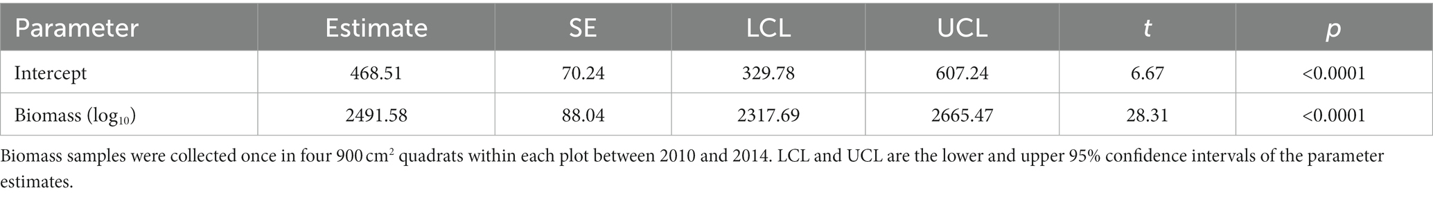
Table 1. The number (N) and percentage of meadows >2,500 m in the Sierra Nevada mountain range of North America where changepoints were detected within five classes of trends between January 1985 and December 2021.

Spatio-temporal dynamics

We used the greenbrown package (Forkel et al., 2013, 2015) to derive an initial set of five indices of annual production and productivity from the monthly time series for each meadow. The indices included: mean growing season NDVI (MGS), peak growing season NDVI (Peak), low growing season NDVI (Trough), the amplitude in growing season NDVI (Amplitude; Peak–Trough), and the rate of spring greenup (RSP). We examined the intra-annual correlations among the indices and removed Peak and Trough because of their high correlations with MGS (mean r = 0.97 and 0.72, respectively), and Amplitude because of its high correlations with RSP (mean r = 0.97). The remaining variables provided indices of annual production (MGS, calculated as the mean NDVI value during the growing season) and productivity (RSP, calculated as the slope in NDVI between the beginning and peak of the growing season). We then calculated three other variables each for MGS and RSP: the coefficient of variation (CV) of temporal variation, the consecutive disparity index (D) of temporal variability, and the overall change in MGS or RSP over the 37-year period (ΔMGS and ΔRSP). The CV is a commonly used measure of temporal variability, but it is not independent of the mean of a time series and is sensitive to uncommon events (Fernández-Martínez et al., 2018). D takes into account the order of values in a time series, is independent of the mean, and not as sensitive to rare events as the CV (Fernández-Martínez et al., 2018). Since D is calculated as the mean rate of change of the log ratios of consecutive values, when D = 1, for example, this indicates that on average variability is ≈ 2.72 × greater than if a time series was constant. Thus, more than simply being an alternative to the CV, D provides additional insight into patterns of temporal variability. ΔMGS and ΔRSP were calculated as the sum of differences between years [e.g., ΔMGS = Σ(MGS_year – MGS_year−1)] and gave a measure of the net increase or decrease of MGS and RSP over the 37 years of the study.

We quantified the distribution of the annual indices along gradients of latitude, longitude and elevation with geographically weighted regression (GWR; Fotheringham et al., 2002). GWR is a variety of least-squares regression that examines how the relationship between dependent and predictor variables varies over space. Whereas traditional (i.e., non-spatial) least-squares would fit a global estimate of the relationship, GWR calculates an estimate for each data point. The non-spatial and spatially varying models can be compared with AICc, and if there is support for the spatial model the local coefficients can be mapped. The core of GWR is the development of a spatial kernel that is a moving window from point to point. The window includes a number of neighboring points determined by the bandwidth, which can be fixed or vary among points (an “adaptive kernel”); narrower bandwidths mean fewer neighboring points are used to calculate the local coefficients. We used the spgwr package (Bivand and Yu, 2020) to calculate the optimal bandwidth for adaptive kernels with a bisquare weighting function, then conducted the GWR for each MGS and RSP variable. We compared GWR and OLS models with wAICc and ANOVA (Fotheringham et al., 2002). We then classified local coefficients as increasing, decreasing or not changing based on the sign of the coefficient and if their 95% CIs overlapped zero.

We reasoned that if meadows with different spatio-temporal dynamics were segregated from each other this would translate to a well-defined distance-decay relationship. Conversely, if there was intermixing of meadows where spatio-temporal dynamics were unlike, then distance-decay relationships would be weak or non-existent. Therefore, we calculated distance matrices from each set of standardized MGS and RSP variables, then regressed those distance matrices against the geographic distances among meadows. We used Euclidean distance because some of the MGS and RSP variables had negative values. The large number of meadows (see Results) made pairwise comparisons of distances computationally unachievable using the full dataset, so we applied a randomization approach to compare slopes of the relationship between observed and permuted geographic distance. This entailed randomly selecting 1,000 meadows in each of 1,000 iterations, then estimating the slope and explained variation (R²) from each iteration. We then calculated the slope based on 1,000 random permutations of the geographic distances within each iteration and compared the mean and 95% CIs of the observed and permuted values. The simba package (Jurasinski and Retzer, 2012) was used to create permutations and calculate slopes from the permuted distances.

Results

The meadow polygons were identified with a very high degree of accuracy. Sensitivity (98%; 123 meadows correctly identified as so) and specificity (97%; 122 points correctly identified as not being meadows) were nearly identical, and overall accuracy was 97.2% (95% CI = 94.4–98.9). A total of 8,149 meadows occurred within the study region. We removed 54 (<1%) from the dataset because sensible NDVI values could not be calculated for them, leaving a working set of 8,095.

There was a very strong relationship between NDVI and total herbaceous biomass (r = 0.914; Table 2 and Figure 2). The relationship was particularly strong in the middle range of biomass values, with a tendency of lower and higher estimates of NDVI than predicted for lower and higher values of biomass, respectively (Figure 2).

Figure 2

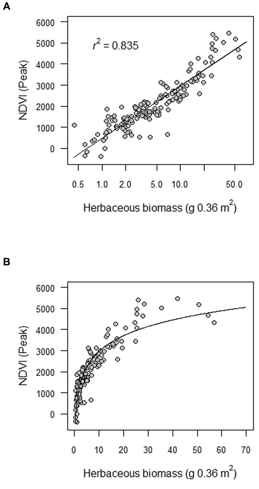
Figure 2. Estimated fit of the relationship between total herbaceous biomass (g per 0.36 m²) and the Normalized Difference Vegetation Index (NDVI) in the Sierra Nevada mountain range of western North America. Biomass samples were collected once in either 2010, 2011, 2012 or 2014 from 160 plots distributed among 60 meadows along a 270 km latitudinal gradient through the upper subalpine and alpine zones. Fitted values were derived from an ordinary least squares regression of log₁₀ transformed biomass values (A); panel (B) shows the curvilinear relationship for untransformed biomass values. NDVI was the peak growing season value associated with a plot in the year the biomass sample was collected.

Table 2

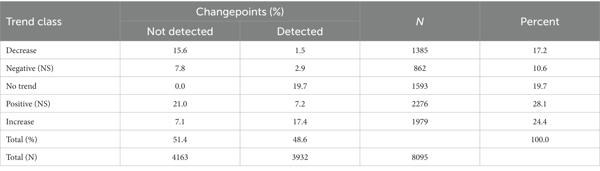
Table 2. Parameter estimates of the relationship between the Normalized Difference Vegetation Index (NDVI) and herbaceous biomass in 160 randomly located plots within 60 randomly selected meadows >2,500 m in the Sierra Nevada mountain range of North America.

Temporal dynamics

Temporal dynamics varied greatly among the meadows (Figure 3). Meadows with strong evidence of a positive trend comprised almost 25% of the total and were 1.5× more common than those with strong evidence of a negative trend (Table 1). Collectively, meadows classified as not having a long-term trend, having a positive but weak trend, or having a positive trend made up >70% of the total. There was marked mixing among the five trend classes when they were plotted along gradients of latitude, longitude, and elevation (Figure 4).

Figure 3

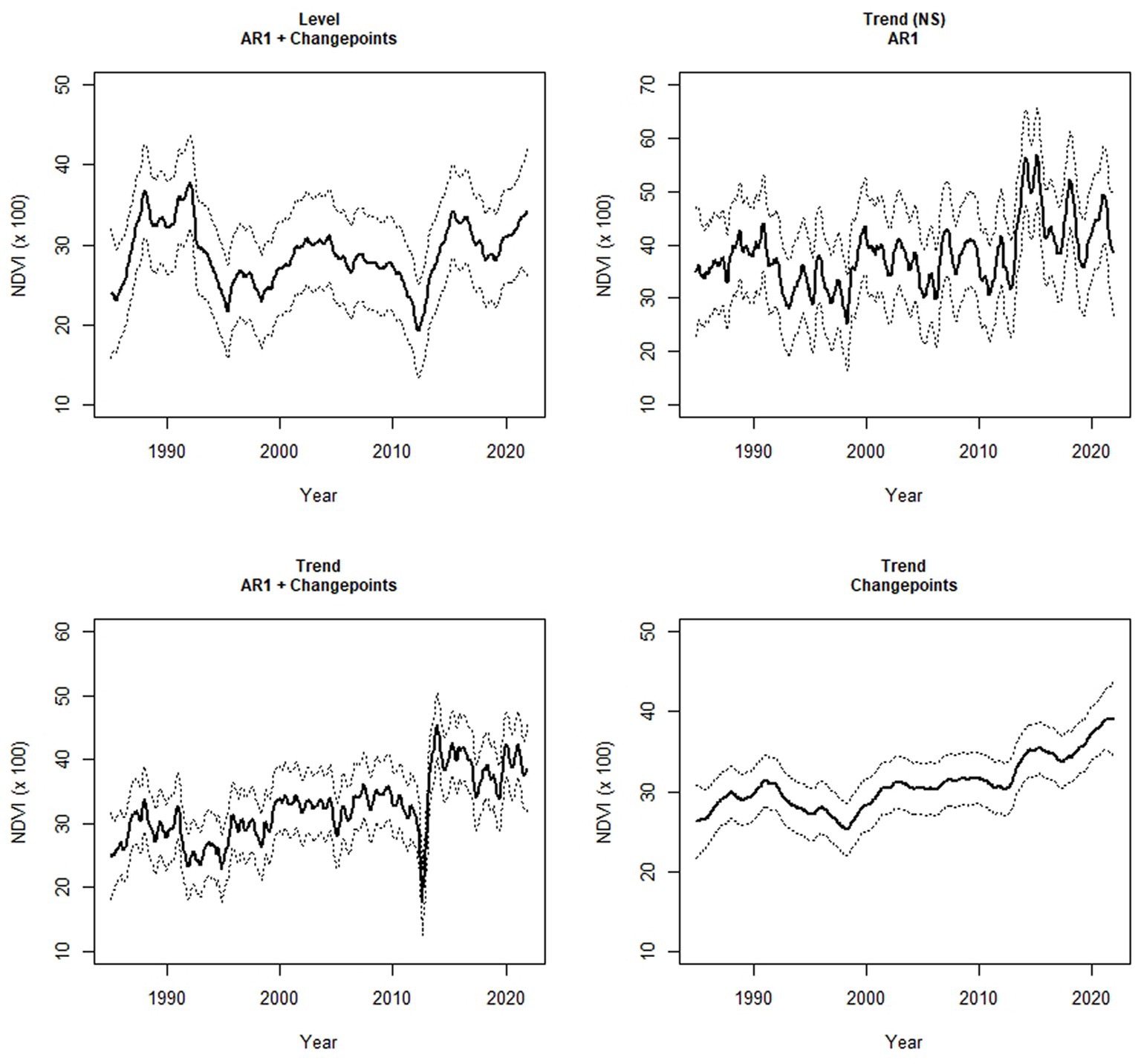
Figure 3. Four randomly selected examples of dynamics in monthly values of the Normalized Difference Vegetation Index (NDVI) from January 1985–December 2021 in meadows in the upper subalpine and alpine zones of the Sierra Nevada mountain range of western North America. The solid line is the smoothed estimate (±95% CI) from a state-space model. NS = a trend was identified as the best model (out of seven) but the 95% CI of the trend coefficient overlapped zero. AR1 = 1-month autoregression.

Figure 4

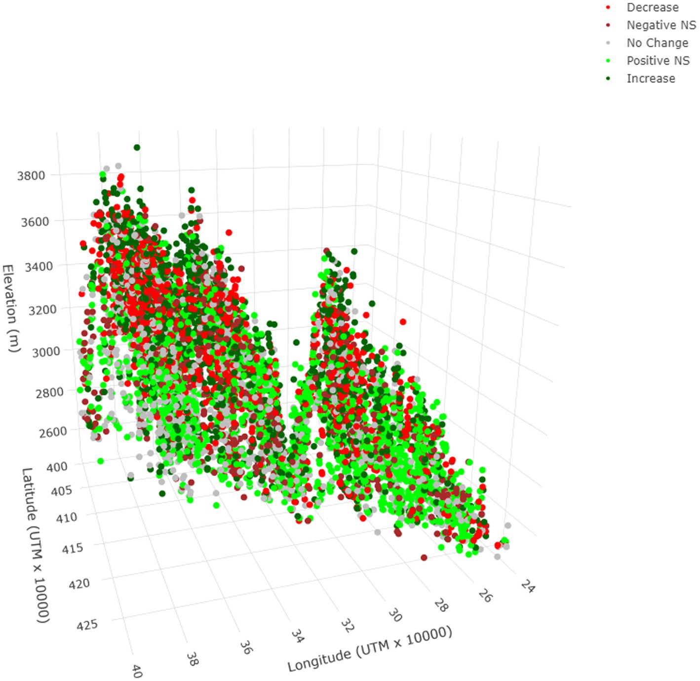
Figure 4. Spatial distribution of meadows in five trend classes in the upper subalpine and alpine zones of the Sierra Nevada mountain range of western North America. Classification of trend was based on smoothed time series of monthly values of the Normalized Difference Vegetation Index (NDVI) from January 1985–December 2021. NS = 95% CI overlapped zero (non-significant).

Changepoints occurred in every year (Figure 5) and were present in the dynamics of >48% of the meadows (N = 3,932). They occurred in 10.4 to 30.5% of the meadows across years, with no indication of a trend of them becoming less or more frequent over time (Figure 5). They also occurred in meadows in all five trend classes, particularly those with no evidence of a trend (100%) or strong evidence of a positive trend (71%) (Table 1).

Figure 5

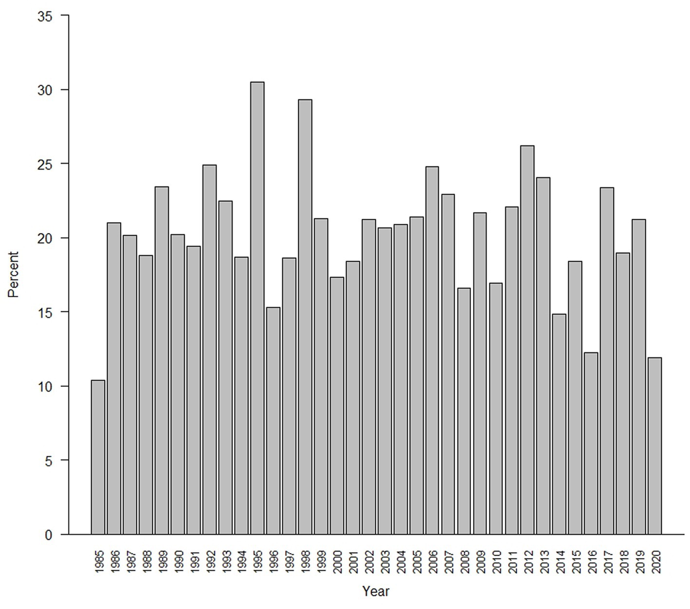
Figure 5. Percentage of meadows in the upper subalpine and alpine zones of the Sierra Nevada mountain range where abrupt changes (changepoints) in the Normalized Difference Vegetation Index (NDVI) were detected.

Spatio-temporal dynamics

There was high heterogeneity in the spatial distribution of the MGS and RSP variables, with wAICc and ANOVA consistently supporting the GWR models for all eight variables (Table 3). The ranges of each of the local coefficients included negative and positive values, and while median values of those ranges were sometimes similar to the values of the global coefficients (MGS, CV of MGS, D for MGS, D for RSP), in other cases they were not (ΔMGS, RSP, CV of RSP; Table 3). Meadows representing the full range of predicted values for the MGS and RSP variables occurred throughout the study region, though there were also clear-cut clusters with similar values (Figures 6A,C, 7A,C, 8A,C, 9A,C).

Table 3

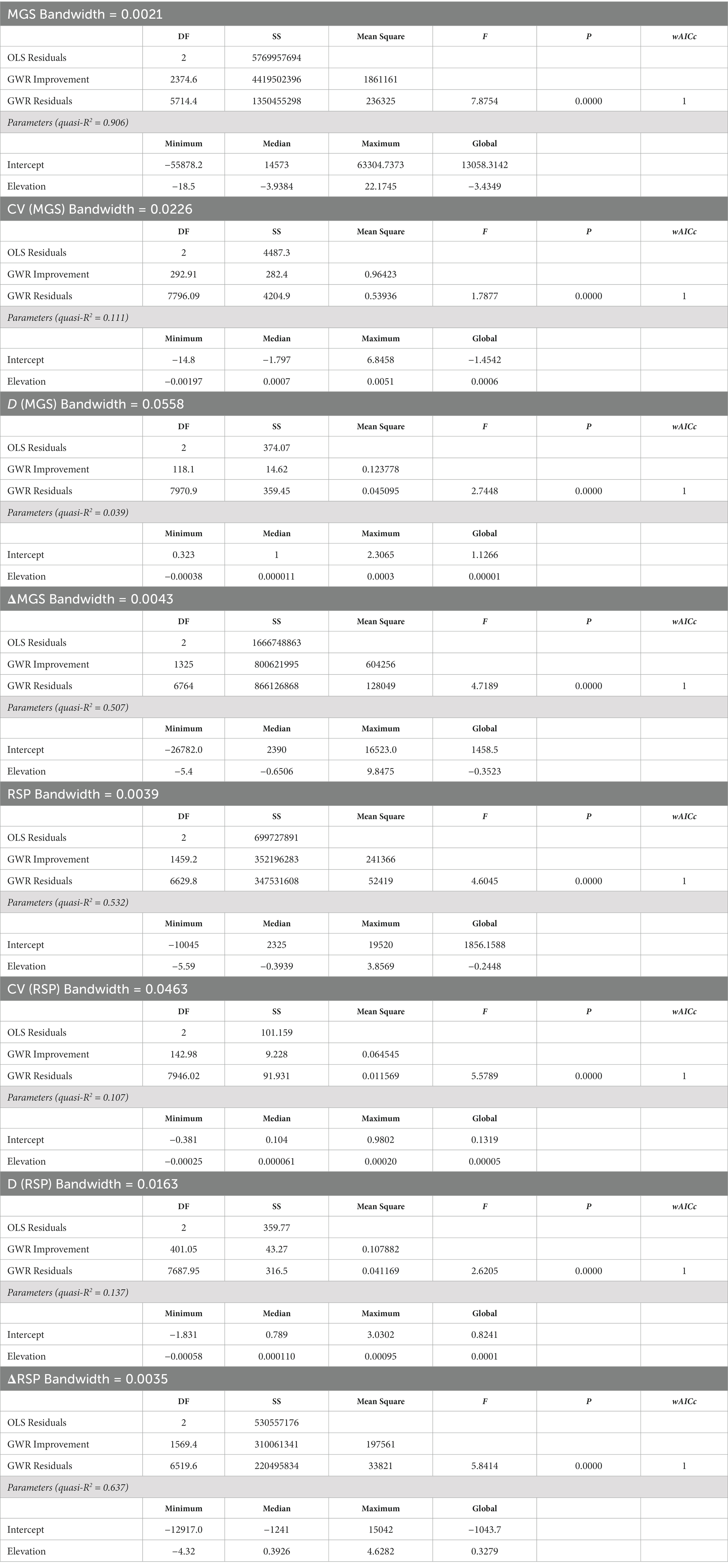
Table 3. Summary statistics for geographically weighted regressions (GWR) of eight indices of annual production (mean growing season value; MGS) and productivity (rate of spring greenup; RSP) in 8,095 meadows >2,500 m in the Sierra Nevada mountain range of North America.

Figure 6

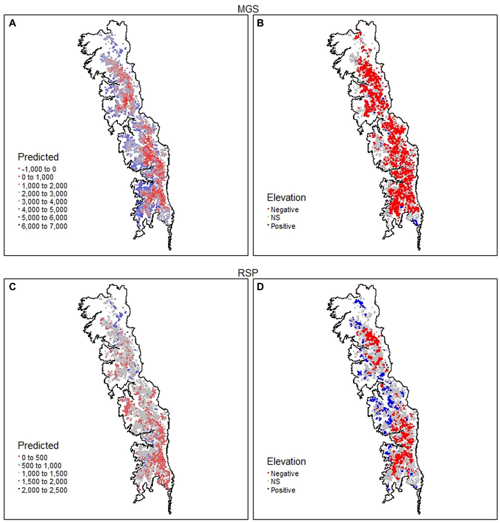
Figure 6. Spatial distribution of mean growing season (MGS) and rate of spring greenup (RSP) values in 8,095 meadows in the upper subalpine and alpine zones of the Sierra Nevada mountain range of western North America. MGS and RSP are annual indices derived from monthly time series (January 1985–December 2021) of the Normalized Difference Vegetation Index (NDVI) for each meadow. Panels (A,C) give predicted values and panels (B,D) direction and significance (p < 0.05) of the relationship with elevation.

Figure 7

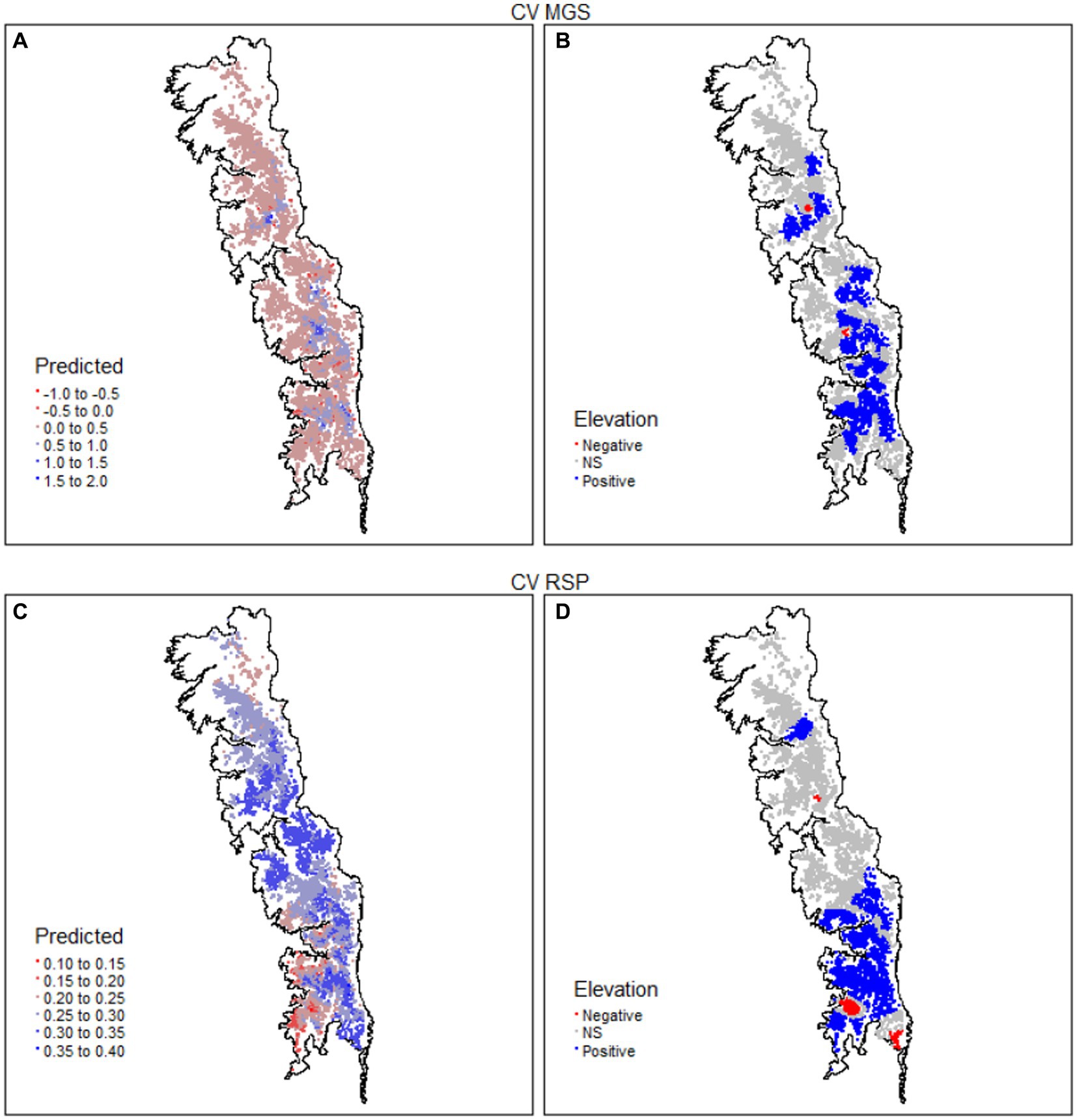
Figure 7. Spatial distribution of the coefficient of variation (CV) for the mean growing season (MGS) and rate of spring greenup (RSP) values of 8,095 meadows in the upper subalpine and alpine zones of the Sierra Nevada mountain range of western North America. MGS and RSP are annual indices derived from time series (January 1985–December 2021) of the Normalized Difference Vegetation Index (NDVI) for each meadow. Panels (A,C) give predicted values and panels (B,D) direction and significance (p < 0.05) of the relationship with elevation.

Figure 8

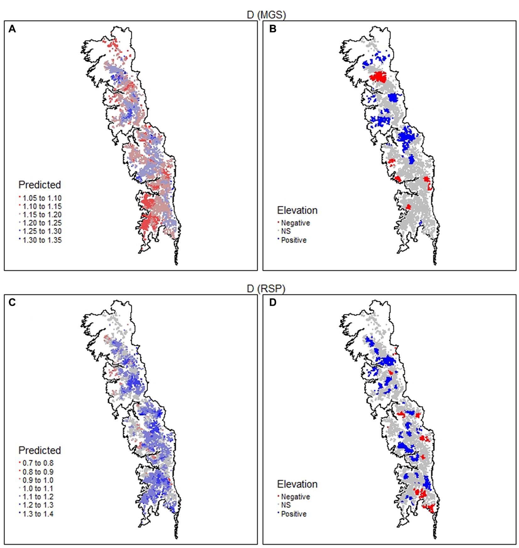
Figure 8. Spatial distribution of the consecutive disparity index (D) for the mean growing season (MGS) and rate of spring greenup (RSP) values of 8,095 meadows in the upper subalpine and alpine zones of the Sierra Nevada mountain range of western North America. MGS and RSP are annual indices derived from time series (January 1985–December 2021) of the Normalized Difference Vegetation Index (NDVI) for each meadow. Panels (A,C) give predicted values and panels (B,D) direction and significance (p < 0.05) of the relationship with elevation.

Figure 9

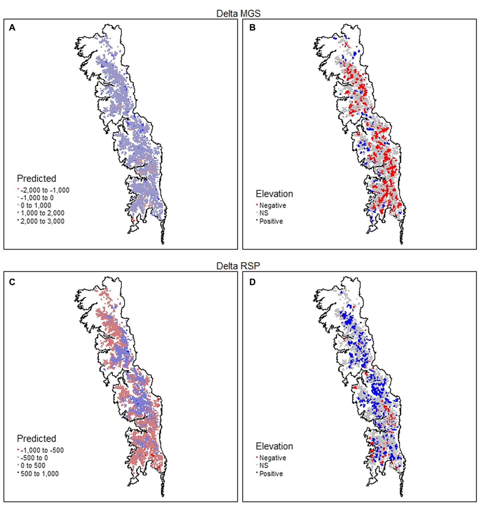
Figure 9. Spatial distribution of the net change (Delta) for mean growing season (MGS) and rate of spring greenup (RSP) values of 8,095 meadows in the upper subalpine and alpine zones of the Sierra Nevada mountain range of western North America. MGS and RSP are annual indices that are derived from time series (January 1985–December 2021) of the Normalized Difference Vegetation Index (NDVI) for each meadow. Panels (A,C) give predicted values and panels (B,D) direction and significance (p < 0.05) of the relationship with elevation.

The GWR model of the relationship between MGS and elevation explained a very high proportion of variation (R² = 0.904; Table 3), with 61.1% of the meadows having significantly negative coefficients (Table 4). Meadows with no indication of a relationship between MGS and elevation comprised 37.6% of the total (Table 4). Overall, meadows with coefficients of varying sign and strength for the relationship between MGS and elevation were intermixed throughout the study region (Figure 6B). The GWR model of the relationship between RSP and elevation explained a moderately high proportion of variation (R² = 0.532; Table 3), but in contrast with MGS the coefficients for 60.2% of the meadows indicated no significant relationship between RSP and elevation. Meadows with significant negative coefficients made up 28.2% of the total (Table 4). The meadows without significant coefficients were distributed throughout the study region, while those with significant negative coefficients were largely absent from the most northerly, southerly, and central areas of the region (Figure 6D). Meadows where there was a significant positive relationship between RSP and elevation made up 11.6% of the total and occurred patchily across the study region (Figure 6D).

Table 4

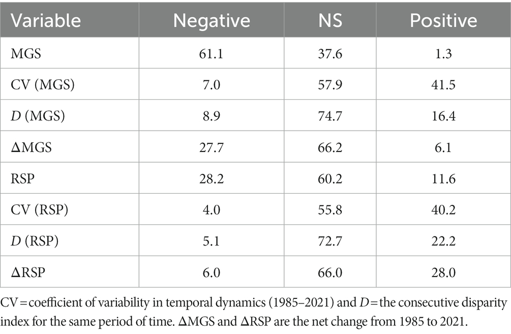
Table 4. The percentage of meadows (N = 8,095) > 2,500 m in the Sierra Nevada mountain range of North America with significantly negative or positive coefficients for eight indices of annual production (mean growing season value; MGS) and productivity (rate of spring greenup; RSP).

The observed CV of MGS was highly skewed (Supplementary Figure S1). Approximately 90% of the values ranged between 0.127 and 0.844 and more than 99% were < 2, but the remainder went as high as 34. The relationship between the CV of MGS and elevation was weak (R² = 0.107; Table 3). Most meadows had no significant relationship with elevation (57.9%; Table 4) and occurred throughout the study region. However, there was notable geographic segregation of meadows with significantly positive coefficients for elevation (41.5%; Table 4 and Figure 7B). These meadows occurred throughout much of the study region but were particularly frequent in the central and southern parts (Figure 7B). The observed CV of RSP was not skewed, though there was one meadow with an extreme value; all other values were < 2 (Supplementary Figure S2). Coefficients in 55.8% of the meadows did not have a significant relationship with elevation, while 40.2% had a significant positive relationship (Tables 3, 4). The spatial distribution of the RSP-elevation relationship was similar to that of the MGS-elevation relationship, though there was a notable lack of positive relationships in the central part of the study region (Figure 7D).

More than 75% of the values for D of MGS > 1 (Supplementary Figure S1). While this was indicative of relatively high inter-annual variability, its relationship with elevation was weak (R² = 0.039; Table 3). Nearly 75% of the meadows had coefficients with no significant relationship with elevation; those with coefficients indicating a significant positive relationship (22.2%) were almost 2× more frequent than those with significant negative coefficients (Table 4). Meadows with non-significant coefficients occurred throughout the study region (Figure 8B). Meadows with significant positive or negative coefficients had markedly different distributions; those with significant positive coefficients were almost entirely absent in the south part of the study region while those with significant negative coefficients were absent in the central part (Figure 8B). The values of D also pointed toward high inter-annual variability in RSP, with more than 70% > 1 (Supplementary Figure S2). Its relationship with elevation was weak (R² = 0.137; Table 3), with almost 73% of the meadows having coefficients indicating no significant relationship. There were more than 4× as many meadows with positive as negative coefficients for D of RSP (Table 4). The ones with positive coefficients occurred patchily throughout the study region, while those with negative coefficients were largely absent in the north (Figure 8D).

GWR R² values for ΔMGS and ΔRSP were 0.507 and 0.637%, respectively. The percentage of meadows with coefficients indicating no significant relationship with elevation was almost identical between ΔMGS and ΔRSP (Table 4). They occurred throughout the study region and were 2.4× to 10× more frequent as meadows with a significant positive or negative relationship (Figures 9B,D and Table 4). Meadows with a significant negative coefficient for ΔMGS (27.7%) occurred patchily throughout the region, as did those with significant positive coefficients for ΔRSP (28%; Figures 9B,D and Table 4). Meadows with significant positive ΔMGS coefficients (6.1%) were distributed sparsely throughout the study region, but those with significant negative ΔRSP coefficients (6%) were largely absent from the north (Figures 9B,D).

There was no indication of a meaningful distance-decay relationship for either the MGS or RSP matrices. Intercepts of the relationship indicated only moderate similarity among meadows even at very short distances, with extremely high variability across the entire range of geographic distances (Supplementary Figures S3, S4). The 95% CI of MGS slope parameters overlapped zero (Figure 10A) and differences between pairwise and permuted slope values were essentially zero (Table 5). The 95% CI of RSP slope parameters was greater than zero (Figure 10B), but the effect size was negligible; differences between pairwise and permuted slope values were essentially zero (Table 5). The mean p-value and R² for the MGS permutations were 0.508 and 0.00087, respectively. Mean p-value and R² for RSP permutations were 0.503 and 0.00469, respectively.

Figure 10

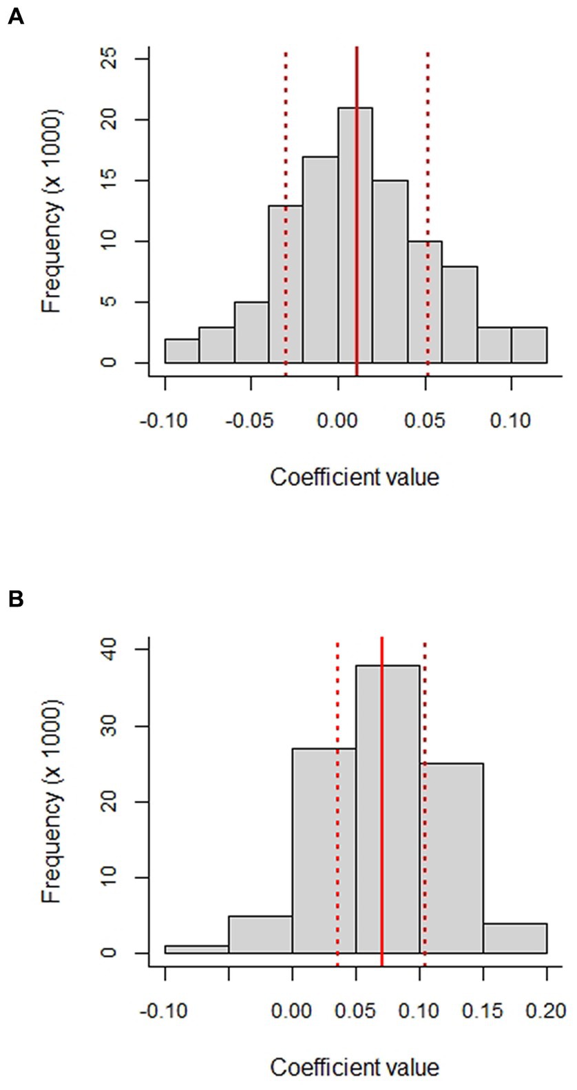
Figure 10. Histograms of slope parameters for the distance-decay relationship between the geographic distance between pairwise combinations of meadows in the upper subalpine and alpine zones of the Sierra Nevada mountain range of western North America and: (A) distance matrices derived from four variables related to the mean annual growing season value (MGS) of the Normalized Difference Vegetation Index (NDVI); and (B) distance matrices derived from four variables related to the rate of spring greenup (RSP). Parameter estimates were estimated from 1,000 random draws (N = 1,000 per draw) from 8,095 meadows. The variables included MGS, the CV of MGS, the consecutive disparity index D of MGS, the net change in MGS from 1985 through 2021 (ΔMGS), RSP, and CV, D, and ΔRSP. Distance matrices were in Euclidean units. See text for further explanation of the variables and how they were derived. The solid red lines are the mean values and the dashed lines the 95% CIs.

Table 5

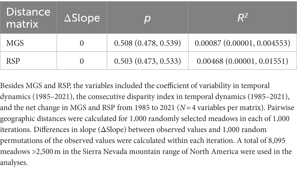
Table 5. Summary statistics from distance-decay analyses based on matrices derived from variables related to annual herbaceous vegetation production (mean growing season value; MGS) and productivity (rate of spring greenup; RSP).

Discussion

We focused the analyses in this study on spatio-temporal patterns so we would have a foundation for developing and testing hypotheses of more mechanistic relationships between environmental heterogeneity and dynamics in meadow condition. Based on the patterns we found, the analyses we conduct in the future will clearly need to focus on temporal variability and spatial heterogeneity more so than general trends. Across four decades and a spatial extent of hundreds of kilometers, we found indices of herbaceous production and productivity in meadows in the subalpine and alpine zones of the SNV pointed strongly toward high levels of variability in both temporal and spatial dynamics. A large portion of the meadows had either no trend or very weak ones, and where trends occurred they often differed in direction. Nearly half of the meadows had a rapid change in production in at least one of the 37 years of the study, but the changes were not associated with trend direction or periods of time with particular conditions (e.g., a series of drought or wet years). Indices of annual production and productivity had weak spatial associations with each other, and indices of net change in production and productivity had almost wholly opposing patterns. Two indices of temporal variability differed somewhat in their spatial pattern, but they were similar in highlighting the intermixing of meadows with different patterns of temporal variability and in having weak relationships with elevation.

NDVI is generally considered to be a useful index of vegetation production (Pettorelli, 2013) and has been used extensively to analyze climate effects on vegetation in high elevation zones of the Tibetan Plateau (Ding et al., 2007; Sun et al., 2013, 2016). It is particularly useful in studies such as ours where the focus is on large scale patterns. We found a strong relationship between herbaceous biomass and NDVI, so have little reason to think our findings could be an artifact of mismatch between plot-based and satellite-based measures of vegetation production. But we also think there are instances where NDVI needs to be used cautiously. In our case we simply wanted to ensure NDVI was an appropriate index of plant biomass in the meadows, so we specified it as being dependent on plant biomass. In other cases though the goal might be to predict herbaceous biomass from NDVI, hence biomass would be dependent on NDVI. In situations where there is a linear relationship between NDVI and biomass the predictions would be straightforward. But in circumstances such as ours where there was an asymptotic relationship between untransformed values, plant biomass would be underestimated at higher values of NDVI. A log transformation would linearize the relationship and put it on a multiplicative scale, but there would need to be an ecological justification, in addition to a statistical rationale, for doing so.

The larger proportion of meadows with increasing than decreasing trends in NDVI suggests warming is having greater positive than negative effects on meadow condition and is consistent with expectations of production increasing because of warmer conditions, a longer growing season, or both (Ganjurjav et al., 2016). However, many meadows had no trend or only a very weak trend. Thus, rather than temporal dynamics indicating a general prevalence of one pattern over others, the most ecologically appropriate interpretation appears to be recognition of a large diversity of patterns, none of which is dominant. The significance of this becomes even greater when spatial intermixing of the temporal dynamics is taken into account. Whether it was for the monthly time series of NDVI or indices of annual production and productivity, the close spatial association of meadows with different dynamics was the most consistent pattern we found. The lack of any meaningful distance-decay pattern was especially effective at showing this; meadows within a few 100 m of each other could have dynamics as dissimilar, or similar, as if they were hundreds of kilometers away. These patterns give a very strong indication of interplay between regionwide, basin, and meadow-scale factors, including climate patterns, snowpack, basin characteristics, topographic complexity, soils, and herbivory.

Intuitively, production and productivity should be greater where temperatures are higher and the growing season longer (Korner, 2003; Shen et al., 2014). The broad occurrence of the negative relationship between elevation and MGS was consistent, at least in part, with the expectation that temperature is setting limits on production. But the extensive distribution of meadows where this relationship was not present shows it is a variable and not completely predictable pattern. The relationship between elevation and RSP was much weaker than that of elevation and MGS, with the spatial distribution of productivity occurring in a patchwork varying greatly in strength and direction along latitudinal, longitudinal and elevation gradients. More so than just the dominance of temperature-related effects, this indicates joint effects of temperature and precipitation likely underlie the variability we observed in meadow production and productivity (Sun and Qin, 2016; Ma et al., 2022). The vast majority of precipitation in the SNV comes as snow, and snowpack is well-recognized to vary at multiple scales throughout the range (Lundquist and Lott, 2007). At a regional scale, differences among winter storm tracks are responsible for the uneven distribution of snow in different parts of the range (Kapnick and Hall, 2010) and likely contributes greatly to not just levels of MGS and RSP, but also the patchy distribution of their variability (CV and D). It is also important to recognize that snow occurs as a regime. Amount (magnitude) and duration are two components of that regime that are particularly relevant to variation in meadow condition in the SNV, but they are not independent and could even have opposite effects on production and productivity (Wang et al., 2017). Meltoff from large snowpacks would generally result in greater moisture availability and higher vegetation production, but larger snowpacks also persist longer. A more extended period of colder temperatures as well as a shortened growing season would be expected to lead to lower productivity, and if growing season length was shortened even further then production would decrease as well. The net effect over large spatial scales of this interplay between amount and duration of snow cover would be an increase in variation along geographic and elevation gradients. Thus, we hypothesize meadows with high production and high rates of productivity in the SNV are most likely to occur in areas where spring meltoff is relatively rapid and snowpacks are intermediate in size and duration.

Physiography and exposure to wind modify snow cover at the basin scale (Loheide et al., 2009; Stephenson et al., 2020; Rittger et al., 2021), which in turn results in variability in water table levels, soil moisture, and thus meadow condition (Lowry et al., 2011; Sun et al., 2016; Wang et al., 2017). Snow cover is more likely to persist longer on shadier slopes and in basins that are relatively protected from winds, resulting in variability along topographic gradients within and across basins. Composition, structure and condition of vegetation within meadows is influenced greatly by hydrology (Weixelman et al., 2011; Viers et al., 2013), and microtopography and soils can exert strong effects on meadow hydrology (Allen-Diaz, 1991). Variation in microtopography is translated primarily to variation in snowpack accumulation while variation in soils primarily affects water table level, but their joint effects can lead to high within-meadow heterogeneity in vegetation condition (McIlroy and Allen-Diaz, 2012; Wang et al., 2017). It is important to note that there is greater likelihood of variation in microtopography and soils with increasing meadow area, therefore we expect within-meadow variation in production to vary greatly along a gradient from smaller to larger meadows.

Herbivory by native and domestic mammals is known to shape vegetation patterns in alpine meadows (Li et al., 2021) and can modify climatic effects on meadow vegetation (Wang et al., 2012; Fu et al., 2015; Niu et al., 2016). A relatively large number of native mammalian herbivores occur in the high elevation zones of the SNV, including larger migratory species (bighorn sheep Ovis canadensis, mule deer Odocoileus hemionus) as well as smaller resident species (marmot Marmota flaviventris, pika Ochotona princeps, ground squirrels Callospermophilus lateralis, Urocitellus beldingii). Meadows are patches of highly nutritious forage for these species and are heavily used by them (Klinger et al., 2015; Stephenson et al., 2020). Widespread overgrazing by domestic sheep (Ovis aries) occurred in the SNV from the mid-19th century to early 20th century, and grazing by cattle was relatively common in some meadows from the mid to latter parts of the 20th century (Ratliff, 1985). In the last several decades, livestock grazing in the SNV has become more carefully managed, though damage to some meadows still occurs (McIlroy and Allen-Diaz, 2012; Roche et al., 2014). Virtually all of the meadows in our study region were on public lands administered by two federal agencies; US National Park Service (NPS) and US Forest Service (FS). Livestock are heavily regulated by NPS, with most grazing occurring intermittently from Equids (horses, mules) at light to moderate stocking levels in a relatively few designated areas (Klinger et al., 2015; Lee et al. 2017). Livestock grazing on FS lands is more extensive than on NPS lands, but it is still relatively light in the high elevation wilderness areas where our meadows occurred. We think it is likely historic and contemporary grazing are influencing at least some of the variability we observed in meadow condition, particularly in localized areas where meadows with opposite trends occurred in close proximity to one another. We also think it is likely that grazing effects are having a greater influence on variability in production and productivity (i.e., CV and D) than on levels of MGS and RSP or the net change in MGS and RSP. In general though, we strongly suspect the heterogeneity in abiotic conditions throughout the range plays a much larger role in structuring the spatial distribution of production and productivity in the SNV than biotic forces.

Outwardly, CV and D gave different impressions of spatial variability in annual production and productivity. The most obvious difference was the large clustering of positive relationships between CV and elevation in the southern and central parts of the SNV, while D had a much patchier distribution of that relationship. It is likely this pattern is an artifact of how the indices measure variability. Because the CV is sensitive to outliers and not independent of the mean, the clustering of positive relationships with elevation is indicative of more extreme values, lower overall values, or both. MGS and RSP decreased with elevation, and elevations are higher and there is more topographic variability in the southern and central parts of the SNV than the north. Therefore, it is not difficult to see why the CV would be greater in these conditions. In contrast, D is independent of the mean and far less sensitive to outliers, and it emphasizes the sequential differences in a series of values. Thus, the spatial distribution of D in the SNV contrasts the areas of high vs. low interannual variability in production and productivity. It is also important to bear in mind that the CV and D both indicated variability in the majority of meadows was not related to elevation. This implies factors other than temperature are responsible for the majority of the variability in production and productivity. These could be relatively localized processes such as heterogeneity in moisture and nutrients (Ren et al., 2010; Ma et al., 2022) or more complex, larger scale interactions between processes such as nitrogen deposition and phenological shifts (Zhang et al., 2015; Fu and Shen, 2017; Wang et al., 2022).

Implications

Temporal dynamics are often characterized by abrupt changes and being dependent on past conditions (“memory”; Beaulieu and Killick, 2018). Consequently, inferences based on dynamics from short-term studies are likely to be misleading, especially in regard to purported “trends.” Ryo et al. (2019) proposed a hierarchical framework that accounts for complexity at different time scales resulting from varying numbers and types of perturbations. Because environmental conditions are highly changeable in most high elevation regions, this concept of scale-dependent variability should be a fundamentally appropriate one to help understand vegetation dynamics in these systems.

Implicitly or explicitly, the interpretation of responses to climate shifts have often been framed from “a big umbrella” perspective, with an emphasis on mean responses and much less on the variability around the mean response. An increasing amount of evidence from both experimental and observational studies indicates variable and complex responses are more likely than broadly consistent ones though, be they at species, community, or ecosystem levels (Klanderud, 2008; Randin et al., 2009; Ma et al., 2022). The diversity and intermixing of spatio-temporal patterns of meadow production and productivity we found is a strong indication “general trends” in meadow condition will be far less meaningful for understanding vegetation dynamics than local patterns resulting from strong heterogeneity in climate and physiognomy. In all likelihood, this will also pertain to montane systems besides the SNV. In conclusion, what is often considered “noise” may often be more informative than a “signal” embedded within a large amount of variability.

Author’s Note

The use of trade, product, or firm names in this publication is for descriptive purposes only and does not imply endorsement by the US Government.

Data availability statement

The satellite data presented in the study are publicly available. The URL for the meadow polygons is https://meadows.ucdavis.edu/meadows/map. The URL for the NDVI data is https://earthexplorer.usgs.gov/.

Author contributions

RK designed the methodology, collected data with the field team, analyzed the data, and led the writing of the manuscript. TS and RK conceived the initial concept. TS provided review and modifications to drafts of the manuscript. JL, LS, and SJ acquired, processed, managed, and conducted preliminary analyses of the satellite data. All authors contributed to reviewing drafts of the manuscript and gave final approval for publication.

Funding

Major funding was provided by the USGS Ecosystems Program, with additional funding from Yosemite National Park and Sequoia and Kings Canyon National Parks.

Acknowledgments

We thank the USGS staff in Bishop, California for collecting the biomass data, especially Jennifer Chase, Ashley Beechan, Anna Godinho, Steven Lee, Lindsay Swinger, Stacey Huskins, Michael Cleaver, Laurel Triatek, Cody Massing, Jon Clark, Bridgett Downs, Drew Maraglia, Carli Morgan, and Brian Hatfield. Steven Lee, Peggy Moore, Sylvia Haultain, Kaitlin Lubetkin, and Jennifer Chase provided a number of important ideas and insights on the dynamics of high elevation meadows.

Conflict of interest

The authors declare that the research was conducted in the absence of any commercial or financial relationships that could be construed as a potential conflict of interest.

Publisher’s note

All claims expressed in this article are solely those of the authors and do not necessarily represent those of their affiliated organizations, or those of the publisher, the editors and the reviewers. Any product that may be evaluated in this article, or claim that may be made by its manufacturer, is not guaranteed or endorsed by the publisher.

Supplementary material

The Supplementary material for this article can be found online at: https://www.frontiersin.org/articles/10.3389/fevo.2023.1184918/full#supplementary-material

SUPPLEMENTARY FIGURE S1 | Distributions related to four indices of annual mean growing season (MGS) values for herbaceous vegetation in 8,095 meadows > 2,500 m in the Sierra Nevada mountain range of North America. CV = coefficient of variability in temporal dynamics (1985–2021) and D = the consecutive disparity index for the same period of time. ΔMGS is the net change from 1985 to 2021. Values were derived from monthly time series of the Normalized Difference Vegetation Index (NDVI) in each meadow.

SUPPLEMENTARY FIGURE S2 | Distributions related to four indices of annual rate of spring greenup (RSP) values for herbaceous vegetation in 8,095 meadows > 2,500 m in the Sierra Nevada mountain range of North America. CV = coefficient of variability in temporal dynamics (1985–2021) and D = the consecutive disparity index for the same period of time. ΔRSP is the net change from 1985 to 2021. Values were derived from monthly time series of the Normalized Difference Vegetation Index (NDVI) in each meadow.

SUPPLEMENTARY FIGURE S3 | Four examples of distance decay relationships for 1,000 randomly selected meadows > 2,500 m in the Sierra Nevada mountain range of North America. The meadows were selected from a total pool of 8,095. Points represent pairwise geographic distances and distances derived from annual herbaceous vegetation production (mean growing season value; MGS), coefficient of variability in temporal dynamics for MGS (1985–2021), the consecutive disparity index in temporal dynamics for MGS (1985–2021), and the net change in MGS from 1985 to 2021. The red horizontal line represents the fitted estimate.

SUPPLEMENTARY FIGURE S4 | Four examples of distance decay relationships for 1,000 randomly selected meadows > 2,500 m in the Sierra Nevada mountain range of North America. The meadows were selected from a total pool of 8,095. Points represent pairwise geographic distances and distances derived from annual herbaceous vegetation productivity (rate of spring greenup; RSP), the coefficient of variability in temporal dynamics for RSP (1985–2021), consecutive disparity index in temporal dynamics for RSP (1985–2021), and net change in RSP from 1985 to 2021. The red horizontal line represents the fitted estimate.

Footnotes

1. ^https://apps.nationalmap.gov/downloader/

References

Allen-Diaz, B. H. (1991). Water table and plant species relationships in Sierra Nevada meadows. Am. Midl. Nat. 126, 30–43. doi: 10.2307/2426147

Crossref Full Text | Google Scholar

Auger-Méthé, M., Newman, K., Cole, D., Empacher, F., Gryba, R., King, A. A., et al. (2021). A guide to state–space modeling of ecological time series. Ecol. Monogr. 91:e01470. doi: 10.1002/ecm.1470

Crossref Full Text | Google Scholar

Beaulieu, C., Chen, J., and Sarmiento, J. L. (2012). Change-point analysis as a tool to detect abrupt climate variations. Philos. Trans. R. Soc. 370, 1228–1249. doi: 10.1098/rsta.2011.0383

Crossref Full Text | Google Scholar

Beaulieu, C., and Killick, R. (2018). Distinguishing trends and shifts from memory in climate data. J. Clim. 31, 9519–9543. doi: 10.1175/JCLI-D-17-0863.1

Crossref Full Text | Google Scholar

Beijers, D. (2022). statespacer: state space modelling in R. R package version 0.4.1.

Google Scholar

Bivand, R, and Yu, D. (2020). spgwr: geographically weighted regression. R package version 0.6-34. Available at: https://CRAN.R-project.org/package=spgwr

Google Scholar

Boelman, N. T., Stieglitz, M., Rueth, H. M., Sommerkorn, M., Griffin, K. L., Shaver, G. R., et al. (2003). Response of NDVI, biomass, and ecosystem gas exchange to long-term warming and fertilization in wet sedge tundra. Oecologia 135, 414–421. doi: 10.1007/s00442-003-1198-3

PubMed Abstract | Crossref Full Text | Google Scholar

Brandt, J. S., Haynes, M. A., Kuemmerle, T., Waller, D. M., and Radeloff, V. C. (2013). Regime shift on the roof of the world: Alpine meadows converting to shrublands in the southern Himalayas. Biol. Conserv. 158, 116–127. doi: 10.1016/j.biocon.2012.07.026

Crossref Full Text | Google Scholar

Carlson, T. N., and Ripley, D. A. (1997). On the relation between NDVI, fractional vegetation cover, and leaf area index. Remote Sens. Environ. 62, 241–252. doi: 10.1016/S0034-4257(97)00104-1

Crossref Full Text | Google Scholar

Cayan, D., Kammerdiener, S., Dettinger, M., Caprio, J., and Peterson, D. (2001). Changes in the onset of spring in the western United States. Bull. Am. Meteorol. Soc. 82, 339–415. doi: 10.1175/1520-0477(2001)082<0399:CITOOS>2.3.CO;2

Crossref Full Text | Google Scholar

Dettinger, M., Alpert, H., Battles, J., Kusel, Jonathan, Safford, Hugh, Fougeres, Dorian, et al., (2018). Sierra Nevada summary report. California’s fourth climate change assessment. Publication No. SUMCCCA4-2018-004. Sacramento, CA: State of California. 94 p

Google Scholar

Ding, M. J., Zhang, Y. L., Liu, L. S., Zhang, W., Wang, Z. F., and Bai, W. Q. (2007). The relationship between NDVI and precipitation on the Tibetan Plateau. J Geogr Sci 17, 259–268. doi: 10.1007/s11442-007-0259-7

Crossref Full Text | Google Scholar

Dirnbock, T., Dullinger, S., and Grabherr, G. (2003). A regional impact assessment of climate and land-use change on alpine vegetation. J. Biogeogr. 30, 401–417. doi: 10.1046/j.1365-2699.2003.00839.x

Crossref Full Text | Google Scholar

Dwyer, J. L., Roy, D. P., Sauer, B., Jenkerson, C. B., Zhang, H. K., and Lymburner, L. (2018). Analysis ready data: enabling analysis of the landsat archive. Remote Sens. 10:1363. doi: 10.3390/rs10091363

Crossref Full Text | Google Scholar

Epanchin, P. N., Knapp, R. A., and Lawler, S. P. (2010). Nonnative trout impact an alpine-nesting bird by altering aquatic-insect subsidies. Ecology 91, 2406–2415. doi: 10.1890/09-1974.1

PubMed Abstract | Crossref Full Text | Google Scholar

Felde, V. A., Kapfer, J., and Grytnes, J.-A. (2012). Upward shift in elevational plant species ranges in Sikkilsdalen, Central Norway. Ecography 35, 922–932. doi: 10.1111/j.1600-0587.2011.07057.x

Crossref Full Text | Google Scholar

Fernández-Martínez, M., Vicca, S., Janssens, I. A., Carnicer, J., Martın-Vide, J., and Penuelas, J. (2018). The consecutive disparity index, D: a measure of temporal variability in ecological studies. Ecosphere 9:e02527. doi: 10.1002/ecs2.2527

Crossref Full Text | Google Scholar

Fites-Kaufman, J. A., Runel, P., Stephenson, N. L., and Weixelman, D. A. (2007). “Montane and subalpine vegetation of the Sierra Nevada and Cascade ranges” in Terrestrial vegetation of California. eds. M. G. Barbour, T. Keeler-Wolf, and A. A. Schoenherr (University of California Press), 456–501.

Google Scholar

Forkel, M., Carvalhais, N., Verbesselt, J., Mahecha, M. D., Neigh, C., and Reichstein, M. (2013). Trend change detection in NDVI time series: effects of inter-annual variability and methodology. Remote Sens. 5, 2113–2144. doi: 10.3390/rs5052113

Crossref Full Text | Google Scholar

Forkel, M., Migliavacca, M., Thonicke, K., Reichstein, M., Schaphoff, S., Weber, U., et al. (2015). Co-dominant water control on global inter-annual variability and trends in land surface phenology and greenness. Glob. Chang. Biol. 21, 3414–3435. doi: 10.1111/gcb.12950

PubMed Abstract | Crossref Full Text | Google Scholar

Fotheringham, A.S., Brunsdon, C., and Charlton, M. (2002). Geographically weighted regression: The analysis of spatially varying relationships. Chichester: Wiley.

Google Scholar

Fryjoff-Hung, A., and Viers, J.H. (2012). Sierra Nevada multi-source meadow polygons compilation (v 1.0), Center for Watershed Sciences, UC Davis. December 2012. Available at: http://meadows.ucdavis.edu/

Google Scholar

Fu, G., and Shen, Z.-X. (2017). Response of alpine soils to nitrogen addition on the Tibetan Plateau: a meta-analysis. Appl. Soil Ecol. 114, 99–104. doi: 10.1016/j.apsoil.2017.03.008

Crossref Full Text | Google Scholar

Fu, G., Sun, W., Yu, C. Q., Zhang, X.-Z., Shen, Z.-X., Li, Y. L., et al. (2015). Clipping alters the response of biomass production to experimental warming: a case study in an alpine meadow on the Tibetan Plateau, China. J. Mt. Sci. 12, 935–942. doi: 10.1007/s11629-014-3035-z

Crossref Full Text | Google Scholar

Fu, G., Zhang, X., Zhang, Y., Shi, P., Li, Y., Zhou, Y., et al. (2013). Experimental warming does not enhance gross primary production and above-ground biomass in the alpine meadow of Tibet. J. Appl. Remote. Sens. 7:073505. doi: 10.1117/1111.jrs.1117.073505

Crossref Full Text | Google Scholar

Ganjurjav, H., Gaoa, Q., Gornish, E. S., Schwartz, M. W., Lianga, Y., Cao, X., et al. (2016). Differential response of alpine steppe and alpine meadow to climate warming in the Central Qinghai–Tibetan Plateau. Agric. For. Meteorol. 223, 233–240. doi: 10.1016/j.agrformet.2016.03.017

Crossref Full Text | Google Scholar

Haugo, R. D., Halpern, C. B., and Bakker, J. D. (2011). Landscape context and long-term tree influences shape the dynamics of forest-meadow ecotones in mountain ecosystems. Ecosphere 2:art91. doi: 10.1890/ES11-00110.1

Crossref Full Text | Google Scholar

Hayhoe, K., Cayan, D., Field, C. B., Frumhoff, P. C., Maurer, E. P., Miller, N. L., et al. (2004). Emissions pathways, climate change, and impacts on California. Proc. Natl. Acad. Sci. U. S. A. 101, 12422–12427. doi: 10.1073/pnas.0404500101

Crossref Full Text | Google Scholar

Hijmans, R. J. (2022). terra: Spatial Data Analysis. R package version 1.5-21. Available at: https://CRAN.R-project.org/package=terra

Google Scholar

Hik, D. S., McColl, C. J., and Boonstra, R. (2001). Why are Arctic ground squirrels more stressed in the boreal forest than in alpine meadows? Ecoscience 8, 275–288. doi: 10.1080/11956860.2001.11682654

Crossref Full Text | Google Scholar

Hillebrand, H., Donohue, I., Harpole, W. S., Hodapp, D., Kucera, M, Lewandowska, A. M., et al. (2020). Thresholds for ecological responses to global change do not emerge from empirical data. Nat. Ecol. Evol 4, 1502–1509. doi: 10.1038/s41559-020-1256-9

Crossref Full Text | Google Scholar

Huelber, K., Gottfried, M., Pauli, H., Reiter, K., Winkler, M., and Grabherr, G. (2006). Phenological responses of snowbed species to snow removal dates in the Central Alps: implications for climate warming. Arctic Antarctic Alpine Res. 38, 99–103. doi: 10.1657/1523-0430(2006)038[0099:PROSST]2.0.CO;2

Crossref Full Text | Google Scholar

Inouye, D. W. (2008). Effects of climate change on phenology, frost damage, and floral abundance of montane wildflowers. Ecology 89, 353–362. doi: 10.1890/06-2128.1

Crossref Full Text | Google Scholar

Jurasinski, G., and Kreyling, J. (2007). Upward shift of alpine plants increases floristic similarity of mountain summits. J. Veg. Sci. 18, 711–718. doi: 10.1111/j.1654-1103.2007.tb02585.x

Crossref Full Text | Google Scholar

Jurasinski, G., and Retzer, V. (2012). simba: a collection of functions for similarity analysis of vegetation data. R package version 0.3-5. Available at: https://CRAN.R-project.org/package=simba

Google Scholar

Kapnick, S., and Hall, A. (2010). Observed climate–snowpack relationships in California and their implications for the future. J. Clim. 23, 3446–3456. doi: 10.1175/2010JCLI2903.1

Crossref Full Text | Google Scholar

Killick, R., and Eckley, I. A. (2014). changepoint: an R package for changepoint analysis. J. Stat. Softw. 58, 1, –19. doi: 10.18637/jss.v058.i03

Crossref Full Text | Google Scholar

Klanderud, K. (2008). Species-specific responses of an alpine plant community under simulated environmental change. J. Veg. Sci. 19, 363–372. doi: 10.3170/2008-8-18376

Crossref Full Text | Google Scholar

Klinger, R.C., Few, A.P., Knox, K.A., Hatfield, B.E., Clark, J., German, D.W., et al., (2015). Evaluating potential overlap between pack stock and Sierra Nevada bighorn sheep (Ovis canadensis sierrae) in Sequoia and Kings Canyon National Parks, California : Reston, VA: U.S. Geological Survey Open-File Report 2015-1102, 46.

Google Scholar

Korner, C. (2003). Alpine plant life: functional plant ecology of high mountain ecosystems. 2nd. Springer, Berlin, Germany.

Google Scholar

Krajik, K. (2004). All downhill from here? Science 303, 1600–1602. doi: 10.1126/science.303.5664.1600

Crossref Full Text | Google Scholar

Kudo, G., Kimura, M., Kasagi, T., Kawai, Y., and Hirai, A. S. (2010). Habitat specific responses of alpine plants to climatic amelioration: comparison of fellfield to snowbed communities. Arctic Antarctic Alpine Res 42, 438–448. doi: 10.1657/1938-4246-42.4.438

Crossref Full Text | Google Scholar

Lamy, T., Wisnoski, N. I., Andrade, R., Castorani, M. C. N., Compagnoni, A., Lany, N., et al. (2021). The dual nature of metacommunity variability. Oikos 130, 2078–2092. doi: 10.1111/oik.08517

Crossref Full Text | Google Scholar

Lee, S. R., Berlow, E. L., Ostoja, S. M., Brooks, M. L., Genin, A., and Matchett, J. R. (2017). A multi-scale evaluation of pack stock effects on subalpine meadow plant communities in the Sierra Nevada. PLoS ONE 12:e0178536. doi: 10.1371/journal.pone.0178536

PubMed Abstract | Crossref Full Text | Google Scholar

Lenoir, J., Gegout, J. C., Marquet, P. A., de Ruffray, P., and Brisse, H. (2008). A significant upward shift in plant species optimum elevation during the 20th century. Science 320, 1768–1771. doi: 10.1126/science.1156831

PubMed Abstract | Crossref Full Text | Google Scholar

Li, J., Qi, H. H., Duan, Y. Y., and Guo, Z. G. (2021). Effects of plateau pika disturbance on the spatial heterogeneity of vegetation in alpine meadows. Front. Plant Sci. 12:771058. doi: 10.3389/fpls.2021.771058

PubMed Abstract | Crossref Full Text | Google Scholar

Loheide, S. P., Deitchman, R. S., Cooper, D. J., Wolf, E. C., Hammersmark, C. T., and Lundquist, J. D. (2009). A framework for understanding the hydroecology of impacted wet meadows in the Sierra Nevada and Cascade Ranges, California, USA. Hydrogeol. J. 17, 229–246. doi: 10.1007/s10040-008-0380-4

Crossref Full Text | Google Scholar

Loheide, S. P., and Gorelick, S. M. (2007). Riparian hydroecology: a coupled model of the observed interactions between groundwater flow and meadow vegetation patterning. Water Resour. Res. 43:W07414. doi: 10.1029/2006WR005233

Crossref Full Text | Google Scholar

Lowry, C. S., Loheide, S. P., Moore, C. E., and Lundquist, J. D. (2011). Groundwater controls on vegetation composition and patterning in mountain meadows. Water Resour. Res. 47:W00J11. doi: 10.1029/2010WR010086

Crossref Full Text | Google Scholar

Lubetkin, K. C., Westerling, A. L., and Kueppers, L. M. (2017). Climate and landscape drive the pace and pattern of conifer encroachment into subalpine meadows. Ecol. Appl. 27, 1876–1887. doi: 10.1002/eap.1574

PubMed Abstract | Crossref Full Text | Google Scholar

Lundquist, J. D., and Lott, F. (2007). Using inexpensive temperature sensors to monitor the duration and heterogeneity of snow-covered areas. Water Resour. Res. 44. doi: 10.1029/2008WR007035

Crossref Full Text | Google Scholar

Ma, Y., Tian, L., Qu, G., Li, R., Wang, W., and Zhao, J. (2022). Precipitation alters the effects of temperature on the ecosystem multifunctionality in alpine meadows. Front. Plant Sci. 12:824296. doi: 10.3389/fpls.2021.824296

Crossref Full Text | Google Scholar

Malanson, G. P., and Fagre, D. B. (2013). Spatial contexts for temporal variability in alpine vegetation under ongoing climate change. Plant Ecol. 214, 1309–1319. doi: 10.1007/s11258-013-0253-3

Crossref Full Text | Google Scholar

McIlroy, S. K., and Allen-Diaz, B. H. (2012). Plant community distribution along water table and grazing gradients in montane meadows of the Sierra Nevada Range (California, USA). Wetlands Ecol. Manag. 20, 287–296. doi: 10.1007/s11273-012-9253-7

Crossref Full Text | Google Scholar

Moritz, S., and Bartz-Beielstein, T. (2017). imputeTS: time series missing value imputation in R. R J. 9, 207–218. doi: 10.32614/RJ-2017-009

Crossref Full Text | Google Scholar

Mote, P. W., Clark, M., and Hamlet, A. F. (2004). Variability and trends in mountain snowpack in western North America. Preprints, 15th Symp. on global change and climate variations, Seattle, WA, Amer. Meteor. Soc. Vol. 5.

Google Scholar

Mote, P., Hamlet, A., Clark, M., and Lettenmaier, D. (2005). Declining mountain snowpack in western North America. Bull. Am. Meteorol. Soc. 86, 39–49. doi: 10.1175/BAMS-86-1-39

Crossref Full Text | Google Scholar

Niu, K., He, J. S., and Lechowicz, M. J. (2016). Grazing-induced shifts in community functional composition and soil nutrient availability in Tibetan alpine meadows. J. Appl. Ecol. 53, 1554–1564. doi: 10.1111/1365-2664.12727

Crossref Full Text | Google Scholar

Packer, J. G. (1974). Differentiation and dispersal in alpine floras. Arctic Alpine Res. 6, 117–128. doi: 10.1080/00040851.1974.12003768

Crossref Full Text | Google Scholar

Parmesan, C., and Yohe, G. (2003). A globally coherent fingerprint of climate change impacts across natural systems. Nature 421, 37–42. doi: 10.1038/nature01286

Crossref Full Text | Google Scholar

Patton, D. R., and Judd, B. I. (1970). Role of wet meadows as wildlife habitat in southwest. J. Range Manag. 23, 272–276. doi: 10.2307/3896220

Crossref Full Text | Google Scholar

Pauli, H., Gottfried, M., Dullinger, S., Abdaladze, O., Akhalkatsi, M., Alonso, J. L. B., et al. (2012). Recent plant diversity changes on Europe’s mountain summits. Science 336, 353–355. doi: 10.1126/science.1219033

PubMed Abstract | Crossref Full Text | Google Scholar

Pauli, H., Gottfried, M., Reiter, K., Klettner, C., and Grabherr, G. (2007). Signals of range expansions and contractions of vascular plants in the high Alps: observations (1994-2004) at the GLORIA master site Schrankogel, Tyrol, Austria. Glob. Chang. Biol. 13, 147–156. doi: 10.1111/j.1365-2486.2006.01282.x

Crossref Full Text | Google Scholar

Pettorelli, N. (2013). The normalized difference vegetation index. New York: Oxford University Press. 224.

Google Scholar

R Core Team (2022). R: A language and environment for statistical computing. R Foundation for Statistical Computing, Vienna, Austria.

Google Scholar

Randin, C. F., Engler, R., Normand, S., Zappa, M., Zimmermann, N. E., Pearman, P. B., et al. (2009). Climate change and plant distribution: local models predict high-elevation persistence. Glob. Chang. Biol. 15, 1557–1569. doi: 10.1111/j.1365-2486.2008.01766.x

Crossref Full Text | Google Scholar

Ratliff, R.D. (1985). Meadows in the Sierra Nevada of California: state of knowledge. Gen. Tech. Rep. PSW-GTR-84. Berkeley, CA: U.S. Department of Agriculture, Forest Service, Pacific Southwest Forest and Range Experiment Station. 52 p.

Google Scholar

Ren, Z., Li, Q., Chu, C., Zhao, L., Zhang, J., Ai, D., et al. (2010). Effects of resource additions on species richness and ANPP in an alpine meadow community. J. Plant Ecol. 3, 25–31. doi: 10.1093/jpe/rtp034

Crossref Full Text | Google Scholar

Ren, Y., Yang, K., Wang, H., Zhao, L., Chen, Y., Zhou, X., et al. (2021). The South Asia monsoon break promotes grass growth on the Tibetan plateau. J. Geophys. Res. 126:e2020JG005951. doi: 10.1029/2020JG005951

Crossref Full Text | Google Scholar

Rittger, K., Krock, M., Kleiber, W., Bair, E. H., Brodzik, M. J., Stephenson, T. R., et al. (2021). Multi-sensor fusion using random forests for daily fractional snow cover at 30 m. Remote Sens. Environ. 264:112608. doi: 10.1016/j.rse.2021.112608

Crossref Full Text | Google Scholar

Roche, L. M., O’Geen, A. T., Latimer, A. M., and Eastburn, D. J. (2014). Montane meadow hydropedology, plant community, and herbivore dynamics. Ecosphere 5:art150. doi: 10.1890/ES14-00173.1

Crossref Full Text | Google Scholar

Ryo, M., Aguilar-Trigueros, C. A., Pinek, L., Muller, L. A. H., and Rillig, M. C. (2019). Basic principles of temporal dynamics. Trends Ecol. Evol. 34, 723–733. doi: 10.1016/j.tree.2019.03.007

Crossref Full Text | Google Scholar

Scherrer, D., and Körner, C. (2011). Topographically controlled thermal-habitat differentiation buffers alpine plant diversity against climate warming. J. Biogeogr. 38, 406–416. doi: 10.1111/j.1365-2699.2010.02407.x

Crossref Full Text | Google Scholar

Shen, Z., Fu, G., Yu, C., Sun, W., and Zhang, X. (2014). Relationship between the growing season maximum enhanced vegetation index and climatic factors on the Tibetan plateau. Remote Sens. 6, 6765–6789. doi: 10.3390/rs6086765

Crossref Full Text | Google Scholar

Shen, M. G., Tang, Y. H., Chen, J., Zhu, X. L., and Zheng, Y. H. (2011). Influences of temperature and precipitation before the growing season on spring phenology in grasslands of the central and eastern Qinghai-Tibetan Plateau. Agric. For. Meteorol. 151, 1711–1722. doi: 10.1016/j.agrformet.2011.07.003

Crossref Full Text | Google Scholar

Shumway, R.H., and Stoffer, D.S. (2011). Time series analysis and its applications: with R examples. Springer: New York, USA.

Google Scholar

Song, M. H., Hu, Q., Tian, Y., and Ouyang, H. (2012). Seasonal patterns of root and shoot interactions in an alpine meadow on the Tibetan Plateau. J. Plant Ecol. 5, 182–190. doi: 10.1093/jpe/rtq032

Crossref Full Text | Google Scholar

Song, M. H., Tian, Y. Q., and Xu, X. L. (2006). Interactions between root and shoot competition among four plant species in an alpine meadow on the Tibetan Plateau. Acta Oecol. 29, 214–220. doi: 10.1016/j.actao.2005.10.005

Crossref Full Text | Google Scholar

Stephenson, T. R., German, D. W., Cassirer, E. F., Walsh, D. P., Blum, M. E., Cox, M., et al. (2020). Linking population performance to nutritional condition in an alpine ungulate. J. Mammal. 101, 1244–1256. doi: 10.1093/jmammal/gyaa091

PubMed Abstract | Crossref Full Text | Google Scholar

Stewart, I. T. (2009). Changes in snowpack and snowmelt runoff for key mountain regions. Hydrol. Process. 23, 78–94. doi: 10.1002/hyp.7128

Crossref Full Text | Google Scholar

Storer, T.I., Usinger, R.L., and Lukas, D. (2004). Sierra Nevada natural history. Berkeley: University of California Press. p. 592

Google Scholar

Sun, J., Cheng, G. W., Li, W. P., Sha, Y. K., and Yang, Y. C. (2013). On the variation of NDVI with the principal climatic elements in the Tibetan Plateau. Remote Sens. 5, 1894–1911. doi: 10.3390/rs5041894

Crossref Full Text | Google Scholar

Sun, J., and Qin, X. (2016). Precipitation and temperature regulate the seasonal changes of NDVI across the Tibetan plateau. Environ. Earth Sci. 75:291. doi: 10.1007/s12665-015-5177-x

Crossref Full Text | Google Scholar

Sun, J., Qin, X., and Yang, J. (2016). The response of vegetation dynamics of the different alpine grassland types to temperature and precipitation on the Tibetan Plateau. Environ. Monit. Assess. 188:20. doi: 10.1007/s10661-015-5014-4

PubMed Abstract | Crossref Full Text | Google Scholar

Testolin, R., Attorre, F., and Jiménez-Alfaro, B. (2020). Global distribution and bioclimatic characterization of alpine biomes. Ecography 43, 779–788. doi: 10.1111/ecog.05012

Crossref Full Text | Google Scholar

Thorne, J. H., Dobrowski, S., and Safford, H. D. (2007). A 70-year review of landscape change across the Sierra Nevada Ecological Society of America Annual Meeting Abstracts.

Google Scholar

Verrall, B., and Pickering, C. M. (2020). Alpine vegetation in the context of climate change: a global review of past research and future directions. Sci. Total Environ. 748:141344. doi: 10.1016/j.scitotenv.2020.141344

PubMed Abstract | Crossref Full Text | Google Scholar

Viers, J.H., Purdy, S.E., Peek, R.A., Fryjoff-Hung, A., Santos, N.R., Katz, J.V.E., et al., (2013). Montane meadows in the Sierra Nevada: changing hydroclimatic conditions and concepts for vulnerability assessment. Center for Watershed Sciences Technical Report (CWS-2013-01), University of California, Davis, Davis. pp. 63.

Google Scholar

Walther, G. R., Beissner, S., and Burga, C. A. (2005). Trends in the upward shift of alpine plants. J. Veg. Sci. 16, 541–548. doi: 10.1111/j.1654-1103.2005.tb02394.x

Crossref Full Text | Google Scholar

Wang, S. P., Duan, J. C., Xu, G. P., Wang, Y. F., Zhang, Z.-H., Rui, Y. C., et al. (2012). Effects of warming and grazing on soil N availability, species composition, and ANPP in an alpine meadow. Ecology 93, 2365–2376. doi: 10.1890/11-1408.1

PubMed Abstract | Crossref Full Text | Google Scholar

Wang, J., Li, M., Yu, C., and Fu, G. (2022). The change in environmental variables linked to climate change has a stronger effect on aboveground net primary productivity than does phenological change in alpine grasslands. Front. Plant Sci. 12:798633. doi: 10.3389/fpls.2021.798633

PubMed Abstract | Crossref Full Text | Google Scholar

Wang, S., Wang, X., Chen, G., Yang, Q., Wang, B., Ma, Y., et al. (2017). Complex responses of spring alpine vegetation phenology to snow cover dynamics over the Tibetan Plateau, China. Sci. Total Environ. 593-594, 449–461. doi: 10.1016/j.scitotenv.2017.03.187

Crossref Full Text | Google Scholar

Ward, E. J. (2008). A review and comparison of four commonly used Bayesian and maximum likelihood model selection tools. Ecol. Model. 211, 1–10. doi: 10.1016/j.ecolmodel.2007.10.030

Crossref Full Text | Google Scholar

Weixelman, D.A., Hill, B.A., Cooper, D.J., Berlow, E.L., Viers, J.H., Purdy, S.E., et al., (2011). A field key to meadow Hydrogeomorphic types for the Sierra Nevada and southern Cascade ranges in California. Tech. Rep. R5-TP-034. U.S. Department of Agriculture, Forest Service, Pacific Southwest Region Gen Vallejo, California, p. 34.

Google Scholar

Xiao, J., Dong, S., Shen, H., Li, S., Wessell, K., Liu, S., et al. (2022). N addition overwhelmed the effects of P addition on the soil C, N, and P cycling genes in alpine meadow of the Qinghai-Tibetan Plateau. Front. Plant Sci. 13:860590. doi: 10.3389/fpls.2022.860590

PubMed Abstract | Crossref Full Text | Google Scholar

Zeileis, A. (2019). dynlm: dynamic linear regression. R package version 0.3-6. Available at: https://CRAN.R-project.org/package=dynlm

Google Scholar

Zeileis, A., Leisch, F., Kleiber, C., and Hornik, K. (2005). Monitoring structural change in dynamic econometric model. J. Appl. Econ. 20, 99–121. doi: 10.1002/jae.776

Crossref Full Text | Google Scholar

Zhang, N. R., and Siegmund, D. O. (2007). A modified Bayes information criterion with applications to the analysis of comparative genomic hybridization data. Biometrics 63, 22–32. doi: 10.1111/j.1541-0420.2006.00662.x

Crossref Full Text | Google Scholar

Zhang, X.-Z., Shen, Z.-X., and Fu, G. (2015). A meta-analysis of the effects of experimental warming on soil carbon and nitrogen dynamics on the Tibetan Plateau. Appl. Soil Ecol. 87, 32–38. doi: 10.1016/j.apsoil.2014.11.012

Crossref Full Text | Google Scholar