A precise forest spatial structure investigation using the SLAM+AR technology

Introduction: Forest spatial structures are the foundations of the structure and function of forest ecosystems. Quantitative descriptions and analyses of forest spatial structure have recently become common tools for digitalized forest management. Therefore, the accuracy and intelligence of acquiring forest spatial structure information are of great significance.

Methods: In this study, we developed a forest measurement system using a mobile phone. Through this system, the following tree measurements can be achieved: (1) point cloud of tree and chest diameter circle to measure tree diameter at breast height (DBH) and position coordinates of tree by using simultaneous localization and mapping (SLAM) technology, (2) virtual boundary creation of the sample plot, and the auxiliary measurement function of tree with the augmented reality (AR) interactive module, and (3) position coordinates and single-tree volume factor to calculate the spatial structural parameters of the forest (e.g., Mingling degree, Dominance index, Uniform angle index, and Crowdedness index).The system was tested in three 32 x 32 martificial forest plots.

Results: The average DBH estimations showed BIAS of -0.47 to 0.45 cm and RMSEs of 0.57 to 0.95 cm. Its accuracy level met the requirements of forestry sample surveys. The tree position estimates for the three plots had relatively small RMSEs with 0.17 to 0.22 m on the x-axis and 0.16 to 0.26 m on the y-axis. The spatial structural parameters were as follows: the mingling degree of plot 1 was 0.32, and the overall mixing degree of tree species was low. The trees in plots 2 and 3 were all single species, and the mixing degree of both plots was 0. The dominance index of the three plots was 0.56, 0.51, and 0.51, indicating that the competitive advantage of the whole orest species was not obvious. The uniform angle index of the three plots was 0.55, 0.59, and 0.61, indicating that the positions of trees in the three plots were randomly distributed. The crowdedness index of plot 1 was 1.03, indicating that the degree of aggregation of the trees was low and showed a random distribution trend. The crowdedness index of the other plots were 1.36 and 1.40, indicating that the trees in the plots show a trend of uniform distribution, and the uniformity of plot 3 is higher than that of plot 2, but the overall uniformity is relatively weak.

Discussion: The findings of this study provide support for the optimization of forest structures and improve our conceptual understanding of forest community succession and restoration, in addition to the informatization and precision of forest spatial structure surveys.

Introduction

Forest structure describes the relationship between the distribution of individual trees and their attributes. Forests are ecosystems, and each tree is a structural element of the ecosystem, with species, size, and spatial distribution characteristics (Hui et al., 2019). Measuring and regulating forest structure is essential for achieving forest management objectives. Currently, various indices for quantitative analysis of forest structure have been proposed, which can be divided into two types: non-spatial and spatial structural parameters (Tang, 2010). Non-spatial structural parameters mainly include single-tree volume factor such as DBH, tree height, crown width, and tree species, which focus on the quality and quantity of trees in the forest. Spatial structural parameters (e.g., Mingling degree, Dominance index, Uniform angle index, and Crowdedness index) describe the spatial distribution characteristics of trees and their attributes, and require determining the position coordinates of trees and their relationships with neighboring trees (Hui and Gadow, 2003; Dong et al., 2022). Spatial grouping mainly refers to the positions of trees and their spatial associations (Pastorella and Paletto, 2013). Spatial distribution is fundamental to the study of the spatial behavior of populations (Hui et al., 2007). Any population is distributed in different positions in space, but due to the interaction between individuals within the population and the adaptation of the population to the environment, the same population presents different spatial distribution patterns under different environmental conditions. These spatial aspects determine not only the intensity of competition between adjacent trees but also the spatial niche between trees and the growth potential and stability of the surrounding forest (Gao et al., 2021). Therefore, the spatial aspect of the position of individual trees is often considered more important than the non-spatial aspect (Dong et al., 2022).

In traditional forestry inventory, the collection of forest structural parameters often relies on manual collection. Using traditional methods for forest inventory, variables such as tree height and DBH are obtained using tools such as the Blume-Leiss hypsometer, diameter tape, and measuring tape (Yan et al., 2012). However, the process of field measurements using these instruments is costly and inaccurate (Božić et al., 2005). Although ocular estimation is helpful for improving the efficiency of forest inventory, it hardly meets the accuracy requirements. A total station is a precise electronic surveying instrument that combines distance measurement, angle measurement, and automatic data processing with much higher accuracy. Total stations have been used for forest area measurements and tree height measurements since the 1990s in many developed countries (Feng et al., 2003).

The development of light detection and ranging (LiDAR) technology, coupled with improvements in computer performance, has provided new solutions for forest inventory (Lim et al., 2003). LiDAR technology involves scanning the sample plot to obtain a 3D sampling point cloud, from which the sample plot properties can be objectively extracted (Heidenreich and Seidel, 2022). Terrestrial laser scanning (TLS), a ground-based LiDAR technology, has been used by many scholars to sample plot inventory and extract and evaluate forest attributes using algorithms (Liang et al., 2016). TLS has been used to collect tree attributes in sample plots, such as DBH and tree position (Bienert et al., 2006; Maas et al., 2008; Vastaranta et al., 2009; Murphy et al., 2010). However, the scanning efficiency of general ground-based LiDAR is often limited due to the large size of the equipment, the limited scanning angle, and mutual occlusion by trees. The advent of mobile laser scanning (MLS) has solved some of these problems, allowing forest attribute inventory to be carried out in larger plots (Liang et al., 2014). MLS is characterized by easy installation, easy operation and portability, and adaptability to dense forests and complex terrain. MLS relies on the inertial measurement unit (IMU) and Global Navigation Satellite System (GNSS) to estimate the position and attitude information of LiDAR. However, MLS systems can be difficult to build globally consistent point clouds in areas under the forest that are not covered by GNSS. Hand-held mobile laser scanning (HMLS) has been used in forestry inventory in recent years (Bauwens et al., 2016). Simultaneous localization and mapping (SLAM) technology has enabled HMLS to locate under the forest without GNSS signaling. During the movement of the SLAM system, sensors such as LiDAR and cameras are used to observe the surrounding environment, thereby obtaining an observation sequence. This observation sequence is then used to map the surrounding environment and estimate the posture of the SLAM system (Fan et al., 2019). In forestry survey work, SLAM technology is used to construct point cloud maps of forest plots to quickly and accurately obtain the spatial location, shape, distribution, and other information of forest resources. Using mobile LiDAR scanners for SLAM technology measurements, information such as the three-dimensional structure of the forest, the height, diameter, and canopy coverage of trees can be obtained. Several studies have examined the use of SLAM techniques (James and Quinton, 2014; Ryding et al., 2015), and they found that HMLS could map complex environments about 40 times faster than TLS. However, LiDAR systems still have some limitations, such as high cost, cumbersome post-data processing, and inability to control measurement errors in real time. Additionally, current forest structure survey methods often focus on obtaining non-spatial structural parameters, and there is no complete solution for investigating and solving spatial structural parameters.

Forestry surveys using SLAM technology have primarily focused on LiDAR SLAM, with few studies exploring the use of visual SLAM. In this study, we designed a new measurement system that can be installed on a mobile phone, which uses real-time positioning technology to perceive the forest landscape environment and estimate the system’s self-pose. By utilizing the camera as a sensor, the cost is significantly reduced compared to LiDAR. Our measurement system employs monocular SLAM algorithm to construct a point cloud map of the forest and fit the chest diameter circle according to the coordinates of the discrete point cloud. Additionally, the system calculates the position information of the tree based on the position and posture of the mobile phone and the fitting chest diameter circle. The augmented reality module of the system enables real-time interactive operation. It constructs a virtual sample boundary to assist surveyors in determining the measurement range, thus facilitating better measurement and error control. Based on the measured tree position information and non-spatial structural parameters, we aim to solve the forest’s spatial structural parameters, such as mingling degree, dominance index, uniform angle index, and crowdedness index. Our goal is to provide a new measurement scheme for forest inventory and spatial structural parameter investigation.

Methods

Simultaneous localization and mapping

Simultaneous localization and mapping is a technology that allows sensors to build the consistent map of the unknown environment, and at the same time, use this map to deduce its position. That is, during SLAM, the position of the motion platform state and all road signs is estimated in real time without any prior information. From the point of view of probability distribution, the SLAM problem requires that the probability distribution P be computed for all times k (Bailey and Durrant-Whyte, 2006).

$\begin{array}{ll}\mathrm{P(xk,\; m|Z0:k,\; U0:k,\; x0)}& (1)\end{array}$

Z_0:k = {z₁, z₂, · · ·, z_k} = {Z_{0:k − 1}, z_k}: the set of all landmark observations.

x_k: the state vector describing the position and orientation of the vehicle.

U_0:k = {u₁, u₂, · · ·, u_k} = {U_{0:k − 1}, u_k}: the history of control inputs.

m = {m₁, m₂, · · ·, m_n} the set of all landmarks.

In the SLAM algorithm, the motion model and the observation model can solve the posterior distribution of the current state through Bayes theorem. This computation requires a state transition model and an observation model those were described the effect of the control input and observation, respectively. Control input can be described as motion models.

$\begin{array}{ll}\mathrm{P(xk|xk-1,\; uk)}& (2)\end{array}$

u_k: the control vector, applied at time k − 1 to drive the vehicle to a state x_k at time k.

Observational inputs can be described as observational models.

$\begin{array}{ll}\mathrm{P(zk|xk,\; m)}& (3)\end{array}$

z_k: an observation taken from the vehicle of the position of the landmark at time k.

The SLAM algorithm is completed by estimating the prior state and solving the post-state by using the prior distribution and observation model. The estimation of prior state is described as time-update.

$\begin{array}{l}\mathrm{P(xk-1,\; m|Z0:k-1,\; U0:k,\; x0)}=\\ {\displaystyle \int \mathrm{P(xk|xk-1,\; uk)\times \; P(xk-1,\; m|Z0:k-1,\; U0:k-1,\; x0)dxk-1}}\end{array}\text{ (4)}$

Post-check state estimation using prior distributions and observational models is described as measurement Update.

$\begin{array}{l}\mathrm{P(xk,\; m|Z0:k,\; U0:k,\; x0)=}\\ \frac{\mathrm{P(zk|xk,\; m)P(xk,\; m|Z0:k-1,\; U0:k,\; x0)}}{\mathrm{P(zk|Z0:k-1,\; U0:k)}}\end{array}\text{ (5)}$

Through the recursion of the above two steps, the joint posterior P (x_k, m|Z_0:k, U_0:k, x₀) for the state x of the sensor and map m at a time k are calculated. Bayes theorem only solves the SLAM problem from the perspective of probability, and the specific form of the motion model and the observation model needs to be given in practical application.

Measurement system

In this paper, the system is divided into two parts: the front end and the back end. The front end is a visual-inertial odometer which estimates the pose of the device and the position of the landmark points using techniques such as those described in Gui et al. (2015) and Leutenegger et al. (2015). The back end uses loop closure detection to identify the areas that have been visited, and then employs graph optimization techniques, such as those described in Angeli et al. (2008) and Hu et al. (2013), to optimize the global pose. In this way, the system is able to achieve drift-free pose estimation and construct a globally consistent map.

Front end

The SLAM front-end fuses observation sensor data, such as cameras, with motion sensor data, such as IMU, to achieve pose estimation in complex application scenarios. The front-end used in this paper is a visual-inertial odometer, which uses the camera as the observation input sensor and the IMU as the motion input sensor. During the movement of the mobile platform, the two data are fused in real-time to estimate the current pose. This study employs an EKF to fuse IMU data and camera observation data for real-time pose estimation. Firstly, the IMU data is pre-integrated from the previous frame to the current frame to estimate the prior pose estimation of the current frame. After acquiring the camera image, feature extraction is performed on the image, and the descriptor is calculated. Based on the descriptor, it is matched with the features retained in the sliding window. Finally, the posterior pose estimation is performed based on the prior pose estimation and feature constraints (Li and Mourikis, 2012, 2013).

In this study, the Oriented-FAST and Rotated BRIEF algorithms are chosen for feature extraction and descriptor calculation, respectively. Specifically, Oriented-FAST is used for feature detection, and the BRIEF descriptor is calculated to describe the feature points for matching (Rublee et al., 2011). Based on tests, this feature detection algorithm and descriptors are 100 times faster than SIFT, SURF, and other methods, making them more suitable for real-time scenarios and devices with low computing power, such as mobile phones (Figure 1).

FIGURE 1

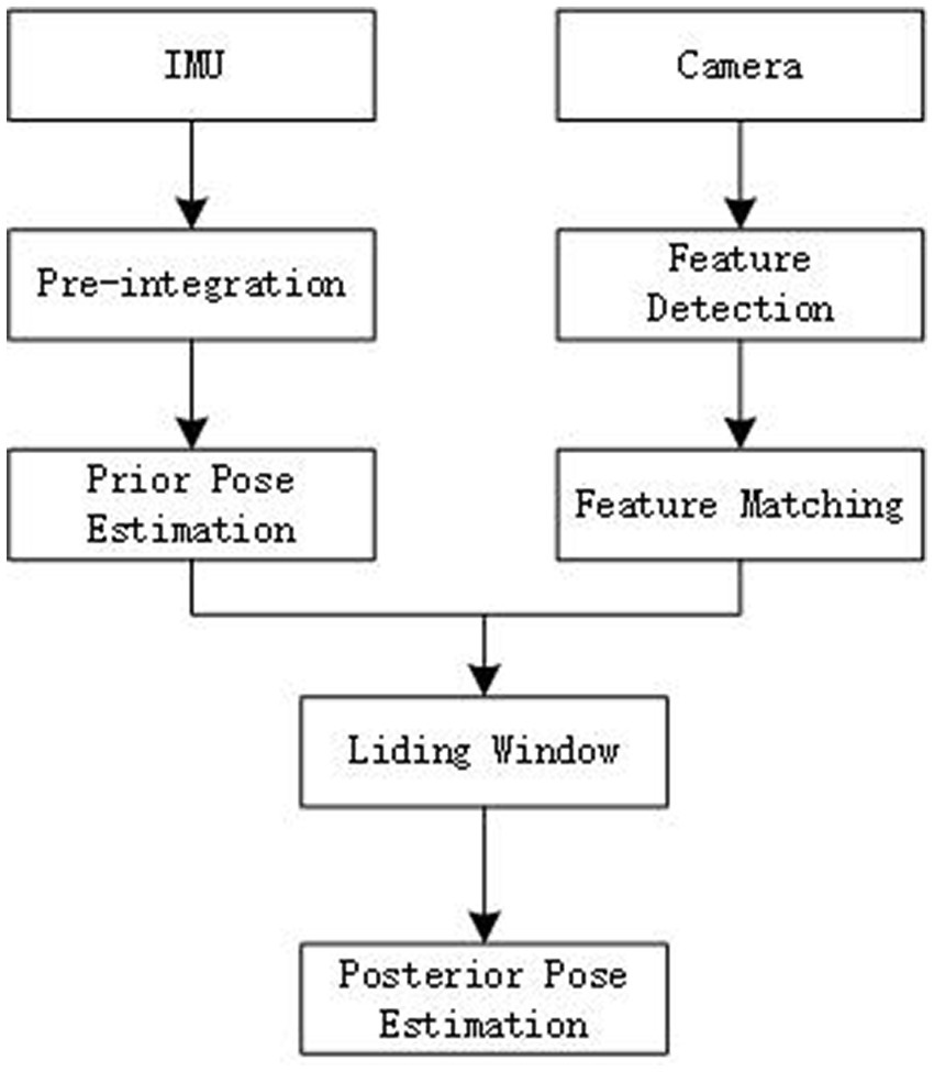
Figure 1. Front-end workflow.

Back end

After completing front-end pose estimation, the system enters back-end loop detection work. The Bag of Words method (BoW) is a popular appearance-based loop detection method (Angeli et al., 2008). The system uses the feature point description sub-sample of the observed environment image to obtain a dictionary through k-means training. Then, it checks whether a loop is formed by calculating word frequency (TF), inverse document frequency (IDF), and similarity calculation. Generally, when a loop is detected in multiple consecutive frames, it is considered that a loop is detected, and the pose transformation relationship (loop constraint) between the frame and the compared frame is calculated through feature matching, optimization, etc. Finally, new pose nodes and loop constraints are added to the keyframe pose graph, and the global pose can be corrected through graph optimization (Figure 2).

FIGURE 2

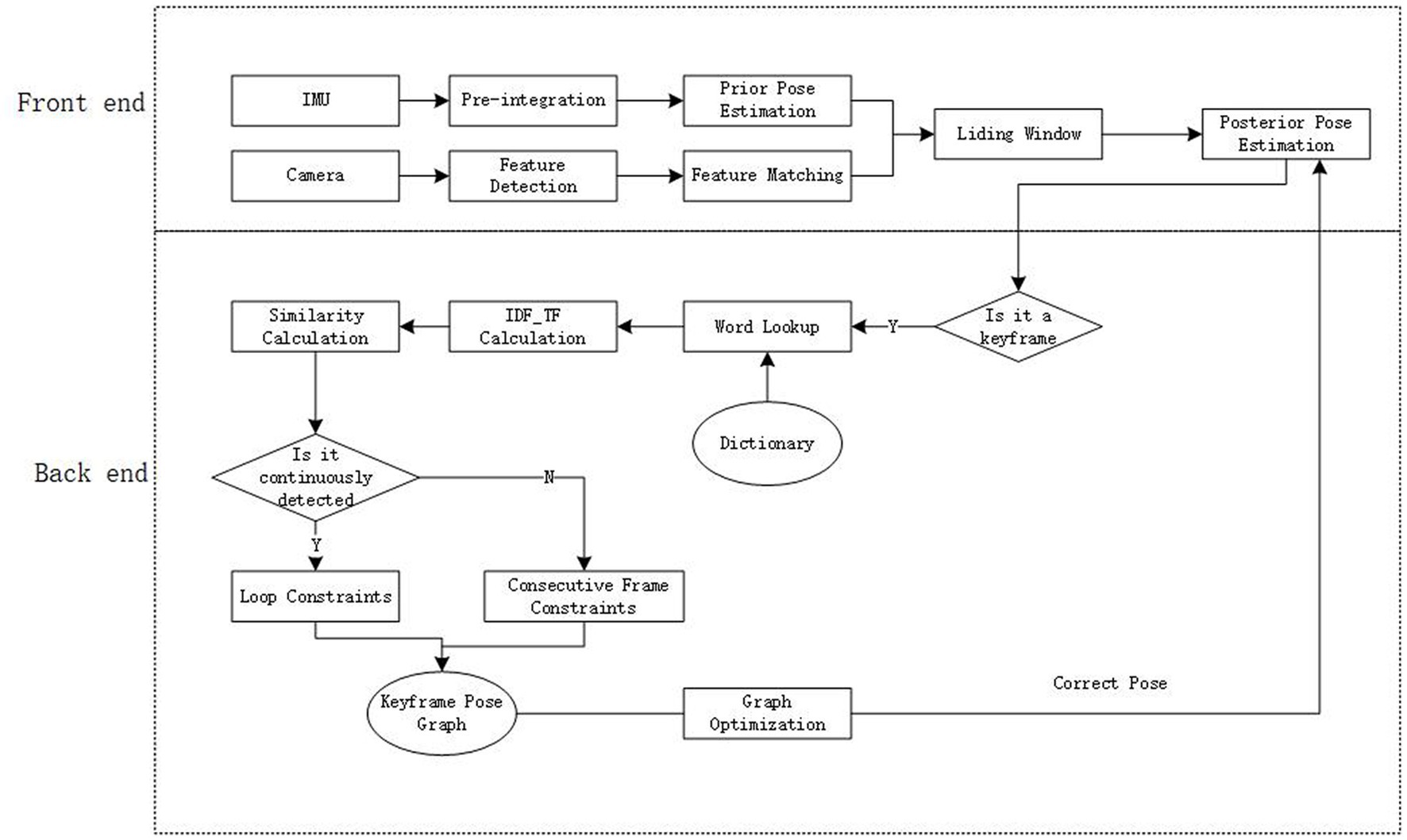
Figure 2. System workflow.

DBH and position calculation

The main difference between the DBH measurement function adopted in this study and the current forest survey using LiDAR SLAM lies in the real-time performance. With LiDAR SLAM, post-processing is required on the obtained point cloud data after scanning the plot, and additional work is needed to extract the DBH position. In contrast, this research is mainly based on the single-frame point cloud solution obtained by visual SLAM to calculate the diameter, position of the tree, and various forest parameters in real-time.

To obtain the DBH, the system first acquires more than three points at the height of the DBH of the tree and projects them onto the horizontal plane to obtain their plane coordinates. It then calculates the vertical bisector between two points and sets the corresponding weight coefficient according to the position. The center coordinates are calculated when the angle bisector intersects in pairs, and the weighted center plane coordinates, that is, the position coordinates, are determined according to the weight. Finally, the system uses the center coordinates and DBH height points to calculate the radius and its mean value to determine the cross-sectional area. Once the area is obtained, this value can be used to calculate the DBH.

System operation process

In this study, a mobile phone camera is used as the sensor in the SLAM system (Figure 3). The system acquires images and solved state data, and constructs a consistent point cloud map. Then, the single-tree volume factor is solved. The images and states are used to build 3D virtual scenes using OpenGL. By aligning the SLAM coordinate system with the OpenGL coordinate system, observers can view augmented reality (AR) scenes through the mobile phone screen (Figure 4). The AR scene can be interacted with through the screen in the following ways: (1) The plot boundary is constructed in the OpenGL coordinate system. When the observer approaches the plot boundary, the mobile phone screen displays the position of the plot boundary. (2) When measuring a tree, the observer clicks the position of the ground diameter and the position of the breast diameter on the mobile phone screen. This helps the system determine the point cloud at the diameter circle and fit the discrete point cloud in a circle. The measurement system consists of four parts: defining the sample coordinate system, constructing a globally consistent sparse map, measuring each tree, and calculating parameters. The operation flow is shown in Figure 5. The defined plot coordinate system describes the position of each tree in the plot. The construction of a globally consistent sparse map reduces the drift of the mobile phone pose obtained during measurement through loop detection, thereby reducing the estimation error of tree position. All trees in the sample plot are observed during the measurement of each tree. The parameter calculation process calculates the forest structural parameters of the area represented by the sample plot.

FIGURE 3

Figure 3. Measurement phone.

FIGURE 4

Figure 4. Different statuses of system during observation. (A) Determine the location of the plot center. (B) Sample boundaries. (C) Click on the position of the tree. (D) Click on the position of the DBH. (E) Overview of the sample. (F) Calculated forest structure parameters.

FIGURE 5

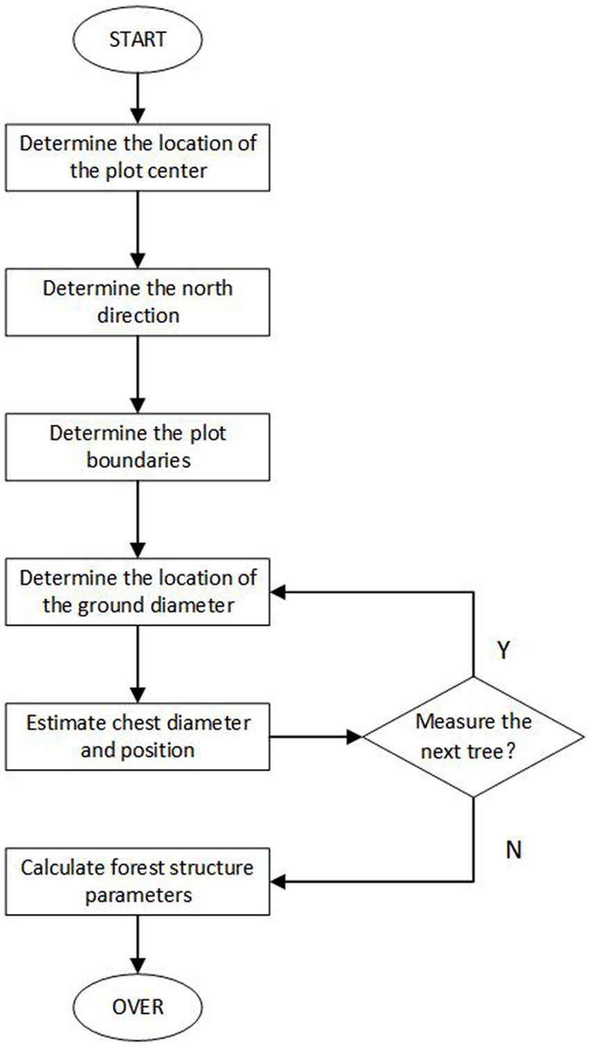
Figure 5. Workflow of forest inventory system.

SLAM operates through a process that is divided into four modules: front-end odometer, back-end optimization, loop closure detection, and map building. The loop closure detection module is crucial for refining data and correcting pose drift caused by the front-end visual odometer. Its main function is to detect similar data collected by the sensor at the same place, and use this information to ensure data consistency. The accuracy of the globally consistent map is closely related to the scan trajectory, and proper loop closure detection during the scanning process is essential for obtaining an accurate map. In this study, a fixed sample scan path was designed, starting at the center of the sample plot and measuring the trees along the route of progress, as shown in the Figure 6. Traditional SLAM systems with image feature-based backends may not work well in poorly constructed forests. Therefore, an online trunk-based backend was designed in this study to estimate tree position accurately and correct pose drift in real time for large-scale forest inventories. Specifically, a trunk-based loop closure detection algorithm was developed to detect whether an earlier observed tree is re-observed, providing nodes and constraints for tree position graph optimization. This algorithm builds and optimizes the tree position graph using the provided nodes and constraints, and corrects the current pose based on the optimized globally consistent tree position graph.

FIGURE 6

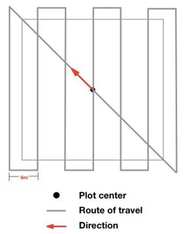
Figure 6. Scanning trajectory for building plot map.

Spatial parameter selection

The forest spatial structure index based on the relationship between adjacent trees has been widely used in the research of forest spatial structure analysis, competition and advantage calculation, species diversity measurement, forest structure reconstruction and management optimization. The spatial structural parameters are mainly a comprehensive expression of the single-tree volume factor and spatial position. The position of standing trees and the single-tree volume factor were measured by mobile phone measurement system to solve the spatial structural parameters, and the spatial structural parameters considered in this study mainly included Mingling degree, Dominance index, Uniform angle index, and Crowdedness index.

Mingling degree mainly describes the species composition and spatial pattern in the forest. It is defined as the proportion of individuals in the four nearest neighboring trees of the target tree i who are not of the same species as the target tree.

$M\mathrm{i}=\frac{1}{4}{\displaystyle \sum }_{j=1}^{4}vij$

${\mathrm{v}}_{\mathrm{ij}}=\left\{\begin{array}{c}\begin{array}{l}1,If\mathrm{}the\mathrm{neighboring\; tree}jand\mathrm{}the\mathrm{target}treei\\ aredifferent\mathrm{}species\end{array}\\ \begin{array}{l}0,If\mathrm{}the\mathrm{neighboring\; tree}jand\mathrm{}the\mathrm{target}treei\\ aresame\mathrm{}species\end{array}\end{array}\right.\text{ (6)}$

Uniform angle index describes the uniformity of adjacent trees around the reference tree i, and is defined as the proportion of the number of α angles less than the standard angle α₀ in the number of nearest neighboring trees. The standard angle α₀ is selected as 72° according to the research conducted by Hui et al. (2004).

$W\mathrm{i}=\frac{1}{4}{\displaystyle \sum }_{j=1}^4\mathrm{z}ij$

${\mathrm{z}}_{\mathrm{ij}}=\{\begin{array}{c}1,If\mathrm{}the\mathrm{\alpha }is\mathrm{}less\mathrm{}than\mathrm{}the{\mathrm{\alpha }}_0\\ 0,If\mathrm{}the\mathrm{\alpha }is\mathrm{}greater\mathrm{}than\mathrm{}or\mathrm{}equal\mathrm{}to{\mathrm{\alpha }}_0\end{array}\text{ (7)}$

The Dominance index quantitatively describes tree competition and is defined as the proportion of the adjacent trees of the reference tree whose DBH is greater than the number of reference trees to the four nearest neighbors examined.

$D\mathrm{i}=\frac{1}{4}{\displaystyle \sum }_{j=1}^4\mathrm{k}ij$

${\mathrm{k}}_{\mathrm{ij}}=\left\{\begin{array}{c}\begin{array}{l}1,If\mathrm{}the\mathrm{neighboring\; tree}jis\mathrm{}smaller\mathrm{}than\mathrm{}\\ the\mathrm{target}treei\end{array}\\ \begin{array}{l}0,If\mathrm{}the\mathrm{neighboring\; tree}jis\mathrm{}greater\mathrm{}than\mathrm{}\\ or\mathrm{}equal\mathrm{}to\mathrm{}the\mathrm{target}treei\end{array}\end{array}\right.\text{ (8)}$

The Crowdedness index describes the horizontal distribution pattern of tree positions and is defined as the ratio of the average distance of the nearest neighbor to the expected average distance under random distribution.

$\begin{array}{ll}R=\frac{\frac{1}{\mathrm{n}}{\displaystyle \sum }_{i=1}^{n}ri}{\frac{1}{2}\sqrt{\frac{S}{n}}}& (9)\end{array}$

r_i is the distance from the tree i to its nearest neighbor; n is the total number of plants in the plot; S is the sample area.

Study area and sample plots information

In this study, three plots of 32 m × 32 m were selected for testing, located in the campus forest area of Beijing Forestry University, the Olympic Forest Park, and Dongsheng Bajia Park in Beijing, China. Plot 1 is a mixed forest with Juniperus chinensis L. as the dominant tree species, while the other two plots are artificial pure forests dominated by Ginkgo biloba L. and Populus L. The three plots contain trees of different diameters, and the number and distribution of trees in each plot are different, which comprehensively tests the function of the measurement system. The sample plots have few shrubs and are convenient for data collection. The mobile phone measurement system was used to conduct the sample plot survey, and the spatial structure of the forest area was analyzed using the calculated spatial structural parameters. Additionally, the chest diameter and position data of the trees were recorded as reference data using a total station and a chest diameter ruler to test the accuracy.

Results

DBH accuracy

The diameter at breast height (DBH) of trees in the sample plot was estimated using a mobile phone measurement system, and the estimated values were compared to the true DBH obtained by measuring the trees with a diameter tape as a reference. In this study, the accuracy of DBH estimation was evaluated using the BIAS, RMSE, relative BIAS (relBIAS), and relative RMSE (relRMSE) metrics, which were calculated using the following formulas:

$\begin{array}{ll}{B}_{IAS}=\frac{{\displaystyle \sum }_{i=1}^n\left(x_i-x_{ir}\right)}{n}& (10)\end{array}$

$\begin{array}{ll}\mathrm{rel}B\mathrm{IAS}=\frac{{{\displaystyle \sum }}_{\mathrm{i}=1}^{\mathrm{n}}\left(xi/xir-1\right)}{\mathrm{n}}\times 100\%& (11)\end{array}$

$\begin{array}{ll}{R}_{MSE}=\sqrt{\frac{{\displaystyle \sum }_{i=1}^n{\left(x_i-x_{ir}\right)}^2}{n}}& (12)\end{array}$

$\begin{array}{ll}\mathrm{rel}RMSE=\sqrt{\frac{{{\displaystyle \sum }}_{\mathrm{i}=1}^{\mathrm{n}}{\left(xi/xir-1\right)}^2}{\mathrm{n}}}\times 100\%& (13)\end{array}$

where x_i is an estimate; x_ir is the reference value corresponding to x_i; n is the total number of trees.

The Figure 7A displays the overall distribution of DBH estimates for the three plots obtained using the mobile phone measurement system. The figure shows that all DBH estimates were close to the corresponding reference values, and there were no apparent abnormal estimates. This observation suggests that this method of estimating breast diameter is highly robust. Statistical analysis of all DBH estimates was performed, and the results are presented in Table 1.

FIGURE 7

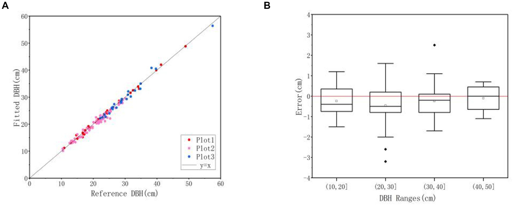
Figure 7. DBH estimates error statistics. (A) DBH estimates distribution. (B) The errors under different DBH ranges.

TABLE 1

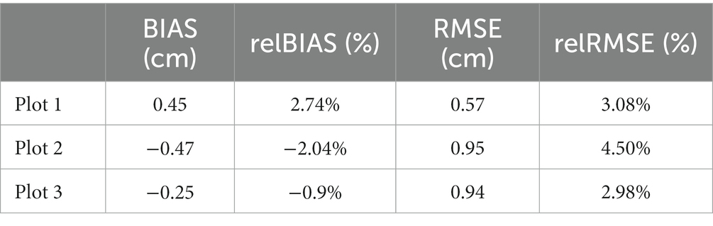
Table 1. Accuracies of the DBH estimates.

The DBH obtained through the mobile phone measurement system had a BIAS value close to zero, indicating that it was nearly unbiased (−0.47 ~ 0.45 cm, −2.04% ~ 2.74%) compared to the reference value obtained using the diameter tape. Moreover, the DBH estimates had small RMSEs overall (0.57 ~ 0.95 cm, 2.95% ~ 4.5%), as shown in Table 1. Figure 7B is a box plot of the error of the DBH estimates in different diameter steps, which indicates that the average error of the DBH estimate in different DBH ranges was close to zero. These results demonstrate that the mobile phone measurement system can achieve high-precision DBH measurement, and the measurement accuracy meets the requirements for further determining forest structural parameters.

Position accuracy

The measured tree position data for the three plots are shown in Figure 8. The overall deviation was small, and the estimated position could accurately reflect the actual position of the sampled trees. As shown in Table 2, the BIAS of the x-axis was −0.04 to 0.22 m and the y-axis was 0.01 to 0.20 m. The tree position estimates for the three plots had relatively small RMSEs of 0.17 to 0.22 m on the x-axis and 0.16 to 0.26 m on the y-axis. The scatter distribution of errors in the two axes was relatively uniform. Since the spatial structural parameters only require the determination of neighboring trees based on their position, and the position data was not calculated as a parameter, the position accuracy of the system fitting could meet the requirements for further spatial structural parameter calculations.

FIGURE 8

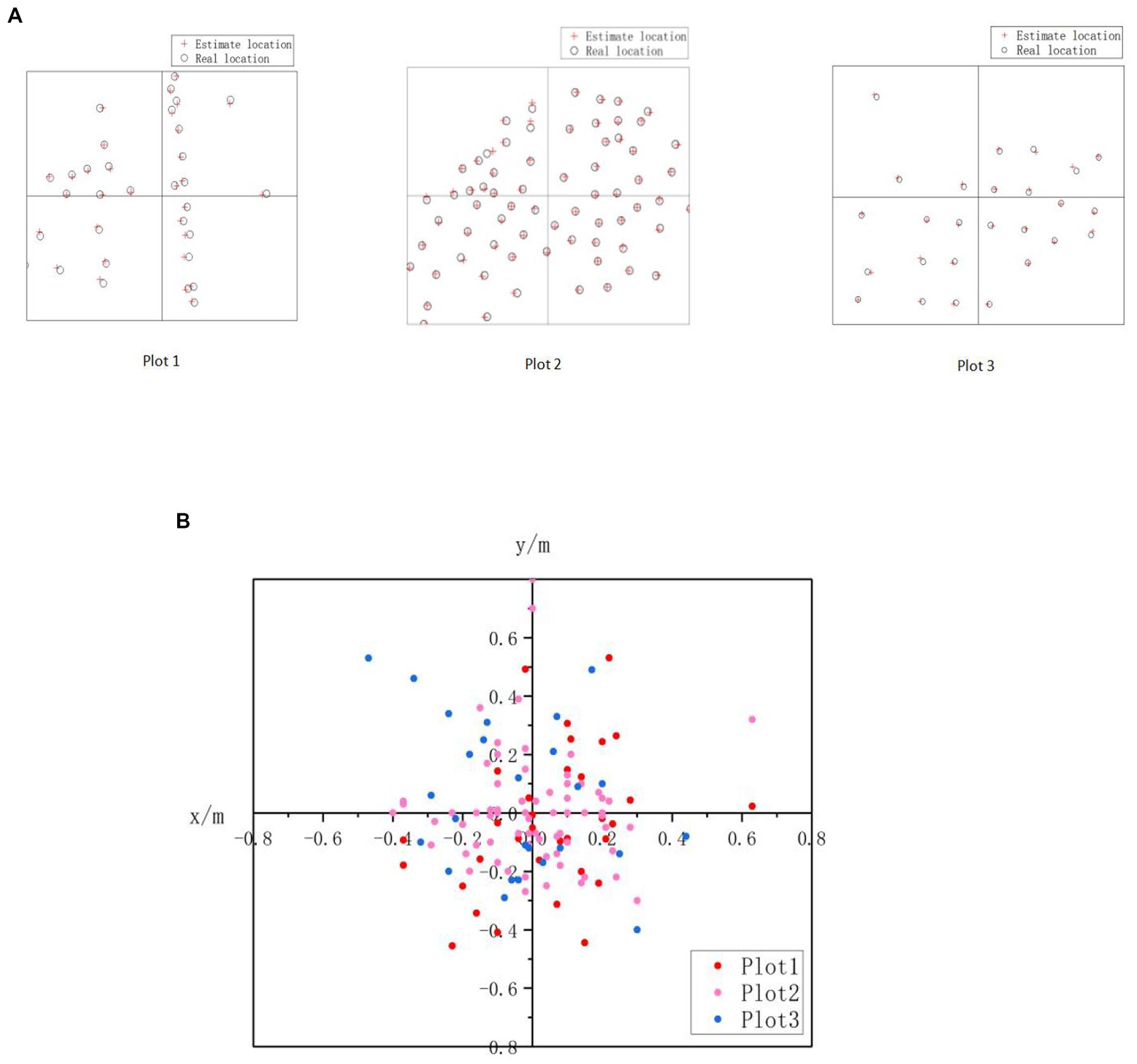
Figure 8. Position estimates error statistics. (A) Tree position distribution. (B) Position errors of all trees in plots.

TABLE 2

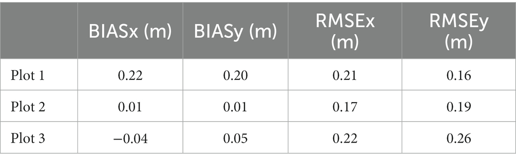
Table 2. Accuracies of the position estimates.

Spatial structural parameter calculation

The horizontal distance between trees was calculated based on the position coordinates, and the four nearest neighboring trees of each reference tree were determined based on their distances. By comparing the non-spatial structural parameters (such as DBH, tree species, and position distribution) of the reference tree and its neighboring trees, and applying the relevant formula, the spatial structural parameters of the forest area in the sample plot were calculated, including Mingling degree, Dominance index, Uniform angle index, and Crowdedness index. The value range and index system of each spatial parameter are presented in Table 3.

TABLE 3

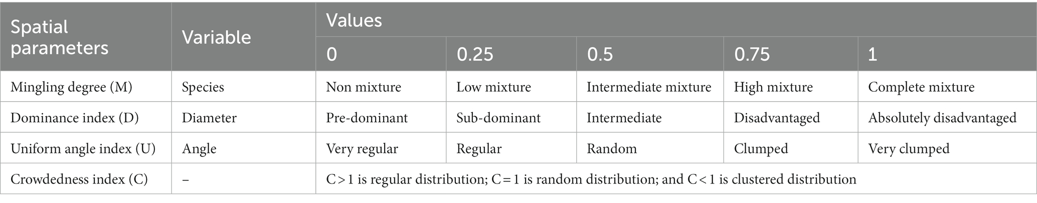
Table 3. Forest spatial structure index system.

The spatial distribution of each tree species in Plot 1 can be clearly seen in Figure 9, where it shows that Juniperus chinensis L. was the dominant tree species in the area. The parameter values of the forest stand are presented in Table 4, showing that the mixing degree of the whole forest stand was 0.32, which is considered weak. As both Plots 2 and 3 were single-species plots, their species distribution is not shown, and the mixing degree of both plots was 0. From Figure 10A, a relatively high percentage of 0 values can be observed, indicating that trees of the same species were clustered in Plot 1. This conclusion is also apparent from Figure 8, as trees of the same species in the sample plot had a higher degree of aggregation. The dominance index reflects the competition among forest trees, and the dominance index values for the three plots were 0.56, 0.51, and 0.51, suggesting that the competitive advantage of the whole forest species was not apparent, and tree growth was relatively balanced. The uniform angle index and crowdedness index describe the spatial distribution of trees in the forest area. The uniform angle index values for the three plots were 0.55, 0.59, and 0.61, indicating that the position of trees in the plots was randomly distributed. The crowdedness index is the ratio of the mean distance between the horizontal distance of the reference tree and the neighboring trees to the expected average distance. The crowdedness index for Plot 1 was 1.03, indicating that the degree of aggregation of the trees was low and showed a random distribution trend. The crowdedness index for Plots 2 and 3 were 1.36 and 1.40, respectively, suggesting that the trees in the plots showed a trend of uniform distribution, and the uniformity of Plot 3 was higher than that of Plot 2, but the overall uniformity was relatively weak.

FIGURE 9

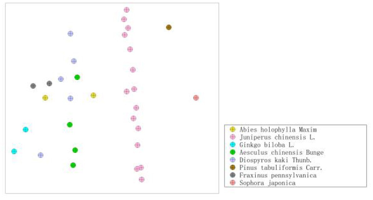
Figure 9. Spatial distribution of different tree species.

TABLE 4

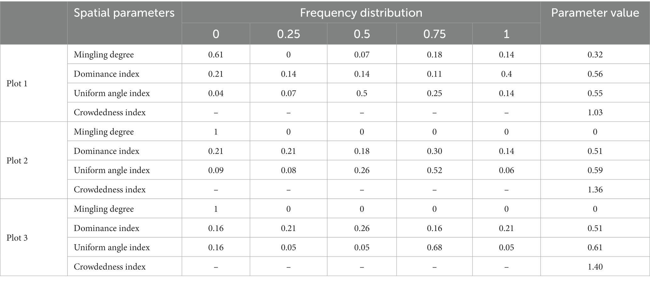
Table 4. Frequency values for different spatial structural parameters.

FIGURE 10

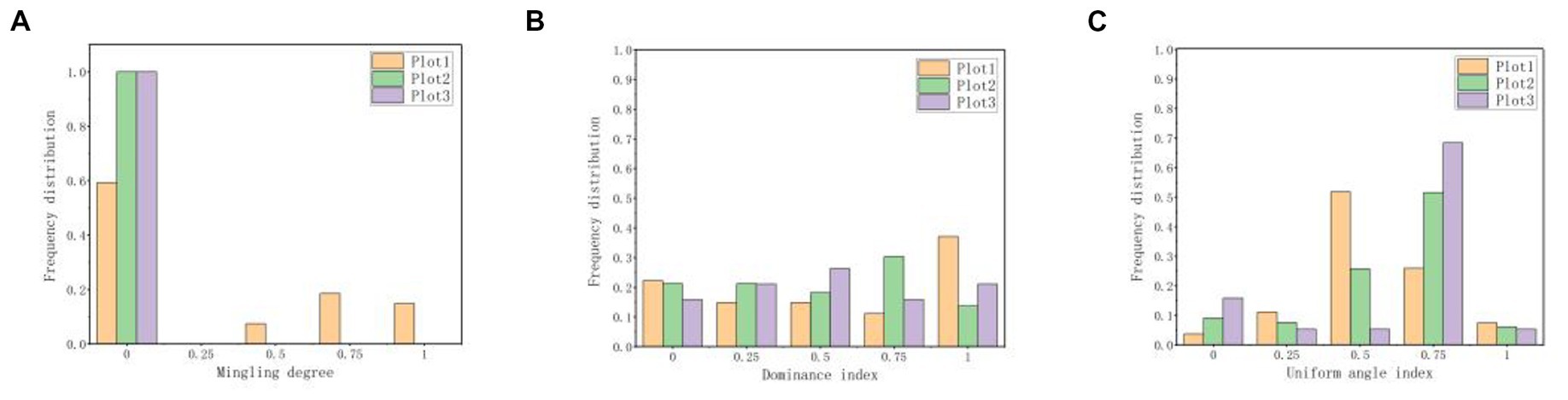
Figure 10. Frequency distribution of different spatial structural parameters. (A) Mingling degree. (B) Dominance index. (C) Uniform angle index.

Discussion

In recent years, the development of forestry inventory has been based on intelligence and precision. Obtaining point cloud data of forest plots is an essential method to construct a 3D forest model and invert forest structural parameters. At this stage, the construction of forest point clouds mainly uses LiDAR (TLS, MLS, HMLS, etc.) to register the point cloud with different algorithms and realize the construction of a complete point cloud map. Its core is to find the corresponding relationship between the initial point cloud and the target point cloud, transform the point cloud on the target object into the coordinate system, and convert the point cloud of the same target object scanned multiple times into the same coordinate system. The difference in the algorithm between LiDARs with different working methods lies in the use of different methods to obtain the corresponding relationship of point clouds at different times. The SLAM algorithm is an algorithm that obtains the position and attitude changes of the sensor during its movement and calculates the corresponding relationship of point clouds at different times according to the changes to realize the work of point cloud registration and map construction. Research on intelligent forestry survey tools is mainly concentrated on LiDAR, and they include (1) designing a multi-sensor fusion LiDAR system to improve the scanning range and improve the point cloud mapping effect, (2) designing and improving point cloud matching algorithms to obtain high-quality point cloud data, and (3) proposing a more efficient and accurate circle fitting method based on the original discrete point fitting DBH circle algorithm (e.g., least squares method, random sample consensus, and HoughCircles). These research efforts have greatly improved the efficiency and accuracy of forestry inventory.

However, lidar-based research still relies on computers for post-data processing and parameter extraction, which increases workload and reduces real-time performance. In this study, a measurement system was constructed on a mobile phone using visual SLAM+AR technology installed in the mobile phone camera to visually construct a sample site cloud map. This system got rid of the limitations of lidar for data collection, and real-time integrated measurement work was realized without requiring post-processing.

The results of the study show that the mobile phone measurement system can accurately solve the single-tree volume factor, meeting the needs of forestry inventory and providing high-quality data support for further solving other forest structural parameters. The system also allows for the investigation of forest spatial structure, which has become an increasingly important content of forestry investigation. The nearest neighbor method is an important means to calculate the parameters of the forest spatial structure. Using neighboring trees to investigate spatial structure parameters usually requires manual determination of neighboring trees to calculate parameters and assign values. This process is cumbersome and may cause errors due to subjective factors of the measurer. According to the position of the trees measured by this system, the four neighboring trees of the reference tree can be determined, and the spatial structural parameters of the forest can be preliminarily solved according to the relationship between the breast diameter and position of the reference tree and the neighboring tree. Therefore, by optimizing the forest inventory method, this study obtains the forest spatial structural parameters more efficiently, moreover, provides good data support for the study of forest ecology, and ultimately realizes the promotion of forest ecological management, optimization, and promotion of ecological sustainable development.

However, due to the performance gap between the mobile phone camera and the lidar, the current system based on vision has issues with its stability. The problem of pose drift occurs in actual use, and the stability and robustness of the system need to be improved. In the future, more measurement and auxiliary functions can be developed on mobile phones, including tree species recognition based on the surface characteristics of trunks or leaves and using point clouds to realize 3D modeling of trees. Overall, this system has high application value and broad development space in forestry inventory, as it optimizes the forest inventory method, provides good data support for the study of forest ecology, and ultimately promotes ecological sustainable development.

Conclusion

In this study, the mobile phone is used as a sensor, and the visual SLAM technology is used to replace the HMLS based on LiDAR SLAM, which improves the efficiency and portability. At the same time, the embedding of augmented reality technology realizes real-time measurement and can control errors well with high measurement accuracy of DBH and position, which can be used to determine the neighboring trees and calculate the spatial structural parameters of the forest areas. The test results show that the system can meet the inventory needs well and can be used as a new direction for future forest resources investigation and solving spatial structure parameters.

At this stage, there are still some problems in this study. The positioning method based on vision sometimes has positioning drift, and the stability still needs to be further improved. In addition, the number of system calculation parameters is currently limited, and in some surveys it is still necessary to rely on other tools for assistance, and more measurement functions need to be embedded in the future.

Data availability statement

The raw data supporting the conclusions of this article will be made available by the authors, without undue reservation.

Author contributions

FY conceived and designed the project. TG and MU wrote the manuscript. YF and FY conceptualized the study, designed the methodology, and reviewed the manuscript. LG conducted field experiments. All authors contributed to the article and approved the submitted version.

Funding

This work was supported by Tibet Autonomous Region Science and Technology Plan Project, project number: XZ202301YD0043C.

Acknowledgments

The authors would like to extend our sincere gratitude to the undergraduate students and staff of the Laboratory of Forest Management and “3S” technology and Beijing Forestry University for various help in the experimentation.

Conflict of interest

The authors declare that the research was conducted in the absence of any commercial or financial relationships that could be construed as a potential conflict of interest.

Publisher’s note

All claims expressed in this article are solely those of the authors and do not necessarily represent those of their affiliated organizations, or those of the publisher, the editors and the reviewers. Any product that may be evaluated in this article, or claim that may be made by its manufacturer, is not guaranteed or endorsed by the publisher.

References

Angeli, A., Doncieux, S., Meyer, J. A., and Filliat, D. Real-time visual loop-closure detection. In 2008 IEEE International Conference on Robotics and Automation. IEEE, (2008). 1842–1847.

Google Scholar

Bailey, T., and Durrant-Whyte, H. (2006). Simultaneous localization and mapping (SLAM). Part II. IEEE Robotics and Automation Magazine, 13108–117. doi: 10.1109/MRA.2006.1678144

CrossRef Full Text | Google Scholar

Bauwens, S., Bartholomeus, H., Calders, K., and Lejeune, P. (2016). Forest inventory with terrestrial LiDAR: a comparison of static and hand-held Mobile laser scanning. Forests 7:127. doi: 10.3390/f7060127

CrossRef Full Text | Google Scholar

Bienert, A., Scheller, S., Keane, E., Mullooly, G., and Mohan, F. (2006). Application of terrestrial laser scanners for the determination of forest inventory parameters. Int. Arch. Photogram. Remote Sens. Spatial Inform. Sci. :36, 1–5.

Google Scholar

Božić, M., Čavlović, J., Lukić, N., Teslak, K., and Kos, D. (2005). Efficiency of ultrasonic vertex III hypsometer compared to the most commonly used hypsometers in Croatian forestry. Croatian J. For. Eng. J. Theory Appl. Forest. Eng. 26, 91–99.

Google Scholar

Dong, L., Bettinger, P., and Liu, Z. (2022). Optimizing neighborhood-based stand spatial structure: four cases of boreal forests. For. Ecol. Manag. 506:119965. doi: 10.1016/j.foreco.2021.119965

CrossRef Full Text | Google Scholar

Fan, Y., Feng, Z., Chen, P., Gao, X., and Shen, C. (2019). Research on Forest plot survey system based on RGB-D SLAM Mobile phone. J. Agric. Mech. 50, 226–234. doi: 10.6041/j.issn.1000-1298.2019.08.024, in Chinese.

CrossRef Full Text | Google Scholar

Feng, Z. K., Han, X. C., Zhou, K. L., Nan, Y. T., and Fu, X. (2003). The analysis of forestry mensuration principle and precision in fixed samples by total station. Beijing Surv. 2003, 28–30. in Chinese.

Google Scholar

Gao, W., Lei, X., Liang, M., Larjavaara, M., Li, Y., Gao, D., et al. (2021). Biodiversity increased both productivity and its spatial stability in temperate forests in northeastern China. Sci. Total Environ. 780:146674. doi: 10.1016/j.scitotenv.2021.146674

PubMed Abstract | CrossRef Full Text | Google Scholar

Gui, J., Gu, D., Wang, S., and Hu, H. (2015). A review of visual inertial odometry from filtering and optimisation perspectives. Adv. Robot. 29, 1289–1301. doi: 10.1080/01691864.2015.1057616

CrossRef Full Text | Google Scholar

Heidenreich, M. G., and Seidel, D., (2022). Assessing Forest vitality and Forest structure using 3D data: A case study from the Hainich National Park, Hainich: Frontiers in Forests and Global Change.

Google Scholar

Hu, G., Khosoussi, K., and Huang, S.. Towards a reliable SLAM back-end. 2013 IEEE/RSJ International Conference on Intelligent Robots and Systems. IEEE, (2013). 37–43.

Google Scholar

Hui, G., and Gadow, G. (2003). Quantitative analysis of forest spatial structure. Beijing: Science and Technology Press.

Google Scholar

Hui, G., Gadow, K., and Hu, Y. (2004). Standard angle selection of angular scale of Forest stand spatial structure parameters. For. Res. 2004, 1001–1498. doi: 10.3321/j.issn:1001-1498.2004.06.001, (in Chinese).v

CrossRef Full Text | Google Scholar

Hui, G., Li, L., Zhao, Z., and Dang, P. (2007). Comparison of methods in analysis of the tree spatial distribution pattern. Acta Ecol. Sin. 27, 4717–4728. doi: 10.1016/S1872-2032(08)60008-6

CrossRef Full Text | Google Scholar

Hui, G., Zhang, G., Zhao, Z., and Yang, A. (2019). Methods of Forest structure research: a review. Curr. Forest. Rep. 5, 142–154. doi: 10.1007/s40725-019-00090-7

CrossRef Full Text | Google Scholar

James, M. R., and Quinton, J. N. (2014). Ultra-rapid topographic surveying for complexenvironments: the hand-held mobile laser scanner (HMLS). Earth Surf. Process. Landforms 39, 138–142. doi: 10.1002/esp.3489

CrossRef Full Text | Google Scholar

Leutenegger, S., Lynen, S., Bosse, M., Siegwart, R., and Furgale, P. (2015). Keyframe-based visual–inertial odometry using nonlinear optimization. Int. J. Robot. Res. 34, 314–334. doi: 10.1177/0278364914554813

CrossRef Full Text | Google Scholar

Li, M., and Mourikis, A. I.. Improving the accuracy of EKF-based visual-inertial odometry. 2012 IEEE international conference on robotics and automation. IEEE, (2012). 828–835.

Google Scholar

Li, M., and Mourikis, A. I. (2013). High-precision, consistent EKF-based visual-inertial odometry. Int. J. Robot. Res. 32, 690–711. doi: 10.1177/0278364913481251

CrossRef Full Text | Google Scholar

Liang, X., Hyyppä, J., Kukko, A., Kaartinen, H., Jaakkola, A., and Yu, X. (2014). The use of a Mobile laser scanning system for mapping large Forest plots. IEEE Geosci. Remote Sens. Lett. 11, 1504–1508. doi: 10.1109/LGRS.2013.2297418

CrossRef Full Text | Google Scholar

Liang, X., Kankare, V., Hyyppä, J., Wang, Y., Kukko, A., Haggrén, H., et al. (2016). Terrestrial laser scanning in forest inventories. ISPRS J. Photogramm. Remote Sens. 115, 63–77. doi: 10.1016/j.isprsjprs.2016.01.006

CrossRef Full Text | Google Scholar

Lim, K., Treitz, P., Wulder, M., St-Onge, B., and Flood, M. (2003). LiDAR remote sensing of forest structure. Progr. Phys. Geogr. Earth Environ. 27, 88–106. doi: 10.1191/0309133303pp360ra

CrossRef Full Text | Google Scholar

Maas, H. G., Bienert, A., Scheller, S., and Keane, E. (2008). Automatic forest inventory parameter determination from terrestrial laser scanner data. Int. J. Remote Sens. 29, 1579–1593. doi: 10.1080/01431160701736406

CrossRef Full Text | Google Scholar

Murphy, G. E., Acuna, M. A., and Dumbrell, I. (2010). Tree value and log product yield determination in radiata pine (Pinus radiata) plantations in Australia: comparisons of terrestrial laser scanning with a forest inventory system and manual measurements. Can. J. For. Res. 40, 2223–2233. doi: 10.1139/X10-171

CrossRef Full Text | Google Scholar

Pastorella, F., and Paletto, A. (2013). Stand structure indices as tools to support forest management: an application in Trentino forests (Italy). J. Forest Sci. 59, 159–168. doi: 10.17221/75/2012-JFS

CrossRef Full Text | Google Scholar

Rublee, E., Rabaud, V., Konolige, K., and Bradski, G. (2011). ORB: an efficient alternative to SIFT or SURF. Int. Conf. Comp. Vis. 2011:107.

Google Scholar

Ryding, J., Williams, E., Smith, M. J., and Eichhorn, M. P. (2015). Assessing handheld mobile laser scanners for forest surveys. Remote Sens. 7, 1095–1111. doi: 10.3390/rs70101095

CrossRef Full Text | Google Scholar

Tang, M. (2010). Advances in study of Forest spatial structure. Scientia Silvae Sinicae 46, 117–122. (in Chinese).

Google Scholar

Vastaranta, M., Melkas, T., Holopainen, M., Kaartinen, H., Hyyppä, J., and Hyyppä, H. (2009). Laser-based field measurements in tree-level forest data acquisition. Photogram. J. Finland 21, 51–61.

Google Scholar

Yan, F., Mohammad, R. U., Gong, Y., Feng, Z., Chowdury, Y., and Wu, L. (2012). Use of a no prism total station for field measurements in Pinus tabulaeformis Carr. Stands in China. Biosyst. Eng. 113, 259–265. doi: 10.1016/j.biosystemseng.2012.08.007

CrossRef Full Text | Google Scholar