 Nathan J. Kleist1*Kurt M. Fristrup2Rachel T. Buxton3Megan F. McKenna4Jacob R. Job5Lisa M. Angeloni5Kevin Crooks1George Wittemyer1
- 1Department of Fish, Wildlife, and Conservation Biology, Colorado State University, Fort Collins, CO, United States
- 2Department of Electrical and Computer Engineering, Colorado State University, Fort Collins, CO, United States
- 3Department of Biology, Institute of Environmental and Interdisciplinary Sciences, Carleton University, Ottawa, ON, Canada
- 4Hopkins Marine Station of Stanford University, Pacific Grove, CA, United States
- 5Department of Biology, Colorado State University, Fort Collins, CO, United States
Anthropogenic noise sources impact ecological processes by altering wildlife behavior and interactions with cascading impacts on community structure. The distribution and magnitude of such noise has grown exponentially over the past century, and now inundates even remote areas. Here we investigate biological responses to prolific, anthropogenic noise sources associated with the physical presence of the source (vehicle noise and human voices) and disconnected from it (aircraft overflight). Bioacoustic responses to these noise sources were documented at 103 sites in 40 U. S. National Park units. The presence of bird sounds was noted in 10-s audio samples every 2 min, for 8 days at each site and related to the presence of human voices, vehicle noise, and aircraft noise in the same and preceding samples. Generalized additive models were used to fit smoothing splines to weight the influence of noise in past samples on the probability of detecting bird sounds in the present sample. We found that the probability of hearing birds increased immediately following noise events, and decreased about 2 h after the event. The negative effects were persistent more than 3 h after a noise event. The persistence of these responses – especially for noise from jets that were many kilometers distant – raises questions about the functional significance and ecological consequences of this altered activity, particularly in light of the widespread and diverse habitats in this study and ubiquity of the noise sources evaluated.
Introduction
Anthropogenic noise is increasingly recognized as a key stressor in ecological systems. Influential studies contrasting urban and wildland bird songs (Slabbekoorn and Peet, 2003), ecological studies exploring industrialized wildland settings (Habib et al., 2007; Francis et al., 2009), and field experimental playback studies (McClure et al., 2013) stimulated a growing body of evidence documenting myriad impacts of noise on natural systems. In addition to these specific studies, evidence concerning noise exposures and its ecological effects has been documented on continental scales (Mennitt et al., 2014; Senzaki et al., 2020; Wilson et al., 2021). Yet, two avenues of inquiry have been underserved: (1) how do wildlife responses change as time passes after a transient noise (and what are the combined effects of sequences of transient noises), and (2) what are the relative roles of lost auditory awareness and perception of a proximal threat in wildlife responses to noises?
Ecological responses to transient noise are likely to extend beyond the end of the event for several reasons. When noise induces physiologic stress (Kleist et al., 2018), the response can take many tens of minutes to return to baseline hormone levels, with longer intervals associated with unfamiliar stressors and unfavorable outcomes from the event (Koolhaas et al., 2011; Herman et al., 2016). Noise may change production of ‘contagious’ songs and calls, so restoration of previous vocal rates would depend upon social dynamics. Noise degrades the integrity of ecological auditory scenes; individuals likely require time to reestablish confidence in their auditory surveillance. Yet studies of the time course of behavioral responses to noise events are sparse. Behavioral responses extending more than an hour past exceptionally loud, transient acoustic stimuli have been observed in waterfowl (Goudie and Jones, 2004) and humpback whales (Fristrup et al., 2003).
The proximity of most terrestrial noise sources raises the possibility that responses to noise may depend upon the threat presented by the presence of the object producing the noise. Even in recent studies of “phantom” road noises, organismal responses could plausibly be conditioned by prior experience of vehicles and the hazards they present (McClure et al., 2013, 2017). This potential confound motivated studies of chronic energy development noise using observational designs that contrasted ecological conditions between matched sites differing only in noise exposure (Habib et al., 2007; Bayne et al., 2008; Francis et al., 2009).
Noise could either increase or decrease bioacoustic activity (Sun and Narins, 2005). Animals may become still and silent (Watkins and Schevill, 1975; Dapper et al., 2011; Tyack et al., 2011), especially when noise evokes perception of a high threat level. This makes individuals less conspicuous and enables more sensitive listening. Alternatively, some animals may become more vocal for several reasons. Transient noise can directly stimulate vocalization. Animals may compensate for the masking effects of noise with louder and more frequent vocalization (Brumm and Slater, 2006; Brumm and Zollinger, 2011). Animals may compensate for reduced auditory awareness by increasing call rates (Kaiser and Hammers, 2009) or eliciting social cooperation for predator surveillance (Uster and Zuberbüler, 2001).
Acoustic monitoring offers opportunities to document transient noises and bioacoustic responses to them. The Natural Sounds and Night Skies Division (NSNSD) of the U.S. National Park Service (NPS) accumulated an enormous archive of audio recordings and analyzed them to document types of noise and ecological sounds. A recent comprehensive assessment of NSNSD data indicate that the top three noise sources from U.S. National Parks were aircraft noise (mostly high-altitude jets), vehicle noise, and sounds from people (e.g., voices, footsteps; Buxton et al., 2019). Using the same dataset, we assess (1) if avian community sounds change with exposure to transient noises, (2) the time progression of any changes detected, and (3) if the responses to the three noise sources differ.
Methods
Collection of acoustic data
We analyzed acoustic data from 103 NPS sites within 40 National Park units across the conterminous United States (Figure 1) that was collected between 2010 and 2017 by NSNSD to monitor acoustic conditions. Site selection was non-random, seeking to identify locations representative of zones of management interest in each park and to diversify the NSNSD archive of monitored locations. Acoustic data were collected using ANSI Type 1 sound level meters (SLMs) and shrouded, 1.27 cm measurement microphones 1.5 m above the ground. The SLM generated calibrated 1 s, 1/3rd octave band spectra. The microphone and preamplifier systems for these units had a noise floor of 17 dB (A-weighted), except for very few remote sites where lower noise systems were used. To enable identification of sound events, the audio from the SLM was fed to an audio recorder. Digital audio recorders changed over time, with the Roland R-05 being the most recent device in our sample (Buxton et al., 2019). Differences in noise floors among audio recorders had negligible effect in the “active space” of the monitoring systems, as the recorders were fed amplified signals from the SLM. Input amplification levels were fixed for each type of recorder. Recorders differed in peak recordable sound levels, but if events exceeded these levels they could be reliably identified from the distorted audio and 1/3rd octave band spectra.
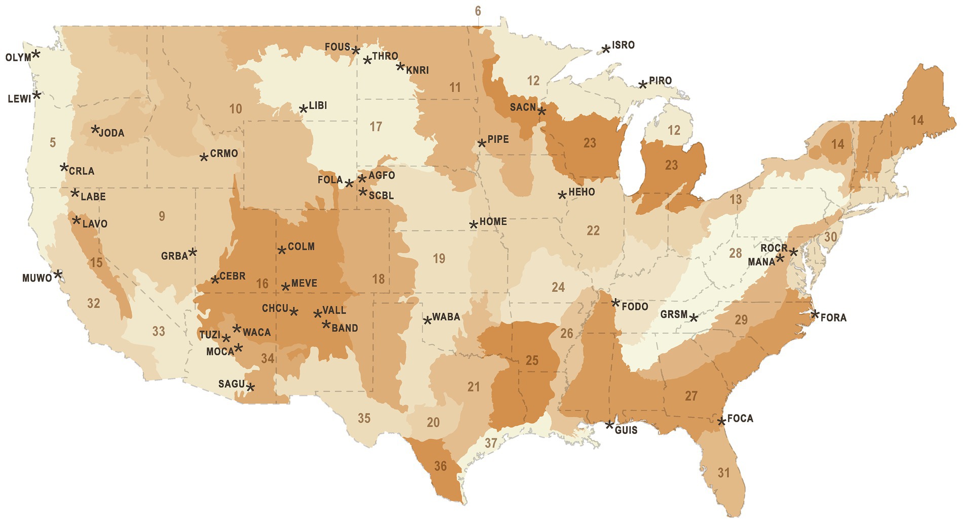
Figure 1. National Park units (black text and asterisks) and Bird Conservation Regions (numbered, shaded areas). National Park unit abbreviations are Agate Fossil Beds National Monument (AGFO), Bandelier National Monument (BAND), Cedar Breaks National Monument (CEBR), Chaco Culture National Historical Park (CHCU), Colorado National Monument (COLM), Crater Lake National Park (CRLA), Craters of the Moon National Monument (CRMO), Fort Caroline National Memorial (FOCA), Fort Donelson National Battlefield (FODO), Fort Laramie National Historic Site (FOLA), Fort Raleigh National Historic Site (FORA), Fort Union Trading Post National Historic Site (FOUS), Great Basin National Park (GRBA), Great Smoky Mountains National Park (GRSM), Gulf Islands National Seashore (GUIS), Herbert Hoover National Historic Site (HEHO), Homestead National Monument of America (HOME), Isle Royale National Park (ISRO), John Day Fossil Beds National Monument (JODA), Knife River Indian Villages National Historic Site (KNRI), Lava Beds National Monument (LABE), Lassen Volcanic National Park (LAVO), Lewis and Clark National Historical Park (LEWI), Little Bighorn Battlefield National Monument (LIBI), Manassas National Battlefield Park (MANA), Mesa Verde National Park (MEVE), Montezuma Castle National Monument (MOCA), Muir Woods National Monument (MUWO), Olympic National Park (OLYM), Pipestone National Monument (PIPE), Pictured Rocks National Lakeshore (PIRO), Rock Creek Park (ROCR), Saint Croix/Lower St. Croix National Scenic River (SACN), Saguaro National Park (SAGU), Scotts Bluff National Monument (SCBL), Theodore Roosevelt National Park (THRO), Tuzigoot National Monument (TUZI), Valles Caldera National Preserve (VALL), Washita Battlefield National Historic Site (WABA), Walnut Canyon National Monument (WACA). Bird Conservation Region numbers are Northern Pacific Rainforest (5), Boreal Taiga Plains (6), Great Basin (9), Northern Rockies (10), Prairie Potholes (11), Boreal Hardwood Transition (12), Lower Great Lakes/ St. Lawrence Plain (13), Atlantic Northern Forest (14), Sierra Nevada (15), Southern Rockies/Colorado Plateau (16), Badlands And Prairies (17), Shortgrass Prairie (18), Central Mixed Grass Prairie (19), Edwards Plateau (20), Oaks And Prairies (21), Eastern Tallgrass Prairie (22), Prairie Hardwood Transition (23), Central Hardwoods (24), West Gulf Coastal Plain/Ouachitas (25), Mississippi Alluvial Valley (26), Southeastern Coastal Plain (27), Appalachian Mountains (28), Piedmont (29), New England/Mid-Atlantic Coast (30), Peninsular Florida (31), Coastal California (32), Sonoran And Mojave Deserts (33), Sierra Madre Occidental (34), Chihuahuan Desert (35), Tamaulipan Brushlands (36), Gulf Coastal Prairie (37), Sierras De Baja California (39).
Identifying sounds in acoustic data
Trained acoustic technicians at Colorado State University analyzed the acoustic data. Earlier data sets were analyzed by salaried research associates, all of whom had graduate degrees in biology or acoustics. The research associates were trained by NPS staff. The later data were analyzed by salaried undergraduates supervised by a postdoctoral expert. The undergraduates were trained on two different datasets prior to analyzing data on their own. One data set was from a wilderness site that was acoustically characteristic of many of NPS backcountry locations. The second data set was from an urban park and included most of the anthropogenic noises that were present in monitoring data. Students analyzed each data set and reviewed their results with the postdoctoral expert, repeating sections when their results did not match with the expert’s results (which were developed using more intensive scrutiny and analysis). Coaching included ways to improve the student’s ability to correctly identify sounds by ear and with the use of an associated spectrogram. This training took from 2 to 5 weeks, depending on each student’s aptitude and prior experience.
The postdoctoral expert reviewed a segment of every site’s data prior to assigning projects to students. They briefed the students to make them aware of typical and challenging sounds that were present in the data set. Each site’s data were analyzed by at least two students. Both students analyzed 2 days of the same data to enable them to compare their results and ensure that they reached a consensus on how sounds were identified for that site.
At least eight 24-h days per monitoring site were analyzed: five weekdays and three weekend days. Days were selected at random, after eliminating days with wind speeds that exceeded 5 m/s (gusts could exceed 5 m/s) and days when staff visited the site. For days that were analyzed, 10 s segments of audio were examined every 2 min, yielding 720 records of identified sound sources per day.
Sound source identification was initiated by visual inspection of continuous, 1/3rd octave spectrograms spanning 12 Hz to 20 kHz using the Acoustic Monitoring Toolbox software developed by the National Park Service (NSNSD, 2013). The SLM spectrograms provided adequate detail to resolve most anthropogenic noise sources, but bioacoustic sounds were less readily identified. All ambiguous spectrogram signatures were reviewed with focused listening to corresponding audio files. For noise sources, results from visual and auditory review of acoustic data have been shown to be comparable (Lynch et al., 2011). Audio review was conducted with noise canceling headphones to diminish the influence of varying office noise on results.
Standardized codes were utilized to characterize broad categories of sounds (e.g., aircraft, vehicle, people talking, bird, mammal, wind, rain; for more detail see Buxton et al., 2019). Up to six codes were entered for each 10-s period (NSNSD, 2013). When more than six sources were identified, the first six were used. 0Though different types of sounds were coded for many sound sources, in this analysis all codes for each noise source were collapsed into one summary category. For these data, aircraft noise was mainly high altitude jets (73%); road noise was almost entirely automobiles and motorcycles; people sounds were mainly voices (89%) (Buxton et al., 2019). The sample size used in this analysis was 741,600 10-s observations.
Noise interferes with human capacity to hear other sounds. The noises in this analysis have energy concentrated in low-frequency bands, below 1 kHz. The biologic sounds in this analysis occurred at higher frequencies, mostly above 1 kHz. This reduces, but does not eliminate, the masking effect of noise for human listeners.
Modeling noise exposure histories
The presence of bird sounds in each sample was modeled using a generalized additive model (GAM) with a logit link function (Table 1). The covariates included in the model were spline functions representing week of year, sun position, and histories of exposure to noise from vehicles, aircraft, and people (aggregated presence of noise in samples up to 3 h previous).
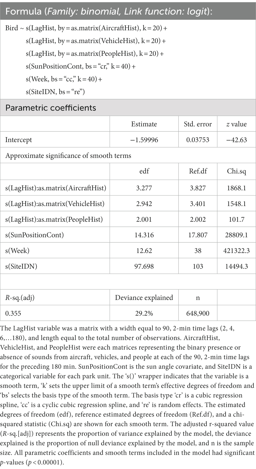
Table 1. Summary output for the full general additive model that was fit with data from all park units.
The noise exposure splines fitted smoothed weights to the recent binary history of detections (Wood, 2017) — a procedure that circumvented arbitrary decisions regarding time windows for summarizing noise exposure. From a signal processing perspective, this spline could be viewed as a smoothed finite impulse response (FIR) filter that was applied to the time series of noise presence/absence data. We expected the smoothed weights to decrease in magnitude with increasing temporal separation from the present observation, but these splines allow the possibility of latency between exposure and response.
To set up noise exposure histories for each observation, we prepared vectors of the 90 previous observations for each of the three sound sources. The presence of the noise source was encoded as a binary value (1 = noise present; see the variables AircraftHist, VehicleHist, and PeopleHist in Table 1). The spline fitted smoothed weights that multiplied each binary historical entry. The sum of these weighted histories provided an optimal fit to the data, in conjunction with the other terms in the model. Days of available observations were usually not consecutive, so assembly of these noise histories began each day at 00:00. Therefore, we could not investigate responses to noise during the first 3 h of each day (00:00 to 03:00), so the number of acoustic observations included in the models was 649,530.
The GAM was fitted using function bam() in the R package “mgcv” (Wood, 2021). The noise splines incorporated the exposure histories using the “by=” argument. The fitting process adjusted smoothed weights wi, to maximize the fit of the aggregate exposure factor ∑90j=1wj∗Hi,j , where Hi,j are binary values denoting the presence of noise in the jth 2-min interval preceding the ith observation. We used thin plate regression splines, with a basis dimension of 20. The basis dimension sets the upper limit of a smooth term’s effective degrees of freedom (EDF), which controls the extent of nonlinearity that can be fitted (Pedersen et al., 2019). To select smooth functions that result in the most parsimonious models, we used the function choose.k() from R package “mgcv” and followed the procedures in the associated documentation.
Modeling additional factors
Diel and annual changes in bird activity were modeled with additive spline terms. A cyclic cubic regression spline and a cubic regression spline, both with basis dimensions of 40, were used to generate smooth terms for week of year and sun angle above the horizon, respectively. We used the R package “lubridate” to calculate “Week” (from 1 to 52) (Grolemund and Wickham, 2011). The week of year smooth term accounted for annual variation in bird singing activity. The getSunlightPosition function from the R package “suncalc” (Thieurmel, 2022) was used to calculate the sun angle in radians relative to the horizon for each survey date, time, latitude, and longitude. We then created a sunlight position variable by matching the raw sun angle through the highpoint in the sky, then increasing the angles after solar noon by the absolute value of the change in sun angle from solar noon. This synthetic sun position variable distinguished dawn and dusk light conditions that are known to drive daily patterns in avian vocal behavior (Aschoff, 1966). Finally, we included a random effect for “Site,” which allowed the model to accommodate different group means for each site.
As model selection procedures rarely remove smooth terms from a model, we used automatic smooth term selection in bam() to identify the optimal number of smooth terms. Smooth term selection imposed a selection penalty on smooth terms that constrained model complexity (Marra and Wood, 2011). Fits of smooth terms were constrained in bam() by setting the gamma parameter equal to half the natural logarithm of the sample size. We fit models with the bam default method fREML (“fast REML”), and discretized covariates for efficiency. We also accounted for temporal autocorrelation in the response variable using the R package “itsadug” (Van Rij et al., 2015). We fit the full model without a first order autoregressive (AR1) model and used the function start_value_rho() to extract the AR1 correlation parameter. We then set the start of each time series as the beginning of each unique day of recordings for each year and site and refit the model with the AR1 term.
Bird conservation regions
Bird Conservation Regions (BCRs) are ecologically distinct North American regions with similar bird communities and biotic and abiotic characteristics that were developed by the North American Bird Conservation Initiative to promote a regional approach to bird conservation (Figure 1). We extracted the corresponding BCR unit for each site from a polygon layer made available by Bird Studies Canada (NABCI, 2014), and then subset the full dataset (n = 741,600) by BCR. The BCR models were identical to the full model, with the exception that the ‘week’ covariate was replaced by ‘day of year’. We ran separate model selection procedures for each BCR, to investigate the consistency of modeled responses to different anthropogenic noise sources.
Results
Statistical summaries of the observations
Aircraft sounds were detected in 14.2% of all samples (n = 741,600) with a high of 40.0% at Rock Creek National Park (ROCR) and a low of 1.3% at Homestead National Monument of America (HOME) (Figure 2). Vehicles sounds were detected in 21.4% of all samples with a high of 99.1% at Herbert Hoover National Historic Site (HEHO, which is adjacent to Interstate 80 in Iowa) and a low of 0.1% at Lewis and Clark National Historic Park (LEWI). Sounds from people were detected in 6.5% of all samples, with a high of 40.5% at Muir Woods National Monument (MUWO) and a low of 0.01% at Valles Caldera National Monument (VALL). Birds were detected in 49.6% of all acoustic surveys (n = 648,900), with a high of 88.1% at Pipestone National Monument (PIPE) and a low of 19.9% at Fort Union Trading Post National Historic Site (FOUS). The sample size was smaller for bird summary statistics because they were limited to the hours of 03:00 through 23:59.
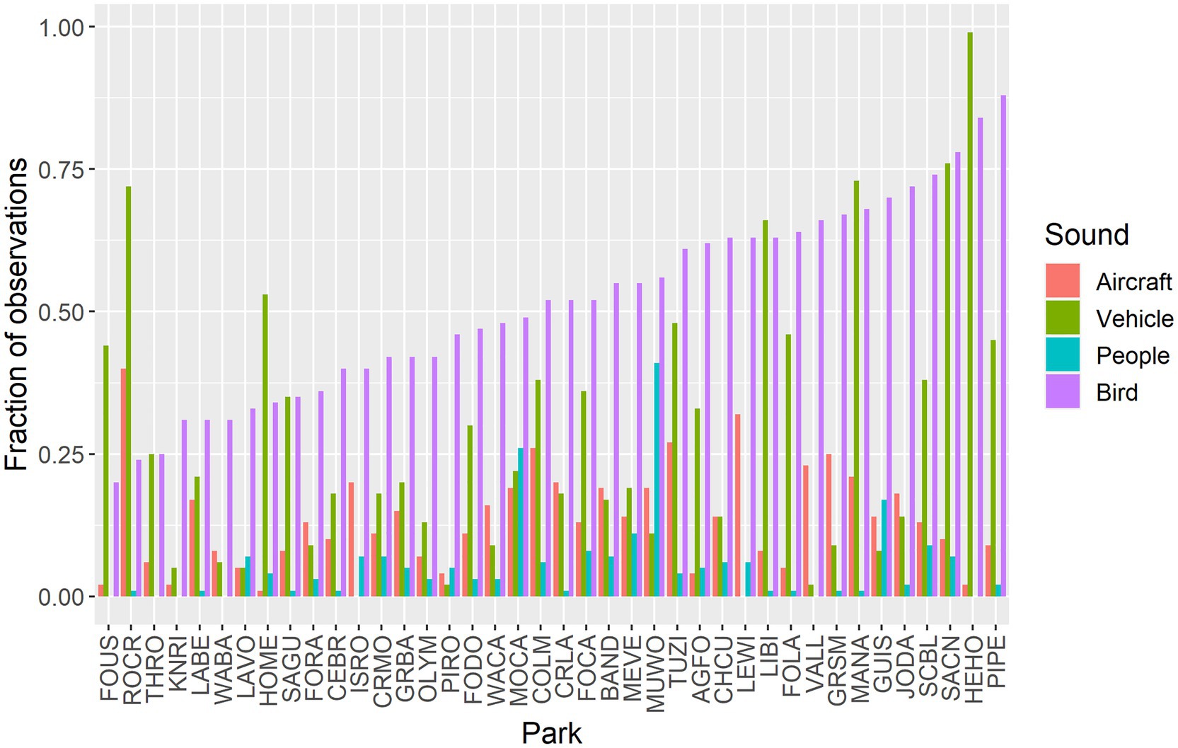
Figure 2. Fractions of observations with each sound, by park, ordered by bird detections.
Fitted model summary
Automated smooth term selection did not remove any noise terms from the proposed model explaining bird detection. The final model included smoothing spline functions for history of exposure to aircraft noise, history of exposure to vehicle noise, history of exposure to sounds from people, sun altitude, week of year, and a random effect term for site (Figure 3). The final model outperformed the null model with random effects (ΔAIC = 185,221.3) and fitted 29.2% of the null deviance. The model intercept, when transformed to a probability with the logistic function, was 0.168—indicating that the baseline probability of bird detection was estimated to be around 17%.
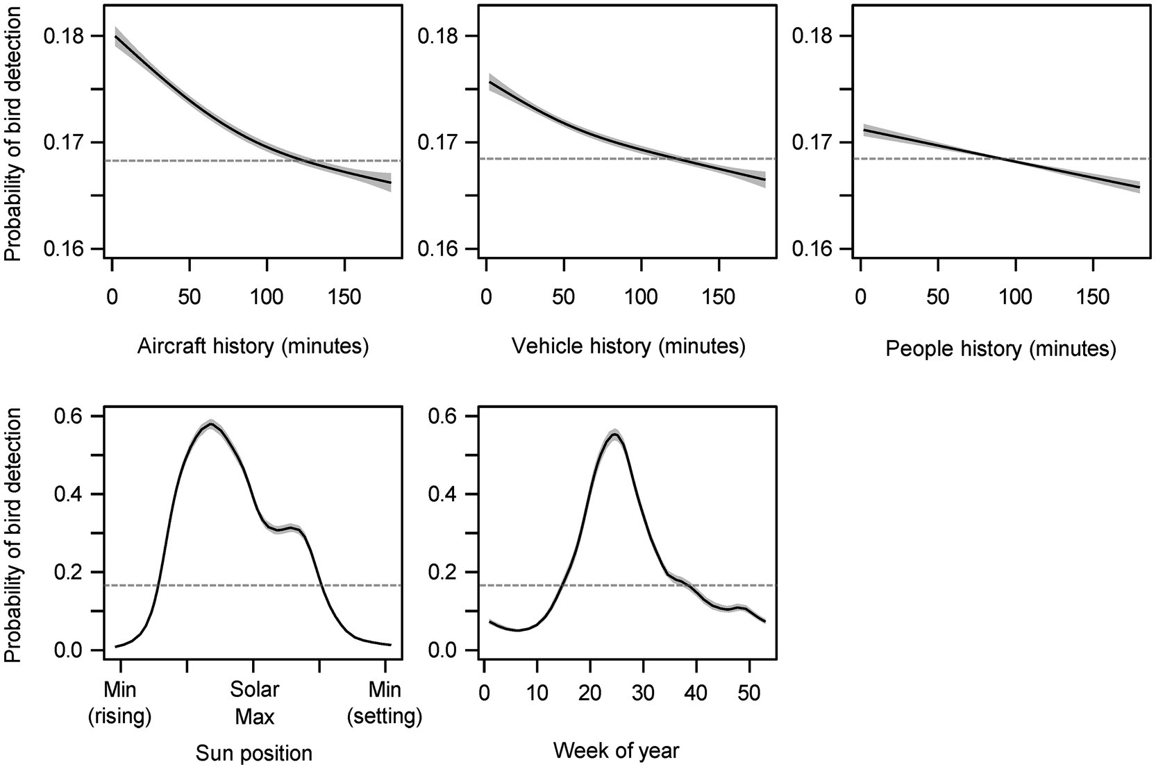
Figure 3. Partial effects plots for smoothed terms included in the general additive model. The gray shaded areas represent 95% confidence intervals. Each modeled effect has been transformed by the logistic function and shifted by the model intercept. The model intercept (0.168) is represented by the gray dashed horizontal line, and sections of the spline that are above or below this baseline indicates that the variable has a positive or negative impact, respectively, on bird detection probability at these values.
All three noise sources were associated with immediate increases in bird detections that declined and transitioned to decreased probabilities of bird detections between 90 and 120 min in the past (Figure 3). Noise events 3 h in the past were depressing bird detection probabilities. The ranges from greatest increase (2 min past) to greatest decrease (3 h past) were 1.4% (aircraft), 0.9% (vehicles), and 0.5% (people). The same ordering applied to the effective degrees of freedom of the splines (nonlinearity): edf = 3.3 (aircraft), 2.9 (vehicles), and 2.0 (people). All spline terms were highly significant (p < 0.001).
The cubic regression spline fit for sun position estimated that bird detection probability increased from a low of 0.8% during early morning to a high of 57.9% before the solar maximum (edf = 14.32, p < 0.001; Figure 3). The cyclic cubic regression spline fit for the effect of week of year estimated that bird detection was at a low of 5.0% during the sixth week of the year and increased to a high of 55.3% during the 24th week of the year (edf = 12.62, p < 0.001; Figure 3).
Diel and seasonal factors exerted far greater influence on bird sound detection than noise. Note that the model offset term for bird detection probability (16.8%) was much smaller than the proportion of data samples with bird sounds present (49.6%) because most of our data were collected during spring and summer when the seasonal term made a significant positive contribution.
Results for parks and BCRs
To explore the effect of aircraft noise exposure on bird sounds across the entire sample, we computed the change in predicted probabilities of bird sound between the actual record of aircraft noise events and a fictitious scenario with all aircraft noise removed (set to zero). The fictitious scenario had 1% lower bird detection rates overall (compared with an average bird detection value of 49.6%). Sites with higher aircraft traffic generally exhibited larger differences (Figure 4). Across all 648,900 samples, ‘no aircraft noise’ conditions led to a predicted decrease of bird detection probability in 52.91% of the samples, a predicted increase in 36.15% of samples, and no predicted effect (<0.0001% difference in predicted bird probability) in 10.94% of samples. Note than an increase occurred when aircraft events between 120 and 180 min in the past outweighed the effects of fewer, more recent aircraft events. The greatest predicted decrease of bird song detection probability under ‘no aircraft noise’ conditions was an average 11.75% decrease at Lewis and Clark National Historic Park (LEWI) a park site with high aircraft traffic and low vehicle traffic. The smallest predicted impact of ‘no aircraft noise’ conditions at a park unit was an average decrease of 0.42% at Homestead National Monument of America (HOME), which had low levels of aircraft traffic and high levels of vehicle traffic.
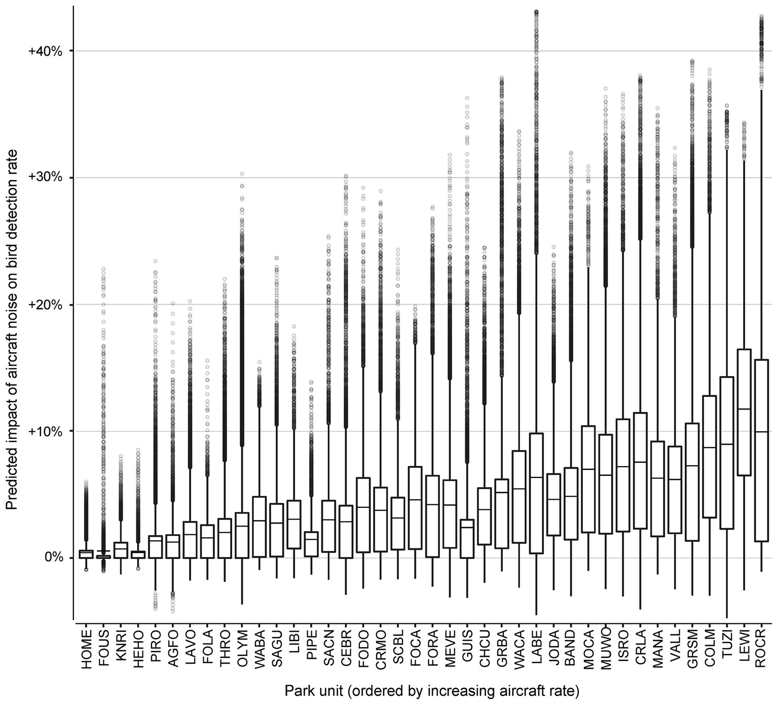
Figure 4. Projected influence of observed aircraft noise across 40 National Park units on bird detection probabilities relative to predicted rates under ‘no aircraft noise’ conditions. The park units have been ordered along the x-axis by increasing mean probability of aircraft detection. Points above 0 on the y-axis represent audio surveys that were predicted to have increased probability of bird detection under observed ‘aircraft noise’ conditions, while points below 0 on the y-axis represent audio surveys predicted to have decreased probability of bird detection under ‘aircraft noise’ conditions. The middle line is the mean difference in bird detection probability at each park unit. The lower hinge is the 25-percent quantile, and the upper hinge is the 75-percent quantile. The distance between the lower and upper hinges is the inter-quartile range (IQR). The whiskers mark the most discrepant observations that are within 1.5*IQR of the nearest hinge value. National Park unit abbreviations are Agate Fossil Beds National Monument (AGFO), Bandelier National Monument (BAND), Cedar Breaks National Monument (CEBR), Chaco Culture National Historical Park (CHCU), Colorado National Monument (COLM), Crater Lake National Park (CRLA), Craters of the Moon National Monument (CRMO), Fort Caroline National Memorial (FOCA), Fort Donelson National Battlefield (FODO), Fort Laramie National Historic Site (FOLA), Fort Raleigh National Historic Site (FORA), Fort Union Trading Post National Historic Site (FOUS), Great Basin National Park (GRBA), Great Smoky Mountains National Park (GRSM), Gulf Islands National Seashore (GUIS), Herbert Hoover National Historic Site (HEHO), Homestead National Monument of America (HOME), Isle Royale National Park (ISRO), John Day Fossil Beds National Monument (JODA), Knife River Indian Villages National Historic Site (KNRI), Lava Beds National Monument (LABE), Lassen Volcanic National Park (LAVO), Lewis and Clark National Historical Park (LEWI), Little Bighorn Battlefield National Monument (LIBI), Manassas National Battlefield Park (MANA), Mesa Verde National Park (MEVE), Montezuma Castle National Monument (MOCA), Muir Woods National Monument (MUWO), Olympic National Park (OLYM), Pipestone National Monument (PIPE), Pictured Rocks National Lakeshore (PIRO), Rock Creek Park (ROCR), Saint Croix/Lower St. Croix National Scenic River (SACN), Saguaro National Park (SAGU), Scotts Bluff National Monument (SCBL), Theodore Roosevelt National Park (THRO), Tuzigoot National Monument (TUZI), Valles Caldera National Preserve (VALL), Washita Battlefield National Historic Site (WABA), Walnut Canyon National Monument (WACA).
Automated smooth term selection for each of 19 subsets of data from BCRs excluded aircraft noise history from the top model for Boreal Hardwood Transition, Central Mixed Grass Prairie, and Eastern Tallgrass Prairie. Vehicle noise history was excluded from the Eastern Tallgrass Prairie, while the history of exposure to people was excluded from Northern Rockies, Prairie Hardwood Transition, and Sierra Nevada. Although the estimated size of the effect was variable, the general effect of aircraft exposure history on bird detection probability across BCRs resembled the shape of the spline estimated in the full model (Figure 5).
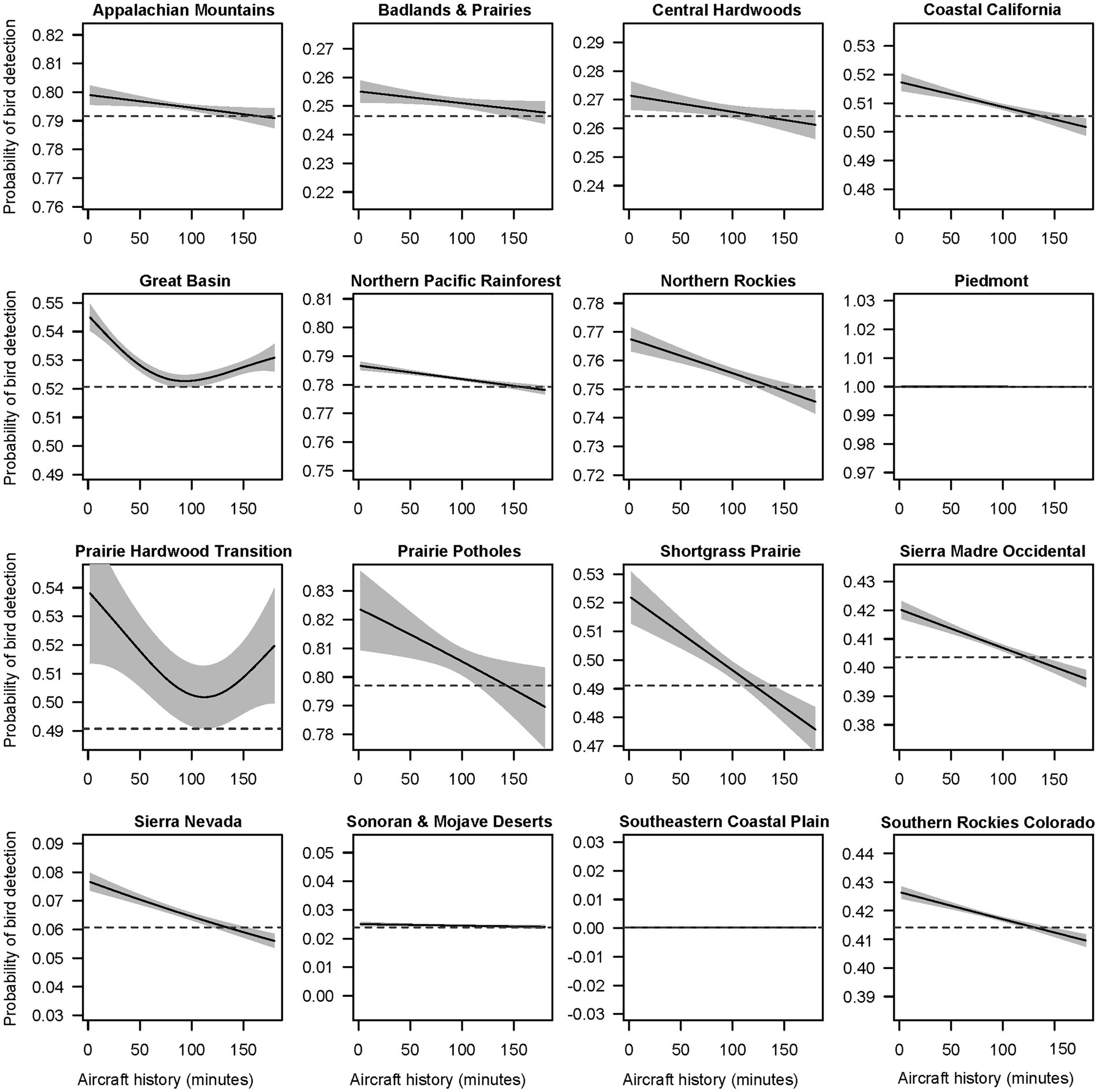
Figure 5. Smoothing spline functions for the effect of aircraft noise history on bird detection probabilities in Bird Conservation Regions (BCR). The panels were produced by fitting separate models to a subset of audio survey data from each BCR. Not all BCRs are represented above as aircraft noise was removed by model selection in Boreal Hardwood Transition, Central Mixed Grass Prairie, and Eastern Tallgrass Prairie.
Discussion
Aircraft noise effects and mitigation
Bird bioacoustic activity increased in the presence of all three noise sources and exhibited similar patterns of influence for past noise events. For aircraft noise, process(es) underlying this response likely involve auditory masking or distraction, and not responses to the visual stimulus of the noise source or the immediate threat the noise source might pose. We acknowledge that any unfamiliar noise could evoke a fearful response; but it is likely that habituation would extinguish a ‘fear of the unknown’ response given daily exposure to large numbers of aircraft for several decades. Though aircraft noise was not associated with the proximity of a probable threat, aircraft evoked the largest and longest lasting response. We note that the presence of noise in a 10 s sample inhibited our listeners’ capacity to detect bird sounds, so our model is likely underestimating the increase in bird sounds due to noise.
There is no precedent or provision for the Federal Aviation Administration (FAA) to manage high-altitude commercial jet traffic to reduce ecological or human impacts. The FAA categorically excludes aircraft operations above 10,000′ above ground level (AGL) from environmental impact analyses (FAA, 2004), though consideration will be given for aircraft noise analyses between 10,000′ and 18,000′ AGL over National Parks and Wildlife Refuges when the change is likely to be highly controversial (FAA, 2012b). Aircraft are the dominant contributors to noise across all National Park units (Buxton et al., 2019): every site had aircraft noise. Existing sound levels are more than double the predicted natural sound levels in 63% of all protected areas in the conterminous U.S. (Buxton et al., 2017). The NPS accepted the 18,000′ AGL criterion when they clarified their definition of “substantial restoration of natural quiet” at Grand Canyon National Park (NPS, 2008). At the times these policies were established, there was no evidence of adverse ecological effects from high altitude jet noise.
If ubiquitous commercial jet traffic presents ecological concerns, this study’s findings suggest a practical option for reducing impacts: concentrate traffic. The extended after-effects of a single aircraft event indicate that intervals between flights may need to be several hours to permit communities to return to baseline vocal rates. Conserving areas with very low aircraft traffic would be desirable. Also, it is possible that relatively constant noise conditions present a scenario that presents opportunities for learned or evolved adaptations to these conditions. A consolidation of aircraft traffic was implemented over Rocky Mountain National Park, as part of the revised area navigation procedures and optimized profile descent for Denver International Airport (FAA, 2012a). The Wild Basin and Mummy Range areas of the park became substantially quieter. Though it would be very difficult to contrive playback experiments that mimicked the spatio-temporal pattern of high-altitude aircraft noise, future redesigns of airspace utilization above 18,000′ or adjacent to airports offer opportunities to experimentally probe the patterns we found, by matching habitats that transition from quieter to louder and the converse, using habitats with unchanged exposures as controls.
Which species, what types of sounds?
A significant limitation of these data is ignorance about the breadth of species’ contributions to the observed pattern and what types of bird sounds were produced. A study in Denali National Park found that aircraft noise at the remote site caused an increase in the diversity of bird calls detected, indicating a broad community response (Vincelette et al., 2021). They and we speculate that increases in alarm and contact calls were responsible for much of the observed trend, but our data lack direct evidence on this point. However, indirect support for this interpretation comes from detections of mammalian sounds in our data. In parallel analyses, we found increased probabilities of detecting mammalian sounds during and after noise events, with very similar decays of the temporal weighting functions. Our Listening Lab coordinator’s experience with these data suggests that almost all of these mammalian sounds were sciurid alarm and contact calls. These species are prominent callers in response to predators and other perceived hazards, and they encode referential information about hazards in their calls (Greene and Meagher, 1998; Newar and Bowman, 2020).
Why would different noise sources evoke similar responses?
It was surprising that responses to these three noise sources were so similar. Human voices signified the proximity of people, which might scan as an immediate threat or disturbance for many birds and reduce foraging efficiency (Blumstein et al., 2005). Human voices could plausibly be a distracting stimulus, but voices would very rarely be so continuous as to cause significant auditory masking. In contrast, each aircraft presents a continuous masking effect for several minutes in locations with low ambient sound levels, yet this noise was not associated with a nearby, embodied threat. While some animals might plausibly react more strongly to noise whose source is not identifiable – due to elevated uncertainty about risk – such reactions would likely diminish after decades of exposure to many flights per day. The more likely explanation for this shared response is that proximal threats and reduced capacity to sense such threats both contribute to the landscape of fear (Laundré et al., 2010).
Birds routinely produce more alarm or alerting calls when humans are present. Yet why would noise masking increase bioacoustic activity? If silence is an important signal of predators in frogs and other species (Dapper et al., 2011), noise masking may result in a similar impression: absence of expected sounds. Indeed, many species likely eavesdrop on the ordinary, non-alarm signals of birds and other species to gain assurance of safety (Lilly et al., 2019). Perceptions of increased risk may increase production of socially contagious sounds, including vocal elicitations of social cooperation for predator surveillance (Uster and Zuberbüler, 2001). Increases in calling rates also may reflect compensatory efforts to restore functions of conspecific and interspecific communication networks (McGregor, 2005; Tobias et al., 2014). Why did aircraft noise evoke a stronger response? Though aircraft noise may be present greater risks to some birds, it also may be that the risks aircraft noise presents can be substantially reduced by eliciting more social calling (Uster and Zuberbüler, 2001). In the latter case, increases in bird bioacoustic activity might be due to heterogenous responses: calling in response to the proximal threat of humans (and possibly vehicles) and calling to elicit social mitigation of lost auditory awareness.
Note that compensatory increases in bird sound levels when noise was present (Brumm and Zollinger, 2011) cannot explain the pattern we observed, unless elevated sound levels persisted for long periods after the noise ended or the increases exceeded the amount needed to maintain a constant active space.
Extended duration of effects
Noise events that occurred tens of minutes in the past were associated with increased bioacoustic activity, and noise events up to 3 h in the past – the limit of our analysis – decreased bioacoustic activity with respect to expected levels. Plainly, the impacts of noise are not limited to the durations of the noise events. Several plausible mechanisms might contribute to the extended behavioral responses documented in this study. Stress responses require tens of minutes to resolve, and noises exhibit the unpredictability and uncontrollability that characterize stressors (Koolhaas et al., 2011). Field studies have shown that noise induces stress in breeding birds (Blickley et al., 2012; Kleist et al., 2018). If animals respond to proximal threats or decreased auditory awareness with increased production of contact or alarm calls, as supported by the results in this study, diverse mechanisms of individual and social equilibration could result in gradual relaxation back to undisturbed sound production patterns. In addition, auditory masking or distraction can plausibly inhibit the perception of auditory scenes (Marinato and Baldauf, 2019), especially the integration of subtle or infrequent acoustic cues. Lower signal-to-noise ratios also devalue the information encoded in alarm calls (Templeton and Greene, 2007). Accordingly, restoring the integrity of auditory surveillance – for individuals and communities of eavesdropping species – could be a slow process, possibly involving reacquisition of evidence regarding the reliability of nearby signalers (Marshall et al., 2017). The suppression of bioacoustics activity by noise experienced more than 100 min ago indicates that individuals and communities may experience a form of fatigue or refractory period after previously being stimulated by noise.
Does this subtle bioacoustic response signify substantive consequences?
Our analyses revealed a 1.2% increase in bird acoustic detections due to aircraft noise in the present moment; median increases due to aggregate noise exposures were approximately 10% at the most responsive sites. Viewed from the perspective of energetic budgets, these changes in vocalization effort have negligible consequences (Zollinger and Brumm, 2015). Yet this nuanced change in vocal activity may betoken significant changes in vigilance, mobility, and curtailed activity patterns. For roads (Fahrig and Rytwinski, 2009) and populated hiking paths (Blumstein et al., 2005; Bötsch et al., 2018), there is abundant evidence of reduced foraging success and populations densities in wide range of avian species. Absence of hikers from otherwise popular hiking trails due to COVID restrictions caused substantial increases in mammalian trail camera detections – including more daytime detections – for an assemblage of 24 species in Glacier National Park (Anderson et al., 2023). High-altitude aircraft noise evoked similar, but stronger, bioacoustic responses to road and human noise (and presence), suggesting that aircraft noise could cause similar ecological effects. Aircraft noise also might be more problematic than road or hiker noise because individuals cannot simply disperse to less disturbed habitats (Gill et al., 2001): all nearby areas would experience the same noise levels.
Transportation noise and people are sources of disturbance or diminished auditory awareness for many species throughout most of North America. This study showed that responses to transient noise or disturbance events may persist for a few hours – an interval that must be considered when measuring the cumulative effects of multiple events. This study also showed that high-altitude aircraft noise, vehicle noise, and sounds from people evoked similar responses, despite orders of magnitude differences in distances to the noise source. Jointly, these results indicate that the spatial and temporal extent of noise effects are much larger than the combined noise footprints of all sources might suggest. Individual high-altitude jets cruise at over 800 km per hour and project noise at least 40 km laterally. Each aircraft can have lingering effects of an uncertain magnitude on millions of hectares of habitat. Accordingly, it is important to identify the sound types, species, and biological processes underlying our results, to discern the extent of population consequences and conservation concerns that the subtle bioacoustic response portends.
Data availability statement
Publicly available datasets were analyzed in this study. This data can be found here: to be determined, pending discussions with the National Park Service.
Ethics statement
Ethical review and approval was not required for the animal study because the data were collected using passive, remote, audio recording instruments. No animals were captured, handled, or subject to close observation.
Author contributions
NK led the data analysis, with assistance from KF and RB. All authors contributed to the design of the study and writing the manuscript.
Funding
Funding was provided by the National Park Service through cooperative agreement numbers P14AC00728 and P17AC00971.
Acknowledgments
This study relied upon acoustic data collected by the Natural Sounds and Night Skies Division with assistance from NPS employees at the parks. The sound annotations were generated by a collective of NPS employees, Colorado State research assistants, and the undergraduates of the Colorado State Listening Lab.
Conflict of interest
The authors declare that the research was conducted in the absence of any commercial or financial relationships that could be construed as a potential conflict of interest.
Publisher’s note
All claims expressed in this article are solely those of the authors and do not necessarily represent those of their affiliated organizations, or those of the publisher, the editors and the reviewers. Any product that may be evaluated in this article, or claim that may be made by its manufacturer, is not guaranteed or endorsed by the publisher.
References
Anderson, A. K., Waller, J. S., and Thornton, D. H. (2023). Partial COVID-19 closure of a national park reveals negative influence of low-impact recreation on wildlife spatiotemporal ecology. Sci. Rep. 13:687. doi: 10.1038/s41598-023-27670-9
Aschoff, J. (1966). Circadian activity pattern with two peaks. Ecology 47, 657–662. doi: 10.2307/1933949
Bayne, E. M., Habib, L., and Boutin, S. (2008). Impacts of chronic anthropogenic noise from energy-sector activity on abundance of songbirds in the boreal Forest. Conserv. Biol. 22, 1186–1193. doi: 10.1111/j.1523-1739.2008.00973.x
Blickley, J. L., Word, K. R., Krakauer, A. H., Phillips, J. L., Sells, S. N., Taff, C. C., et al. (2012). Experimental chronic noise is related to elevated fecal corticosteroid metabolites in Lekking male greater sage-grouse (Centrocercus urophasianus). PLoS One 7:e50462. doi: 10.1371/journal.pone.0050462
Blumstein, D. T., Fernández-Juricic, E., Zollner, P. A., and Garity, S. C. (2005). Inter-specific variation in avian responses to human disturbance. J. Appl. Ecol. 42, 943–953. doi: 10.1111/j.1365-2664.2005.01071.x
Bötsch, Y., Tablado, Z., Scherl, D., Kéry, M., Graf, R. F., and Jenni, L. (2018). Effect of recreational trails on forest birds: human presence matters. Front. Ecol. Evol. 6. Available at:. doi: 10.3389/fevo.2018.00175
Brumm, H., and Slater, P. J. B. (2006). Ambient noise, motor fatigue, and serial redundancy in chaffinch song. Behav. Ecol. Sociobiol. 60, 475–481. doi: 10.1007/s00265-006-0188-y
Brumm, H., and Zollinger, S. A. (2011). The evolution of the Lombard effect: 100 years of psychoacoustic research. Behaviour 148, 1173–1198. doi: 10.1163/000579511X605759
Buxton, R. T., McKenna, M. F., Mennitt, D., Brown, E., Fristrup, K., Crooks, K. R., et al. (2019). Anthropogenic noise in US national parks–sources and spatial extent. Front. Ecol. Environ. 17, 559–564. doi: 10.1002/fee.2112
Buxton, R. T., McKenna, M. F., Mennitt, D., Fristrup, K., Crooks, K., Angeloni, L., et al. (2017). Noise pollution is pervasive in U.S. protected areas. Science 356, 531–533. doi: 10.1126/science.aah4783
Dapper, A. L., Baugh, A. T., and Ryan, M. J. (2011). The sounds of silence as an alarm cue in Túngara frogs, Physalaemus pustulosus. Biotropica 43, 380–385. doi: 10.1111/j.1744-7429.2010.00707.x
FAA (2004). 1050.1E - environmental impacts: Policies and procedures. Available at: https://www.faa.gov/regulations_policies/orders_notices/index.cfm/go/document.information/documentID/13975 (Accessed January 15, 2023).
FAA (2012a). 2012 final FAA RNAV and RNP procedures at Denver international airport and Rocky Mountain metropolitan airport environmental assessment and finding for no significant impact (FONSI) and record of decision (ROD). Available at: https://www.faa.gov/air_traffic/environmental_issues/ared_documentation/media/FIN_RNAV_RNP_EA_28Aug_2012-29DenverIntlCentennialRockyMtnMetroAirport_FONSI_ROD.pdf (Accessed December 19, 2022).
Fahrig, L., and Rytwinski, T. (2009). Effects of roads on animal abundance: an empirical review and synthesis. Ecol. Soc. 14. doi: 10.5751/ES-02815-140121
Francis, C. D., Ortega, C. P., and Cruz, A. (2009). Noise pollution changes avian communities and species interactions. Curr. Biol. 19, 1415–1419. doi: 10.1016/j.cub.2009.06.052
Fristrup, K. M., Hatch, L. T., and Clark, C. W. (2003). Variation in humpback whale (Megaptera novaeangliae) song length in relation to low-frequency sound broadcasts. J. Acoust. Soc. Am. 113, 3411–3424. doi: 10.1121/1.1573637
Gill, J. A., Norris, K., and Sutherland, W. J. (2001). Why behavioural responses may not reflect the population consequences of human disturbance. Biol. Conserv. 97, 265–268. doi: 10.1016/S0006-3207(00)00002-1
Goudie, R. I., and Jones, I. L. (2004). Dose-response relationships of harlequin duck behaviour to noise from low-level military jet over-flights in Central Labrador. Environ. Conserv. 31, 289–298. doi: 10.1017/S0376892904001651
Greene, E., and Meagher, T. (1998). Red squirrels, Tamiasciurus hudsonicus, produce predator-class specific alarm calls. Anim. Behav. 55, 511–518. doi: 10.1006/anbe.1997.0620
Grolemund, G., and Wickham, H. (2011). Dates and times made easy with lubridate. J. Stat. Softw. 40, 1–25. doi: 10.18637/jss.v040.i03
Habib, L., Bayne, E. M., and Boutin, S. (2007). Chronic industrial noise affects pairing success and age structure of ovenbirds Seiurus aurocapilla. J. Appl. Ecol. 44, 176–184. doi: 10.1111/j.1365-2664.2006.01234.x
Herman, J. P., McKlveen, J. M., Ghosal, S., Kopp, B., Wulsin, A., Makinson, R., et al. (2016). Regulation of the hypothalamic-pituitary-adrenocortical stress response. Compr. Physiol. 6, 603–621. doi: 10.1002/cphy.c150015
Kaiser, K., and Hammers, J. (2009). The effect of anthropogenic noise on male advertisement call rate in the neotropical treefrog, Dendropsophus triangulum. Behaviour 146, 1053–1069. doi: 10.1163/156853909X404457
Kleist, N. J., Guralnick, R. P., Cruz, A., Lowry, C. A., and Francis, C. D. (2018). Chronic anthropogenic noise disrupts glucocorticoid signaling and has multiple effects on fitness in an avian community. Proc. Natl. Acad. Sci. U. S. A. 115, E648–E657. doi: 10.1073/pnas.1709200115
Koolhaas, J. M., Bartolomucci, A., Buwalda, B., de Boer, S. F., Flügge, G., Korte, S. M., et al. (2011). Stress revisited: a critical evaluation of the stress concept. Neurosci. Biobehav. Rev. 35, 1291–1301. doi: 10.1016/j.neubiorev.2011.02.003
Laundré, J. W., Hernández, L., and Ripple, W. J. (2010). The landscape of fear: ecological implications of being afraid. Open Ecol. J. 3, 1–7. doi: 10.2174/1874213001003030001
Lilly, M. V., Lucore, E. C., and Tarvin, K. A. (2019). Eavesdropping grey squirrels infer safety from bird chatter. PLoS One 14:e0221279. doi: 10.1371/journal.pone.0221279
Lynch, E., Joyce, D., and Fristrup, K. (2011). An assessment of noise audibility and sound levels in U.S. National Parks. Landsc. Ecol. 26, 1297–1309. doi: 10.1007/s10980-011-9643-x
Marinato, G., and Baldauf, D. (2019). Object-based attention in complex, naturalistic auditory streams. Sci. Rep. 9:2854. doi: 10.1038/s41598-019-39166-6
Marra, G., and Wood, S. N. (2011). Practical variable selection for generalized additive models. Comput. Stat. Data Anal. 55, 2372–2387. doi: 10.1016/j.csda.2011.02.004
Marshall, J. A. R., Brown, G., and Radford, A. N. (2017). Individual confidence-weighting and group decision-making. Trends Ecol. Evol. 32, 636–645. doi: 10.1016/j.tree.2017.06.004
McClure, C. J. W., Ware, H. E., Carlisle, J. D., and Barber, J. R. (2017). Noise from a phantom road experiment alters the age structure of a community of migrating birds. Anim. Conserv. 20, 164–172. doi: 10.1111/acv.12302
McClure, C. J. W., Ware, H. E., Carlisle, J., Kaltenecker, G., and Barber, J. R. (2013). An experimental investigation into the effects of traffic noise on distributions of birds: avoiding the phantom road. Proc. R. Soc. B Biol. Sci. 280:20132290. doi: 10.1098/rspb.2013.2290
Mennitt, D., Sherrill, K., and Fristrup, K. (2014). A geospatial model of ambient sound pressure levels in the contiguous United States. J. Acoust. Soc. Am. 135, 2746–2764. doi: 10.1121/1.4870481
NABCI (2014). NABCI bird conservation regions | birds Canada | Oiseaux Canada. Available at: https://www.birdscanada.org/bird-science/nabci-bird-conservation-regions ().
Newar, S. L., and Bowman, J. (2020). Think before they squeak: vocalizations of the squirrel family. Front. Ecol. Evol. 8. doi: 10.3389/fevo.2020.00193
NPS (2008). Public notice: clarifying the definition of “substantial restoration of natural quiet” at grand canyon National Park, AZ. Available at: https://www.federalregister.gov/documents/2008/09/24/E8-22343/public-notice-clarifying-the-definition-of-substantial-restoration-of-natural-quiet-at-grand-canyon (Accessed December 20, 2022).
NSNSD (2013). Acoustical monitoring training manual. Available at: https://www.nps.gov/subjects/sound/upload/NSNSDTrainingManual_AcousticalAmbientMonitoring-508.pdf (Accessed December 16, 2022).
Pedersen, E. J., Miller, D. L., Simpson, G. L., and Ross, N. (2019). Hierarchical generalized additive models in ecology: an introduction with mgcv. PeerJ 7:e6876. doi: 10.7717/peerj.6876
Senzaki, M., Barber, J. R., Phillips, J. N., Carter, N. H., Cooper, C. B., Ditmer, M. A., et al. (2020). Sensory pollutants alter bird phenology and fitness across a continent. Nature 587, 605–609. doi: 10.1038/s41586-020-2903-7
Slabbekoorn, H., and Peet, M. (2003). Birds sing at a higher pitch in urban noise. Nature 424:267. doi: 10.1038/424267a
Sun, J. W. C., and Narins, P. M. (2005). Anthropogenic sounds differentially affect amphibian call rate. Biol. Conserv. 121, 419–427. doi: 10.1016/j.biocon.2004.05.017
Templeton, C. N., and Greene, E. (2007). Nuthatches eavesdrop on variations in heterospecific chickadee mobbing alarm calls. PNAS 104, 5479–5482. doi: 10.1073/pnas.0605183104
Thieurmel, B. (2022). suncalc. Available at: https://github.com/datastorm-open/suncalc (Accessed December 18, 2022).
Tobias, J. A., Planqué, R., Cram, D. L., and Seddon, N. (2014). Species interactions and the structure of complex communication networks. Proc. Natl. Acad. Sci. 111, 1020–1025. doi: 10.1073/pnas.1314337111
Tyack, P. L., Zimmer, W. M. X., Moretti, D., Southall, B. L., Claridge, D. E., Durban, J. W., et al. (2011). Beaked whales respond to simulated and actual navy sonar. PLoS One 6:e17009. doi: 10.1371/journal.pone.0017009
Uster, D., and Zuberbüler, K. (2001). The functional significance of Diana monkey “clear” calls. Behaviour 138:741.
Van Rij, J., Wieling, M., Baayen, R. H., and van Rijn, D. (2015). Itsadug: Interpreting time series and autocorrelated data using GAMMs.
Vincelette, H., Buxton, R., Kleist, N., McKenna, M. F., Betchkal, D., and Wittemyer, G. (2021). Insights on the effect of aircraft traffic on avian vocal activity. Ibis 163, 353–365. doi: 10.1111/ibi.12885
Watkins, W. A., and Schevill, W. E. (1975). Sperm whales (Physeter catodon) react to pingers. Deep-Sea Res. Oceanogr. Abstr. 22, 123–129. doi: 10.1016/0011-7471(75)90052-2
Wilson, A. A., Ditmer, M. A., Barber, J. R., Carter, N. H., Miller, E. T., Tyrrell, L. P., et al. (2021). Artificial night light and anthropogenic noise interact to influence bird abundance over a continental scale. Glob. Chang. Biol. 27, 3987–4004. doi: 10.1111/gcb.15663
Wood, S. N. (2017). Generalized additive models: An introduction with R. 2nd New York: Chapman and Hall/CRC
Wood, S. (2021). Mgcv: mixed GAM computation vehicle with automatic smoothness estimation. Available at: https://CRAN.R-project.org/package=mgcv (Accessed March 21, 2021).
Keywords: anthropogenic, noise, bioacoustics, behavior, sensory ecology, cumulative impact
Citation: Kleist NJ, Fristrup KM, Buxton RT, McKenna MF, Job JR, Angeloni LM, Crooks K and Wittemyer G and (2023) Anthropogenic noise events perturb acoustic communication networks. Front. Ecol. Evol. 11:1149097. doi: 10.3389/fevo.2023.1149097
Edited by:
David Andrew Luther, George Mason University, United StatesReviewed by:
Felipe N. Moreno-Gómez, Universidad Católica del Maule, ChileMegan Gall, Vassar College, United States
Copyright © 2023 Kleist, Fristrup, Buxton, McKenna, Job, Angeloni, Crooks and Wittemyer. This is an open-access article distributed under the terms of the Creative Commons Attribution License (CC BY). The use, distribution or reproduction in other forums is permitted, provided the original author(s) and the copyright owner(s) are credited and that the original publication in this journal is cited, in accordance with accepted academic practice. No use, distribution or reproduction is permitted which does not comply with these terms.
*Correspondence: Nathan J. Kleist, nathan.kleist@gmail.com