
94% of researchers rate our articles as excellent or good
Learn more about the work of our research integrity team to safeguard the quality of each article we publish.
Find out more
ORIGINAL RESEARCH article
Front. Ecol. Evol., 09 March 2023
Sec. Population, Community, and Ecosystem Dynamics
Volume 11 - 2023 | https://doi.org/10.3389/fevo.2023.1146850
This article is part of the Research TopicThe Impacts of Climate Change and Human Activities on the Structure and Function of Wetland/Grassland EcosystemsView all 18 articles
 Wenjun Liu1
 Cong Xu2
 Zhiming Zhang1
 Hans De Boeck1,3
 Yanfen Wang4,5Liankai Zhang6,7Xiongwei Xu6,7Chen Zhang6,7Guiren Chen6,7Can Xu6,7*
The demand for accurate estimation of aboveground biomass (AGB) at high spatial resolution is increasing in grassland-related research and management, especially for those regions with complex topography and fragmented landscapes, where grass and shrub are interspersed. In this study, based on 519 field AGB observations, integrating Synthetic Aperture Radar (SAR; Sentinel-1) and high-resolution (Sentinel-2) remote sensing images, environmental and topographical data, we estimated the AGB of mountain grassland in Southwest China (Yunnan Province and Guizhou Province) by using remote sensing algorithms ranging from traditional regression to cutting edge machine learning (ML) and deep learning (DL) models. Four models (i.e., multiple stepwise regression (MSR), random forest (RF), support vector machine (SVM) and convolutional neural network (CNN)) were developed and compared for AGB simulation purposes. The results indicated that the RF model performed the best among the four models (testing dataset: decision co-efficient (R2) was 0.80 for shrubland and 0.75 for grassland, respectively). Among all input variables in the RF model, the vegetation indices played the most important role in grassland AGB estimation, with 6 vegetation indices (EVI, EVI2, NDVI, NIRv, MSR and DVI) in the top 10 of input variables. For shrubland, however, topographical factors (elevation, 12.7% IncMSE (increase in mean squared error)) and SAR data (VH band, 11.3% IncMSE) were the variables which contributed the most in the AGB estimation model. By comparing the input variables to the RF model, we found that integrating SAR data has the potential to improve grassland AGB estimation, especially for shrubland (26.7% improvement in the estimation of shrubland AGB). Regional grassland AGB estimation showed a lower mean AGB in Yunnan Province (443.6 g/m2) than that in Guizhou Province (687.6 g/m2) in 2021. Moreover, the correlation between five consecutive years (2018–2022) of AGB data and climatic factors calculated by partial correlation analysis showed that regional AGB was positively related with mean annual precipitation in more than 70% of the grassland and 60% of the shrubland area, respectively. Also, we found a positive relationship with mean annual temperature in 62.8% of the grassland and 55.6% of the shrubland area, respectively. This study demonstrated that integrating SAR into grassland AGB estimation led to a remote sensing estimation model that greatly improved the accuracy of modeled mountain grassland AGB in southwest China, where the grassland consists of a complex mix of grass and shrubs.
Grassland is one of the most widely distributed terrestrial ecosystems, accounting for more than 40% of the world’s land surface (Scurlock and Hall, 2002). It plays an important role in providing human livelihood through the livestock production of grazing animals and additional ecosystem services such as regulating the terrestrial carbon cycling, maintaining biodiversity and preventing soil erosion (Flombaum and Sala, 2007; Wang et al., 2010; Niu et al., 2014; Mu et al., 2016). Grassland aboveground biomass (AGB) is one of the key indicators for evaluating in grassland growth status, utilization, and related environment assessment (Ali et al., 2016). Therefore, the accurate and timely estimation of grassland AGB is crucial for research and optimizing management.
Traditional surveys of grassland AGB is directly measured by harvesting the aboveground materials, drying, and weighing in laboratories, which has high estimation accuracy but is limited to small areas due to its time-consuming nature and the labor involved (Sinha et al., 2015). With continuous launches of advanced satellites, leading to images with various spatial extent and temporal scales, coupled with the development of computing technology, remote sensing has become an efficient and low-cost approach which is widely applied in grassland monitoring at regional levels or global scales (Jin et al., 2014; Quan et al., 2017; Yang et al., 2018). The main principle of remote sensing based AGB estimation is to model the relationship between remote sensing parameters and field AGB observations, and subsequently apply the model to extrapolate AGB estimates to a regional scale. More specifically, there are three main categories of remote sensing-based grassland AGB estimation models or methods: empirical relationships with VIs, machine learning (ML) models and process-based model.
Establishing relationships between VIs and recorded AGB is the most common and direct approach for regional grassland AGB assessment. Many studies have reported that there is a strong correlation between the VIs, including normalized difference vegetation index (NDVI; Wei et al., 2021), enhanced vegetation index (EVI; Ge et al., 2018), soil adjusted vegetation index (SAVI; Ren et al., 2018), ratio vegetation index (RVI; Guerschman et al., 2009) and biomass in varies satellite images. However, VIs are subjected to the influence of environmental condition and the capability of characterizing vegetation status in certain circumstance, which can introduce errors and uncertainties into AGB estimation (Ali et al., 2016). In recent years, efforts have been made to improve the estimation accuracy by constructing estimation model with multiple VIs or introducing specific VIs transformation to enhance the sensitivity of VIs to AGB or decrease the influences by environmental factors such as soil and other background factors (Li et al., 2013, 2016). ML methods, the non-parametric models constructed by both remote sensing images and environment data, are to find solutions that optimize performance metrics for a certain parameter from multiple sources based on a “learning process” (Jordan and Mitchell, 2015). These methods can integrate multiple factors, learn from complicated nonlinear data, and provide better simulations than empirical regression models (Powell et al., 2010). Moreover, ML models could provide accurate estimations of nonlinear relationship from various data, which help increase understanding of the driving forces in the ecosystem research (Ramoelo et al., 2015). Over the last decades, AGB assessment methods have been developed ranging from traditional multiple linear regression (MLR) to ML models such as support vector machine (SVM), random forests (RF) and artificial neural network (ANN). Nowadays, ML models have been widely applied in remote sensing grassland AGB estimation (Morais et al., 2021). A recent literature review on ML methods used for grassland AGB estimation pointed out that the RF model was the most frequently used algorithm, followed by partial least squares regression (PLSR), but there was no significant difference between the accuracy of ML models (Morais et al., 2021). Various conclusions have been reported in ML model comparison studies, for examples, Zeng et al. (2019, 2021) used four ML model in grassland AGB simulations and found that the RF model performed the best, explaining 86% of the observed data variation on the Tibetan Plateau, while Zhang et al. (2018) reported ANN was better in a sawgrass marsh AGB prediction. In addition, considering there is no evidence that the performance of the ML algorithms themselves has been improving over time, and since the training process and the equations of the ML models cannot be observed, the applicability of ML models still needs to be analyzed to select suitable models in specific studies (Ali et al., 2016; Yang et al., 2018). Besides the above mentioned classical ML models, the use of deep learning, an advanced ML technique which can automatically extract high dimensional ‘hidden’ features through a deeper neural network with hierarchical structure, has increased in recent years (LeCun et al., 2015). Convolutional neural network (CNN) is considered as the most representative among them, which has been widely used in image classification (Wang et al., 2021). CNN model usually includes input layer, convolutional layer, pooling layer, fully connected layer and output layer. Unlike image classification, the last layer of CNN model for regression prediction accumulates the previous layer directly without adding soft-max function. However, AGB estimation usually lacks enough samples for CNN model training, and thus the potential of using CNN for AGB estimation is not well established yet (Dong et al., 2020).
Besides the ML algorithms selection, input variables are another relevant factor affecting grassland AGB estimation accuracy. Independent variables (or explanatory variables) such as meteorological, topographical, and geographic variables are the most common environmental variables, while the abundance of VIs provided by optical remote sensors are the main remote sensing input parameters. However, the use of optical data for estimating grassland AGB has several limitations including that the acquisition of high quality images is restricted by weather conditions, spectral information and VIs saturation occurring in dense vegetation areas, while it also lacks the ability to provide vegetation structure information (Lu, 2007). Synthetic aperture radar (SAR) sensors can penetrate through clouds without illumination conditions limitations, and the SAR system can provide valuable information about vegetation structure though a series of algorithms (Barrett et al., 2014). Therefore, integration of optical and SAR data could overcome several limitations and thus could improve the performance of grassland AGB estimations (Naidoo et al., 2019). The potential of this integration has been proven in a grazed grassland (Wang et al., 2019), and thus it is worth to apply the concept in a more complex vegetation, such as shrubby grassland.
Located at the intersection of South and East Asia, the Yunnan-Guizhou plateau including Yunnan and Guizhou provinces is the dominant feature of Southwest China. Influenced by South and East Asian Monsoons and complex topography, the vegetation of Yunnan-Guizhou plateau is highly varied, ranging from subtropical forest to open grasslands (Chu et al., 2021). The plateau is the main distribution area of China’s thermal shrub grassland, which consists of patches of grass hills, grass slopes, scrub grassland, dry savanna, and alpine meadows, which all are relevant for developing animal husbandry (Shen et al., 2016). However, grassland ecosystems in Southwest China are relatively understudied in the earth observation field. There is still a knowledge gap with respect to the estimation of regional aboveground biomass for grassland with complex topography and high small-scale heterogeneity.
In this study, our primary objectives were to (1) develop and compare the capability of four models including a traditional regression model [i.e., multiple stepwise regression (MSR)], two classical ML models (i.e., RF, SVM) and a deep learning model (i.e., CNN) in grassland AGB estimation in Southwest China. (2) explore the potential of integrating SAR (Sentinel-1) and high resolution optical remote sensing (Sentinel-2) with gridded environmental and topographic data to develop regional grassland AGB estimation model to derive the spatial patterns of AGB for the Southwest China grassland of 2021, and (3) analyze the spatial and temporal variation of grassland AGB in Southwest China and its response to climatic factors, by mapping the grassland AGB from 2018 to 2022.
The study area includes Yunnan and Guizhou provinces (21°8′–29°15′N, 97°31′–109°35′E), in which the Yunnan-Guizhou plateau is located (Figure 1). These two provinces cover about 570,000 km2 with a large elevational span, ranging from less than 100 m to over 6,000 m a.s.l., with much of the region being mountainous or dotted with karst landscapes. The climate belongs to highland monsoon climate, with small annual but large daily temperature differences, and abundant radiation and rainfall. The mean annual temperature in the study area is 24°C, and the mean annual precipitation is approximately 1,100 mm, with around 80% concentrated in summer and autumn based on the data from 22 meteorological stations over the past 20 years. A highly variable climate and edaphic space provides suitable light, soil and climate for diverse vegetation development and creates a rich diversity of biological resources. Grassland and shrubland are important vegetation types in the region accounting for over 14% of the area, with about 40% of Southern China’s grassland area is located in Yunnan based on data derived from a national grassland survey (Wu et al., 2017). The mainly grassland types include alpine meadows, temperate grassland, and mountain grassland, while warm shrubland, dry and hot sparse tree shrubland and thermal shrubland are the main shrubland types. Grassland and shrubland are distributed over almost the entire area except for the southwestern part of the study area, but the complex topographic conditions of the area determine the fragmented distribution of grassland and shrubland.
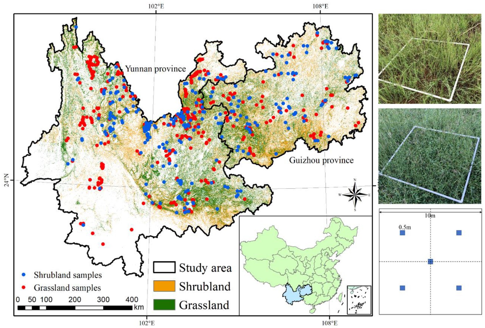
Figure 1. The location of the study area and the distribution of shrubland and grassland, as well as field data sample points.
Field data surveys were conducted during the growing season of 2021. In order to match the ground samples with the satellite data, we regularly set five sample plots of 1 m × 1 m at each sample points for grassland and set one sample plots of 5 m × 5 m for shrubland with an interval distance of over 1 km between the plots so as to assure the representativeness of the samples. AGB of grassland and shrubland were acquired by harvesting all aboveground portions of vegetation within the sample plots, and weighing dried biomass. Moreover, the geographic coordinate pairs of each sample plot were also accurately recorded by a Trimble GeoXH 3,000 handheld GPS with decimeter-level position accuracy for acquiring the corresponding features of satellite data. A total of 519 samples including 298 samples for pure grassland and 221 samples for shrubland were collected across the study area, covering cover all the typical types of the grassland and shrubland (Figure 1).
Sentinel-2 (S2) images covering the study area were acquired and processed through Google Earth Engine (https://code.earthengine.google.com/, GEE). In order to maintain consistency with ground measured data, all available imageries of S2A in the July and August, 2021 were collected, as well as supplemental images in May, June, September, and October whenever the region was not covered by clouds. Sentinel-2 covers 13 spectral bands from visible and near-infrared to short-wave infrared with a revisit period of 5 days and a spatial resolution from 10 to 60 m. It also contains three bands in the red-edge range, which is effective for monitoring vegetation information. We obtained the reflectance of 11 raw bands and calculated 11 vegetation indices based on the 11 bands as the input variables.
Sentinel-1 (S1) consists of two satellites, A and B, carrying a C-band synthetic aperture radar (SAR) that provides continuous imagery during day, night, and all types of weather. The polarization mode of S1 includes the single polarization mode (HH or VV) and the dual polarization mode (HH + HV or VV + VH). VH and VV are commonly used for the estimation of vertical parameters. Moreover, to match with the data from field measurements, we used data of S1 with 10 m spatial resolution in early August for AGB estimation.
Topography factors were obtained from digital elevation model (DEM) data with 12.5 m spatial resolution, which is the elevation data collected by ALOS (Advanced Land Observing Satellite) phased array type L-band synthetic aperture radar (PALSAR). ALOS DEM elevation data has a horizontal and vertical accuracy of 12.5 m, which can be downloaded on https://search.asf.alaska.edu/. Based on the elevation data, slope and aspect were calculated for each pixel.
Environmental data was collected from three sources: the derived products of MODIS (MOD11A2.006) provides the terra land surface temperature with 1 km spatial resolution; A downscaled precipitation product with 1 km spatial resolution developed by Elnashar et al. (2020) was used to extract the annual mean precipitation; Water Vapor Pressure (Water VP) was from S2.
Landcover types data was obtained from the latest ChinaCover dataset with 10 m spatial resolution (provided by the State Key Laboratory of Remote Sensing Science, Aerospace Information Research Institute, Chinese Academy of Sciences, China. The data was updated in 2020, but not released yet; Wu et al., 2017), from which we extracted the grassland and shrubland to represent the great definition of grassland in this study.
Five types of features were used as input variables for machine learning models for the estimation of shrubland and grassland AGB (Table 1), including remote sensing spectral bands (Blue, Green, Red, Edge 1, Edge 2, Edge 3, Near Infrared (NIR), Edge 4, Water vapor, short-wave infrared 1 (SWIR 1) and SWIR 2) and VIs calculated by spectral bands (SR, NDVI, MSR, DVI, SAVI, EVI, NIRv, kNDVI, EVI2, GCC, and Clred Edge) from Sentinel-2, C-band SAR (VV and VH) from Sentinel-1; three topography factors (elevation, aspect and slope) from ALOS, and three environmental factors [Water VP, annual mean precipitation (Precipitation) and land surface temperature (LST)] from MODIS and downscaling algorithms. All the features corresponding to each sample points were extracted and then used in the model training and validation combined with ground measured AGB of grassland and shrubland.
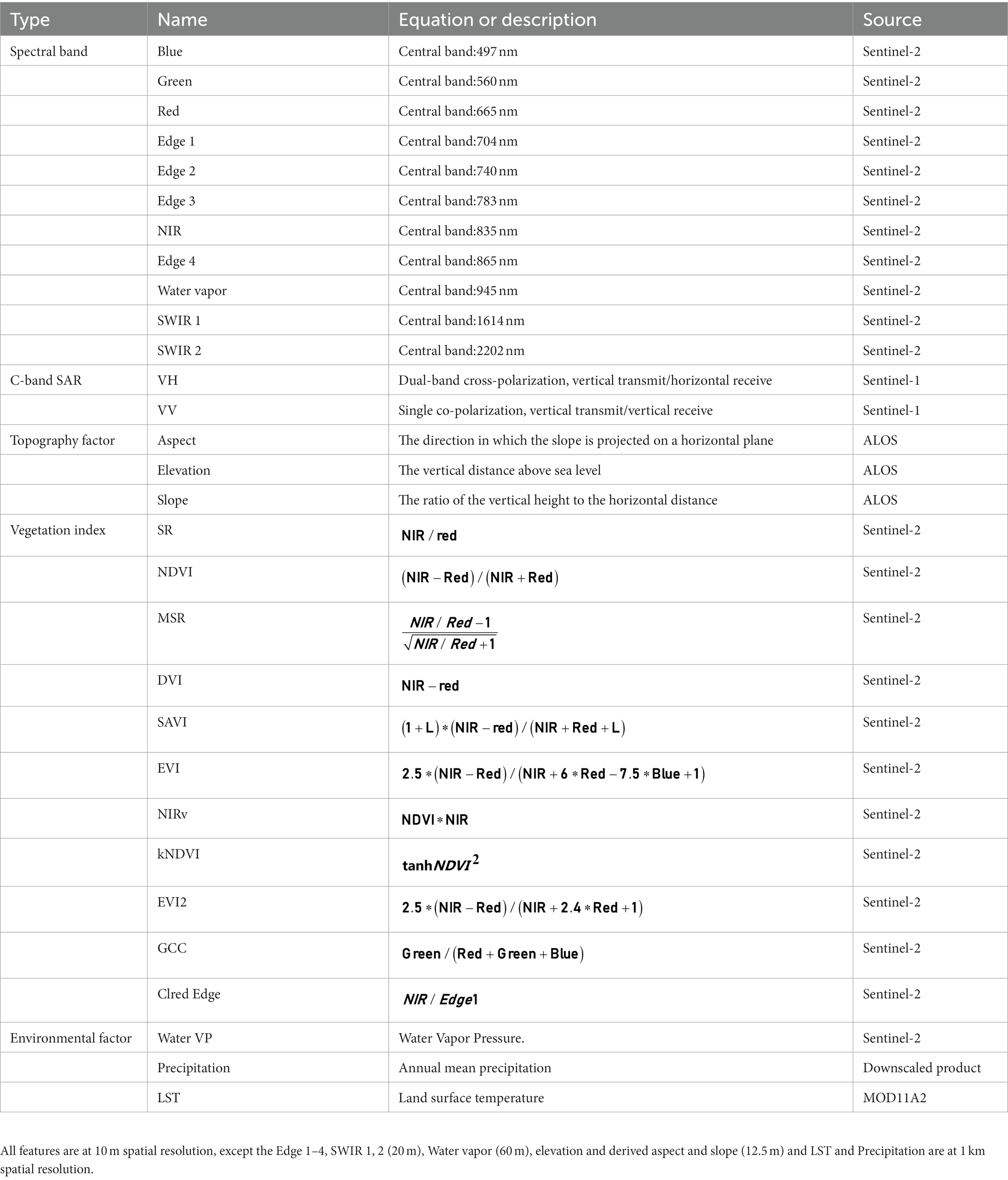
Table 1. Features from remote sensing data as inputs of machine learning models for aboveground biomass estimation of grassland and shrubland.
Four models for predicting the aboveground biomass are used in our study: multiple stepwise regression (MSR), random forest (RF), support vector machine (SVM), and convolutional neural network (CNN).
MSR is a statistical analysis method used to determine the quantitative relationship of interdependence between two or more variables. It understands and interprets the relationships between AGB and the features from satellite data intuitively, and is sensitive to the abnormal values as well (Wu et al., 2016).
RF is a compositional supervised learning method that can be considered as an extension of decision trees. The RF regression model builds multiple unrelated decision trees by randomly drawing the input features to obtain prediction in a parallel manner. It is the most-used method for grassland AGB prediction (Wang et al., 2019; Zeng et al., 2019). Each decision tree yields a prediction result from the extracted samples and features, and the regression prediction result of the whole forest is obtained by combining the results of all trees and taking the average, to reduce the risk of overfitting. A Bayesian optimization procedure is applied to determine the number of trees and the number of selected predictors for each tree.
SVM maps input features to a high-dimensional space through functions and uses kernel functions to effectively overcome the dimensional catastrophe caused by mapping. It is based on the principle of finding a regression plane such that all the data of a set are closest to that plane. The method is suitable for small-sample, nonlinear prediction problems and has good generalization ability (Zhang et al., 2015).
CNN is a deep learning method that deduces features of the next layer by using convolution kernel with shared weights, which greatly reduces the number of parameters that need to be trained. Based on the AGB of samples and their corresponding remote sensing features, we built a simplified CNN model and added a one-dimensional convolution layer. The input shape was defined by our independent variables. We added flatten and dense layers and optimized them using the Adam algorithm. ReLU (Krizhevsky et al., 2017) and root mean square error (RMSE) were used as the activation and function.
The workflow to establish the best AGB estimation model in this study is shown in Figure 2. Specifically, firstly, considering grassland is a mix grassy vegetation and shrubs in the study area, we developed and compared the performance of four models (MSR, RF, SVM and CNN) in two scenarios: directly modelling AGB of grassland and shrubland together, or modelling them separately. Secondly, we tested the best feature selection for AGB estimation, especially the potential application of Sentinel-1 SAR data. Moreover, a timeseries of grassland AGB was calculated to analyze how climatic factors impact grassland AGB variation in Southwest China.
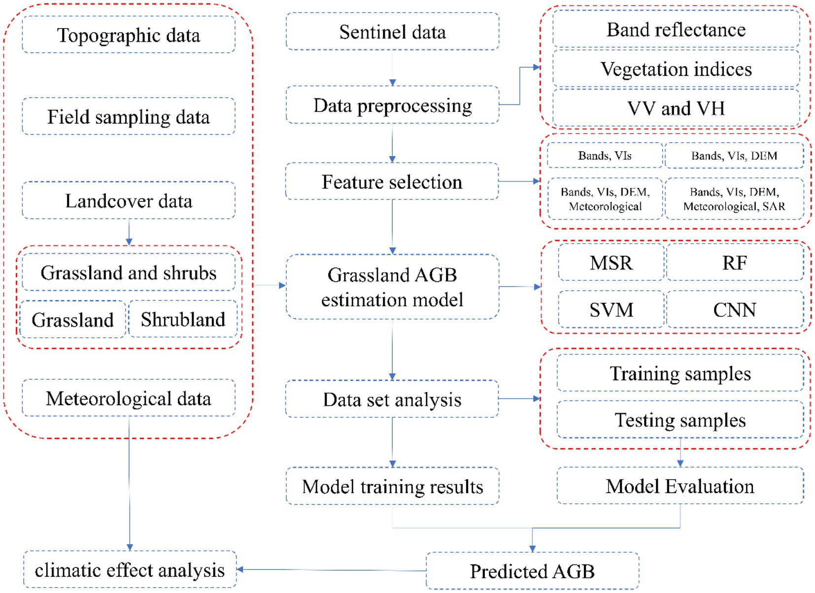
Figure 2. The technical flowchart of grassland AGB estimation in this study.
The field sample plots were divided into two subsets with approximately three-fourths of the plots used for model training (N is 214 and 158 in grassland and shrubland, respectively) and the others used for model validation (N = 84 in grassland and N = 63 in shrubland). In this study, the coefficient of determination (R2), root mean square error (RMSE) and mean absolute percentage error (MAPE) were calculated for evaluating the performance of prediction models. In addition, the 1:1 line was used to measure how far the ground-measured AGB values deviated from the predicted AGB values. A detailed description of the assessment indicators is shown as follows:
where n is the number of sample plots, and are the field measured and predicted AGB of plots i. is the mean measured AGB of all plots.
Partial correlation analysis is a process of eliminating the effect of the third variable when two variables are simultaneously correlated with the third variable and only analyzing the linear correlation between the two variables, which is commonly applied to assess the influences of climate change to the variation of grassland AGB (Guo et al., 2021; Xu et al., 2022). We applied it to determine the respective effects of temperature and precipitation on the differences of AGB distribution, with the indicator calculated as follows:
where is the partial correlation coefficient between variable x and variable y after excluding the influence of variable z. , and represent the Pearson correlation coefficients between each pair of AGB, temperature and precipitation, respectively, which is calculated as follows:
where and are the value of variable x and y in the year i; and represent the mean value of variable x and y from 2018 to 2022;
Additionally, a t-test is applied to test the significance of the partial correlation coefficient at a significance level of 0.05.
Overall, the biomass of shrubland was about 3 times higher than that of grassland, but the variation was large. According to ground sample plots, the measured AGB of shrubland had a wider range (from 648.9 to 3742.9 g/m2), with a mean AGB of 1829.2 g/m2, while the grassland AGB ranged from 202.4 to 1289.6 g/m2 with an average of 672.5 g/m2 (Table 2). Meanwhile, the AGB of shrubland also showed a larger standard deviation (751 g/m2) than that in grassland (265.8 g/m2), but their coefficient of variation (CV) was similar; 41 and 40% in shrubland and grassland, respectively. The high STD and CV were indicative of the high spatial heterogeneity in the study area.
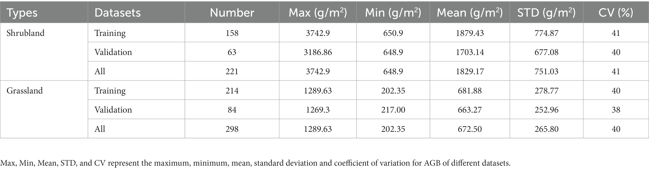
Table 2. The statistical descriptions of the measured AGB for the training set, validation set and all data of grassland and shrubland.
The four grassland AGB estimation models (MSR, RF, SVM and CNN) showed comparable results in the two modelling scenarios (Scenario 1: modelling all samples of grassland and shrubland together or Scenario 2: separately modelling them; Figure 3). We chose best model and better modelling scenarios through the following steps. (1) In general, the performance of CNN (testing R2 ranging from 0.7 to 0.82) and RF (testing R2 ranging from 0.64 to 0.8) models were significantly better than MSR (testing R2 ranging from 0.33 to 0.42) and SVM (testing R2 ranging from 0.45 to 0.64). (2) As compared to Scenario 1 (R2 was 0.7 and 0.64 for CNN and RF, respectively), both CNN (R2 was 0.72 and 0.82 for grassland and shrubland, respectively) and RF (R2 was 0.75 and 0.8 for grassland and shrubland, respectively) algorithms performed better in Scenario 2. (3) Since the R2 were very close for CNN and RF in Scenario 2, the comparisons of RMSE suggested that RF (131.2 and 267.8 g/m2 for grassland and shrubland, respectively) was superior over CNN (152.4 and 315.4 g/m2 for grassland and shrubland, respectively), reducing RMSE 14 and 15% for modeling AGB of grassland and shrubs, respectively. In summary, separately modelling grassland and shrubland by RF model was the best approach for AGB estimations in this study.
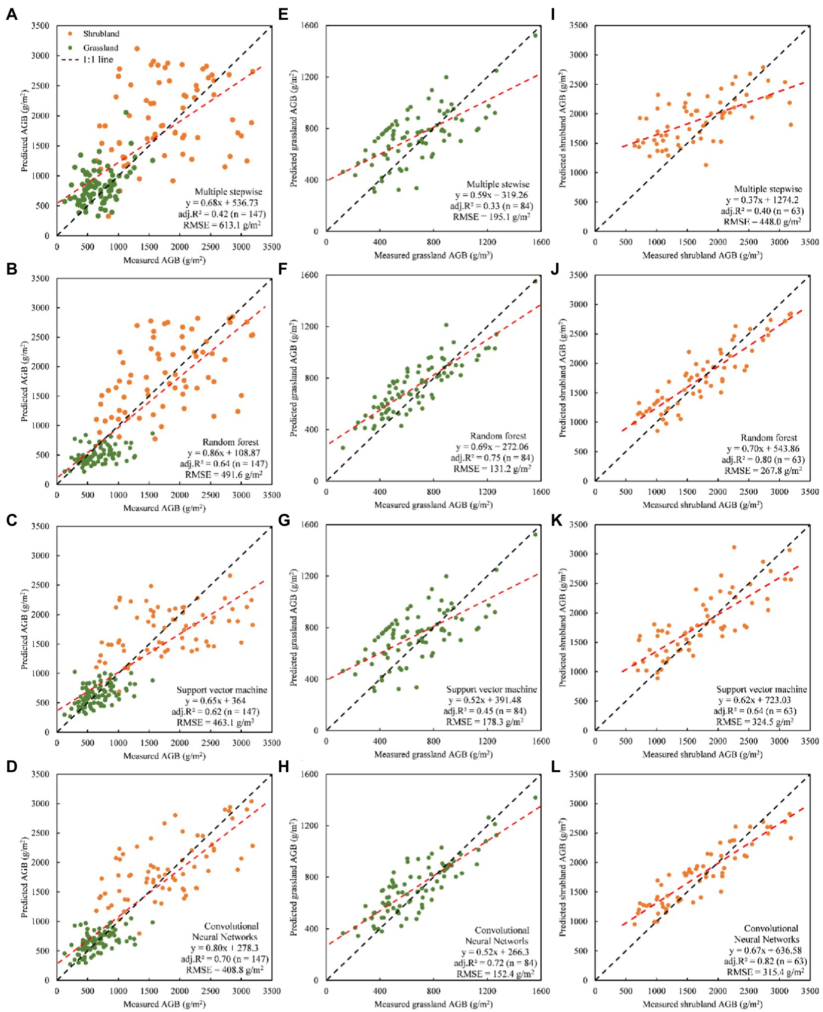
Figure 3. Scatter plot between measured and predicted AGB using the various prediction models in two modelling scenarios [Scenario 1: modelling all samples of grassland and shrubland together (A–D); Scenario 2: separately modelling grassland (E–H) and shrubland (I–L)].
Since the RF was the most suitable model in this study, the importance of input variables for RF was calculated (Figure 4). Some differences between grassland and shrubland for the top 10 most important factors were found. Compared with shrubland, the VIs were more important for monitoring grassland AGB using RF. There were 6 indices (EVI, EVI2, NDVI, NIRv, MSR, and DVI) in the top 10 factors, with EVI being the most important factor for predicting grassland AGB. Short-wavelength infrared bands (SWIR1 and SWIR2) were more important than the visible and near-infrared bands. Furthermore, Water VP and LST were also important in RF model for estimating grassland AGB. For shrubland, elevation was the most important biogeographical parameter affecting AGB (12.7% IncMSE), while VH was the least important variable (11.3% IncMSE), which was not reflected in the estimate of grassland AGB. The important VIs in shrubland were GCC, SR, DVI, EVI2, kNDVI, which was distinct from grassland. Additionally, Edge 3 was the most important spectral band for shrubland AGB estimation.
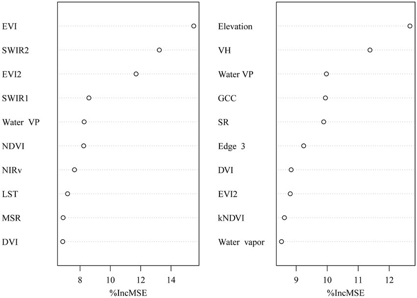
Figure 4. Importance (increase in mean squared error, %IncMSE) of input variables for random forest model in AGB estimation for grassland and shrubland.
High resolution optical images (Sentinel-2), SAR images (Sentinel-1), environmental and topographic data were major features to predict AGB of grassland by using the ML model. Since the RF model was superior among all eight ML models, the testing of the best combinations of input variables was carried out for regional AGB estimation. As shown in Table 3, all feature groups correlated strongly with validation AGB of grassland and shrubland, with R2 ranging from 0.60 to 0.75 and 0.54 to 0.8 for grassland and shrubland, respectively. Although it was obvious that the AGB model performed the best when all features were used as input variables, with the addition of SAR data into the AGB model of shrubland leading to the greatest improvement, increasing the accuracy expressed by the value of R2 from 0.57 to 0.68, while RMSE decreased from 454.1 to 332.7 g/m2.
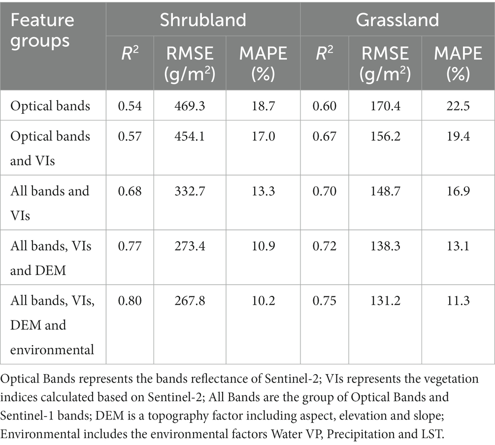
Table 3. Performance of various feature groups for AGB estimation using random forest.
Other than the remote sensing images of the Sentinel series, we also explored effects of spatial resolution variation on AGB estimation accuracy. MODIS data with 250 m resolution was used to instead of Sentinel without any other modifications to the RF model. This resulted in R2 values sustainably decreasing from 0.75 to 0.47 and 0.8 to 0.53 for grassland and shrubland, respectively (Figure 5; Table 3), demonstrating that the remote sensing source with better-detailed imaging was much more suitable for AGB estimation in this mountain grassland.
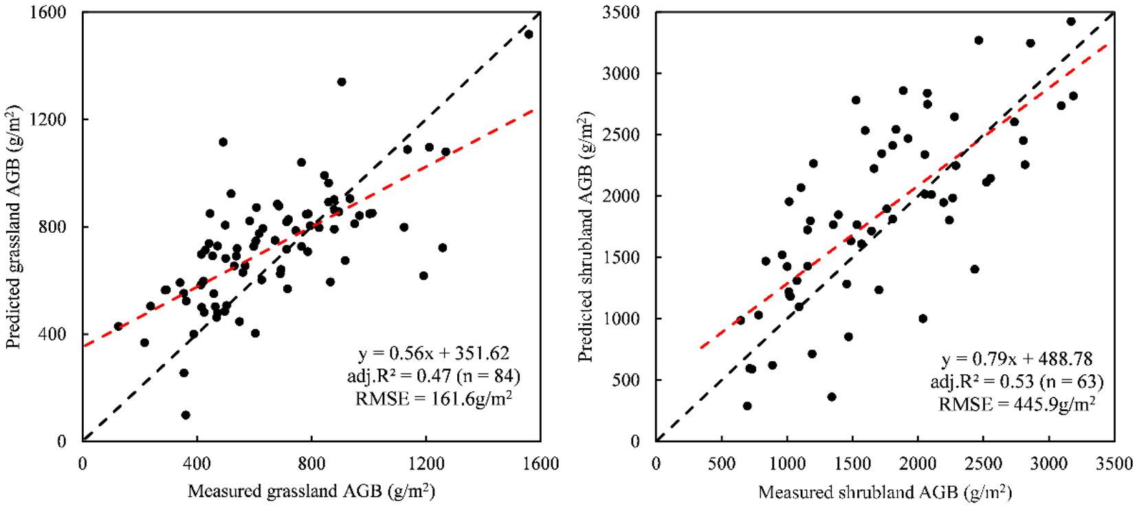
Figure 5. Scatter plot between measured and predicted AGB for grassland and shrubland using the RF based on the MODIS data with 250 m spatial resolution.
The AGB of grassland and shrubland across our study area in 2021 was predicted by best by the RF model (Figure 6). AGB of grassland and shrubland showed a similar spatial distribution with lower values distributed in the northwest and higher AGB in the central region, especially in the west of Guizhou province. The predicted mean grassland AGB was 596.1 g/m2 (STD was 209.5 g/m2) and most AGB values were concentrated in the ranges between 400 g/m2 and 900 g/m2 (as shown by the pixel frequency in the figure), which covered over half of the grassland area. The mean AGB was lower in Yunnan province (mean ± STD = 443.6 g/m2 ± 224.8 g/m2) than in Guizhou province (mean ± STD = 687.6 g/m2 ± 258.5 g/m2). The shrubland had higher mean AGB (1728.3 g/m2) and STD (470.8 g/m2) than grassland. The range of the predicted AGB for shrubland was 107.3–3473.6 g/m2 with over 70% of the shrubland area having AGB between 900 and 2,100 g/m2. The mean shrubland AGB in Guizhou province (mean ± STD = 1244.2 ± 466.8 g/m2) was also higher than that in Yunnan province (mean ± STD = 2303.9 ± 502.7 g/m2).
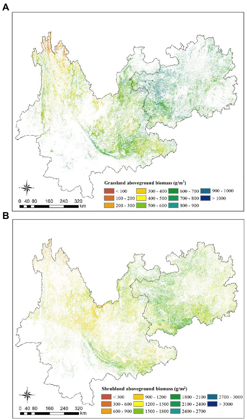
Figure 6. Spatial distribution of AGB of grassland (A) and shrubland (B) in Yunnan and Guizhou provinces in 2021.
We further analyzed the influences of topography (elevation and slope) on the spatial patter of AGB in the southwest mountainous area (Figure 7). The mean AGB of grassland and shrubland tended to decrease with increasing elevation. However, a lower mean AGB was found in the grassland elevation below 1,000 m, which might be affected by human activities like grazing and mowing. There were different influences of slope for the distribution of grassland and shrubland AGB. Slope barely affected the distribution of grassland AGB and the mean AGB was almost uniform (714.5 g/m2 in the slope range of 30–35 degrees and 850.7 g/m2 in the slope range of 20–25 degrees) across all ranges. By comparison, mean AGB of shrubland was highest in the flat area (2768.6 g/m2 in the slope less than 5 degree) and tended to decrease as the slope gets steeper (1755.9 g/m2 in the slope more than 35 degree).
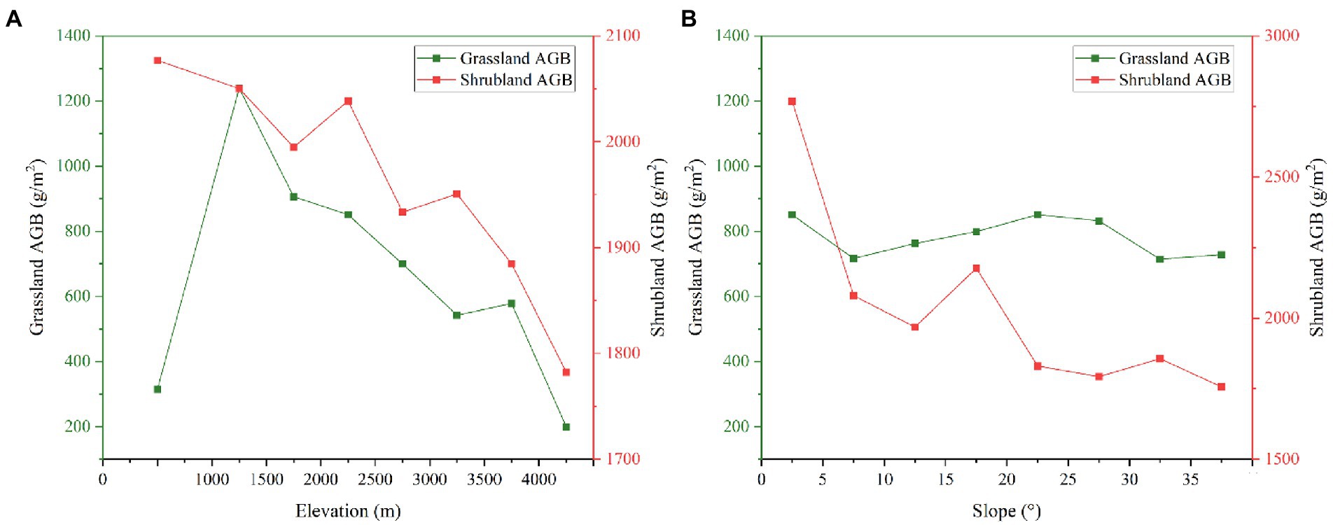
Figure 7. The variation of grassland and shrubland AGB along the elevation (A) and slope (B).
Precipitation and temperature are the most important climate factors affecting grassland growth. By using the RF model, we estimated AGB for five consecutive years (2018–2022) and then applied partial correlation analysis to calculate spatial correlations of AGB with mean annual temperature (MAT) and mean annual precipitation (MAP) in grassland and shrubland of this area. The results suggested a large spatial distribution variation regarding the influence of climatic factors on AGB (Figure 8). Generally, the positive relationship between AGB and MAP existed in a large proportion (70.3%) of the grassland, and 62.8% of which showed positive response to MAT (Table 4). In terms of spatial distribution, grasslands with significant positive correlation between two climate factors (MAP and MAT) and AGB were mainly concentrated in the central part of the study area (the boundary region of these two provinces), which accounted for over 29.4 and 29.5% area, respectively. Opposite effects of MAT and MAP on AGB were detected mainly in the southern and western regions. For shrubland, AGB showed a positive or significant positive correlation with MAP and MAT across 60.1 and 55.6% of the shrubland area, respectively, mainly in the central region.
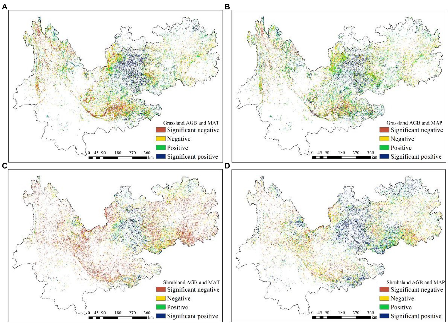
Figure 8. Partial correlation between grassland AGB and mean annual temperature (A), grassland AGB and mean annual precipitation (B), shrubland AGB and mean annual temperature (C), shrubland AGB and mean annual precipitation (D) at the significance level of 0.05 from 2018 to 2022.
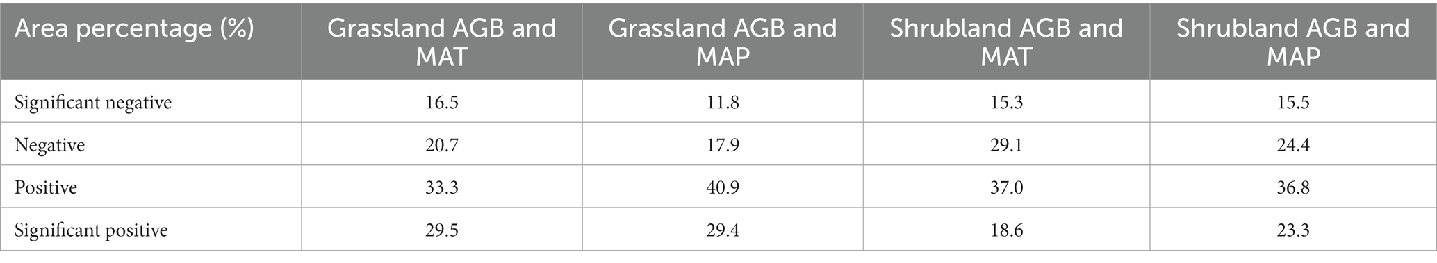
Table 4. Statistics of area percentage with different Influence of climate factors on AGB for grassland and shrubland: different relationships in different areas.
Moreover, we calculated the AGB responses to climatic factors along the temperature and precipitation gradient along 2°C (MAT) and 200 mm (MAP) steps. The results shown in Figure 9 indicated that there was a parabolical correlation between MAT and AGB of both grassland and shrubland (R2 = 0.86, p < 0.05 and R2 = 0.97, p < 0.05 for grassland and shrubland, respectively). More specifically, AGB of grassland and shrubland showed significant increasing trends below 19 and 18°C, respectively, (purple line in Figure 8A,C), and gradually decreased when temperature above 19 and 24°C, respectively (green line). Meanwhile, generally positive linear correlations between MAP and AGB of grassland and shrubland were observed (R2 = 0.55, p < 0.05 and R2 = 0.57, p < 0.05 for grassland and shrubland, respectively); however, turning points were observed in the relationships. Below MAP of 1,300 and 1,200 mm for grassland and shrubland, respectively, AGB significantly increased with MAP; when MAP was above these values, AGB exhibited slightly decreasing trends with precipitation (Figures 8B,D).
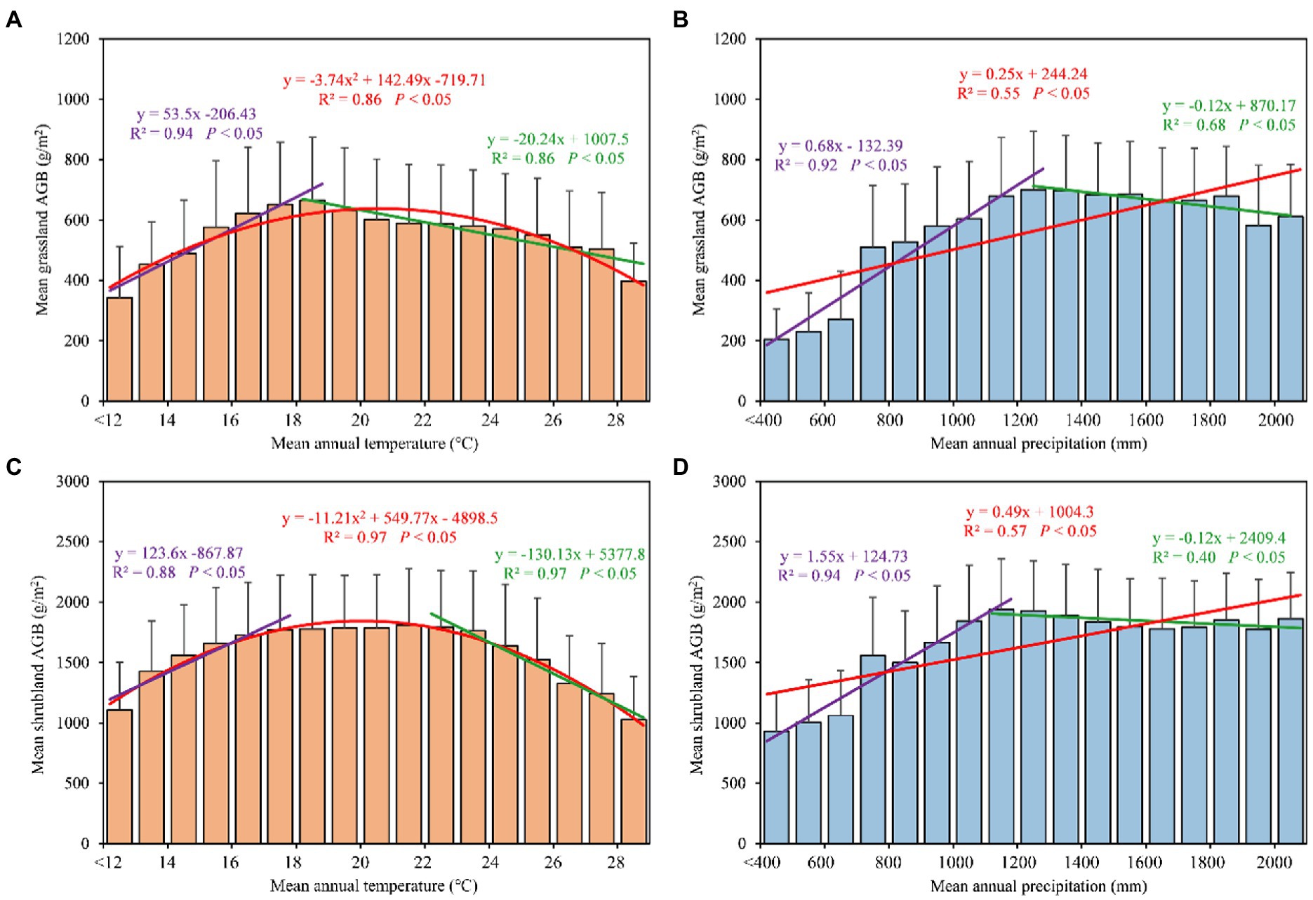
Figure 9. Relationship of average AGB of grassland (A and B) and shrubland (C and D) with MAT (2°C) and MAP (200 mm) gradients data from 2018 to 2022.
Numerous studies have demonstrated that ML models are a reliable tool in grassland AGB prediction due to their powerful interpretation ability and high efficiency (Zhang et al., 2015; Cheng et al., 2022). However, few studies have been conducted in mountain grassland due to its complex vegetation structure and topography (Cheng et al., 2022). In this study, four models were developed and tested for grassland AGB estimation on the Yunnan-Guizhou plateau. We found that due to the high landscape heterogeneity in this mountain grassland, separately modelling the pure grassland and shrubland yielded the best results. Among all AGB estimation algorithms, the ML and DL models had better accuracy than the traditional regression model. In this study, RF and CNN both produced encouraging results for grassland (R2 was 0.75 and 0.7 for RF and CNN, respectively) and shrubland (R2 was 0.8 and 0.82 for RF and CNN, respectively; Figure 3), with RF and its lower RMSE than CNN (14 and 15% lower in grassland and shrubland, respectively) achieving the best performance in grassland AGB estimation in Southwest China overall. These results were consistent with previous studies, suggesting that ML models, which have the advantage of accurately estimating complex non-linear relationship across variables, were more effective in dealing with multiple factors than ordinary regression models (Idowu et al., 2016; Lyu et al., 2021). Among ML models, some case studies have indicated that RF model performed better than other ML models in AGB estimation of grassland. Wang et al. (2017) simulated grassland AGB in a semiarid grassland and found that the RF model had a higher accuracy as compared to SVM model. Tang et al. (2021) also showed the RF model was superior to SVM, PLSR and back-propagation artificial neural network (BP-ANN) in AGB monitoring of the headwater of the Yellow River grasslands. Some recent comparison studies on AGB estimation performance of DL and ML models suggested CNN algorithm was found to perform better than classical ML models (i.e., RF, SVM), due to CNN was more sensitive to changes in features (Du et al., 2021; Zhang et al., 2022). While another case study showed RF would obtain slightly better accuracy than CNN if the data was elaborately designed (Dong et al., 2020). In our study, attribute to the designed modelling strategy and RF model’s strong robust to noise and outliers of heterogeneous ecosystems (Anaya et al., 2009; Xu et al., 2019), RF was found to be the most suitable model in AGB estimation of the mountain grassland in Southwest China.
Varies environmental factors affecting grassland growth including climate, soil and topography are common input variables to ML models in grassland related studies (Meng et al., 2020; Wang et al., 2022). However, most of these studies used only a single remote sensing data source. Since SAR has advantages in obtaining vegetation structure information, we introduced Sentinel-1 SAR images in our study area, where the grassland is highly mixed with shrubs. In this study, VIs played a more important role in pure grassland estimation, and the EVI and SWIR contributed the most among VIs in the RF model (Figure 4). Some previous research suggested that although EVI did not inevitably outperform NDVI in grassland mapping and AGB estimation, EVI was still an improvement with regards to obtaining more reasonable values in different vegetation density situation (Liu et al., 2014), and SWIR was the most relevant index for grassland extraction in mountain grassland (Cheng et al., 2022). In contrast, elevation and backscatter values from vertical and horizontal (VH) polarization were the two most important input variables for the shrubland AGB estimation model, which suggested shrubland biomass was greatly influenced by topography and vegetation structure in Southwest China. Some studies also reported that VH polarization data from Sentinel-1 SAR image had a higher accuracy than VV polarization data in biomass estimation (Liu et al., 2019). Moreover, the AGB estimation accuracy (R2) of shrubland significantly improved from 0.57 to 0.68 while reducing RMSE by 26.7% when Sentinel-1 SAR was introduced to the RF model. However, recent case studies have reported conflicting outcomes regarding the performance of combining SAR in grassland AGB estimation. For example, Wang et al. (2019) indicated that the integration of Sentinel-1, Landsat 8, and Sentinel-2 improved the estimation of AGB by more than 30% compared to using only Sentinel-1 in a native pasture of Oklahoma, USA; However, study by Chiarito et al. (2021) showed there was only a slight improvement when Sentinel-1 SAR was included in alpine meadows in Italy. Finally, While Raab et al. (2020) even reported no positive effect on the model performance by combining Sentinel-1 and Sentinel-2 data in semi-natural grasslands of Germany. Nevertheless, our research demonstrated the potential of combining SAR and high-resolution optical data to provide accurate AGB estimation in shrubs mixed mountain grassland.
Climate factors including precipitation and temperature are main drivers of biophysical processes and growth in grassland ecosystems. There is a strong positive linear relationship between AGB and MAP based on long-term observations in almost all grassland ecosystems (Bai et al., 2004; Knapp et al., 2017). However, increasing studies have suggested that the response of AGB to MAP would saturate under extreme wet conditions and the AGB-MAP linear relationship would be modified (Wilcox et al., 2016; Flombaum et al., 2017). For example, Hao et al. (2017) presented that AGB did not show a significant increase when growing season precipitation increased to extremely high values based on near 40 years long-term inventory data in a semiarid grassland. In this study, a general positive linear correlation between MAP and AGB was found for both grassland and shrubland. However, when MAP exceeded 1,300 and 1,200 mm for grassland and shrubland, respectively, AGB showed a slight decreasing trend rather than increasing further with MAP. Zeng et al. (2019) reported a similar relationship between MAP and AGB on the Tibetan Plateau. The spatial distribution of the MAP-AGB relationship indicated that the AGB of grassland (70%) and shrubs (60%) responded generally positively to MAP. Shrubland were less sensitive to climate factors than grassland, as evidenced by the lower proportion of areas where significant responses were found. According to a recent field study in central Yunnan province, MAP and MAT did not directly affect shrubland biomass and the ratio of root and shoot, but changed the relationship between the stoichiometric characteristics and environmental factors (Guo et al., 2022).
Clear parabolical correlations between AGB and MAT were observed for both grassland and shrubland. The turning point of grassland AGB along the temperature gradient was around 19°C, while shrubland AGB would gradually decrease when temperatures exceeded 24°C, which confirmed that shrubland were more tolerant to higher temperatures than grassland. Around 63% of grassland and 56% of shrubland showed a positive correlation with MAT, which for both was lower than the area positively correlated with MAP. This suggests that MAP played a more positive role for grass and shrub growth than MAT. Since extreme temperatures are occurring more frequently in this region under climate change (Yan et al., 2021), increasing drought risks to be amplified by heatwaves and thus threaten ecosystem functioning and human welfare.
Our study demonstrated that the integration of SAR and high-resolution optical remote sensing data into the random forest model can yield better performance in mountain grassland AGB estimation in Southwest China. The combination of multi-source remote sensing data provided an opportunity to monitor AGB from a multi-dimensional perspective. Additional satellite data, such as satellite-based hyperspectral and LiDAR data from multi-platforms, can further improve the correct inclusion of vegetation biochemical and structural features, which would lead to further increases in accuracy of grassland AGB estimation in the future. Furthermore, soil percentage in each pixel due to land fragmentation should also be noted, as this causes the uncertainty of the band reflectance and vegetation indices. The use of multi-temporal data could be considered as an approach by acquiring the soil information in the pre-growing season and eliminating or reducing its effects based on pixel unmixing (Li et al., 2016). Additionally, Sentinel series images were fully available in our study area after 2018, and the 5 years of data were able to use in this study is still too short for thorough climate related analyses, and may thus introduce some uncertainty. In fact, the spatial resolution of climate data is relatively coarse (1 km) and it is worth considering the fusion of high precision data (Sentinel) and long time series data such as MODIS data to produce long time series AGB spatial distribution dataset with high precision for a more accurate analysis of the influence of climate variables on AGB in the past time. This could enable refined management and sustainable development strategies for grassland.
AGB is one of the key indicators for grassland ecosystem research and management. In this study, we constructed and compared four remote sensing estimation model including a traditional regression model (multiple stepwise regression, MSR), two classical machine learning models (random forest, RF and supporting vector machine, SVM) and a deep learning model (convolutional neural network, CNN) to estimate grassland AGB in Yunnan and Guizhou Provinces, Southwest China. Our study suggests that separately modelling AGB of pure grassland and shrubland achieved better results than modelling them together. Among all test models, the RF model with input variables from field survey, high-resolution optical data (Sentinel-2), SAR data (Sentinel-1), environmental data and topographic data led to the best performance for AGB estimation of both grassland and shrubland. Among all input variables in the RF model, the vegetation indices (i.e., EVI, EVI2, and NDVI) were the most important for grassland AGB estimation, while topographical factor (i.e., elevation) and SAR data (i.e., VH band) contributed the most to the shrubland AGB estimation model. We also demonstrated that integrating the SAR data into input variables had great potential to improve the accuracy of AGB estimation, especially for shrubland, improving AGB estimation by 21%. Regional grassland AGB mapping showed high spatial heterogeneity, with lower values distributed in the Northwest and higher AGB in the central region. The mean AGB of grassland was lower in Yunnan Province (443.6 g/m2) than that in Guizhou Province (687.6 g/m2) in 2021. The climatic effects on AGB variation showed that there was a positive linear correlation with MAP, but a parabolical correlation with MAT for both grassland and shrubland AGB based on the estimation of grassland AGB in Southwest China from 2018 to 2022. This study provides an effective and accurate method to estimate mountain grassland AGB and offers a new insight to better understanding spatial variation in grassland AGB and its response to climatic factors in Southwest China.
The original contributions presented in the study are included in the article/supplementary material, further inquiries can be directed to the corresponding author.
All authors listed have made a substantial, direct, and intellectual contribution to the work and approved it for publication.
This research was funded by the China Geological Survey Project (ZD20220133), the National Natural Science Foundation of China (32260300), and the Project for Talent and Platform of Science and Technology in Yunnan Province Science and Technology Department (202205AM070005).
Authors would like to thank the support of provincial for Bama Snow Mountain vertical complex ecosystem research station during the field sample, contributions of Rongxiao Che for language editing, Hongwei Zeng’s advice for manuscript revising and the reviewers for their very helpful comments, suggestions that substantially improved the paper.
The authors declare that the research was conducted in the absence of any commercial or financial relationships that could be construed as a potential conflict of interest.
All claims expressed in this article are solely those of the authors and do not necessarily represent those of their affiliated organizations, or those of the publisher, the editors and the reviewers. Any product that may be evaluated in this article, or claim that may be made by its manufacturer, is not guaranteed or endorsed by the publisher.
Ali, I., Cawkwell, F., Dwyer, E., Barrett, B., and Green, S. (2016). Satellite remote sensing of grasslands: from observation to management. J. Plant Ecol. 9, 649–671. doi: 10.1093/jpe/rtw005
Anaya, J. A., Chuvieco, E., and Palacios-Orueta, A. (2009). Aboveground biomass assessment in Colombia: a remote sensing approach. For. Ecol. Manag. 257, 1237–1246. doi: 10.1016/j.foreco.2008.11.016
Bai, Y. F., Han, X. G., Wu, J. G., Chen, Z. Z., and Li, L. H. (2004). Ecosystem stability and compensatory effects in the Inner Mongolia grassland. Nature 431, 181–184. doi: 10.1038/nature02850
Barrett, B., Nitze, I., Green, S., and Cawkwell, F. (2014). Assessment of multi-temporal, multi-sensor radar and ancillary spatial data for grasslands monitoring in Ireland using machine learning approaches. Remote Sens. Environ. 152, 109–124. doi: 10.1016/j.rse.2014.05.018
Cheng, X., Liu, W., Zhou, J., Wang, Z., Zhang, S., and Liao, S. (2022). Extraction of mountain grasslands in Yunnan, China, from sentinel-2 data during the optimal phenological period using feature optimization. Agronomy 12:1948. doi: 10.3390/agronomy12081948
Chiarito, E., Cigna, F., Cuozzo, G., Fontanelli, G., Mejia Aguilar, A., Paloscia, S., et al. (2021). Biomass retrieval based on genetic algorithm feature selection and support vector regression in Alpine grassland using ground-based hyperspectral and Sentinel-1 Sar data. Eur. J. Remote Sens. 54, 209–225. doi: 10.1080/22797254.2021.1901063
Chu, Y., Wee, A. K. S., Lapuz, R. S., and Tomlinson, K. W. (2021). Phylogeography of two widespread C4 grass species suggest that tableland and valley grassy biome in southwestern China pre-date human modification. Glob. Ecol. Conserv. 31:e01835. doi: 10.1016/j.gecco.2021.e01835
Dong, L., Du, H., Han, N., Li, X., Zhu, D. E., Mao, F., et al. (2020). Application of convolutional neural network on lei bamboo above-ground-biomass (Agb) estimation using Worldview-2. Remote Sens. 12:958. doi: 10.3390/rs12060958
Du, C., Fan, W., Ma, Y., Jin, H. I., and Zhen, Z. (2021). The effect of synergistic approaches of features and ensemble learning Algorith on aboveground biomass estimation of natural secondary forests based on Als and Landsat 8. Sensors 21, 5974–6002. doi: 10.3390/s21175974
Elnashar, A., Zeng, H., Wu, B., Zhang, N., Tian, F., Zhang, M., et al. (2020). Downscaling Trmm monthly precipitation using Google earth engine and Google cloud computing. Remote Sens. 12:3860. doi: 10.3390/rs12233860
Flombaum, P., and Sala, O. E. (2007). A non-destructive and rapid method to estimate biomass and aboveground net primary production in arid environments. J. Arid Environ. 69, 352–358. doi: 10.1016/j.jaridenv.2006.09.008
Flombaum, P., Yahdjian, L., and Sala, O. E. (2017). Global-change drivers of ecosystem functioning modulated by natural variability and saturating responses. Glob. Chang. Biol. 23, 503–511. doi: 10.1111/gcb.13441
Ge, J., Meng, B., Liang, T., Feng, Q., Gao, J., Yang, S., et al. (2018). Modeling alpine grassland cover based on Modis data and support vector machine regression in the headwater region of the Huanghe River, China. Remote Sens. Environ. 218, 162–173. doi: 10.1016/j.rse.2018.09.019
Guerschman, J. P., Hill, M. J., Renzullo, L. J., Barrett, D. J., Marks, A. S., and Botha, E. J. (2009). Estimating fractional cover of photosynthetic vegetation, non-photosynthetic vegetation and bare soil in the Australian tropical savanna region upscaling the Eo-1 Hyperion and Modis sensors. Remote Sens. Environ. 113, 928–945. doi: 10.1016/j.rse.2009.01.006
Guo, Z., Chen, W., Chen, Q., Liu, X., Hong, S., Zhu, X., et al. (2022). Biomass distribution pattern and stoichiometric characteristics in main shrub ecosystems in Central Yunnan, China. PeerJ 10:e13005. doi: 10.7717/peerj.13005
Guo, D., Song, X., Hu, R., Cai, S., Zhu, X., and Hao, Y. (2021). Grassland type-dependent spatiotemporal characteristics of productivity in Inner Mongolia and its response to climate factors. Sci. Total Environ. 775:145644. doi: 10.1016/j.scitotenv.2021.145644
Hao, Y. B., Zhou, C. T., Liu, W. J., Li, L. F., Kang, X. M., Jiang, L. L., et al. (2017). Aboveground net primary productivity and carbon balance remain stable under extreme precipitation events in a semiarid steppe ecosystem. Agric. For. Meteorol. 240-241, 1–9. doi: 10.1016/j.agrformet.2017.03.006
Idowu, S., Saguna, S., Åhlund, C., and Schelén, O. (2016). Applied machine learning: forecasting heat load in district heating system. Energ. Buildings 133, 478–488. doi: 10.1016/j.enbuild.2016.09.068
Jin, Y., Yang, X., Qiu, J., Li, J., Gao, T., Wu, Q., et al. (2014). Remote sensing-based biomass estimation and its spatio-temporal variations in temperate grassland, Northern China. Remote Sens. 6, 1496–1513. doi: 10.3390/rs6021496
Jordan, M. I., and Mitchell, T. M. (2015). Machine learning: trends, perspectives, and prospects. Science 349, 255–260. doi: 10.1126/science.aaa8415
Knapp, A. K., Ciais, P., and Smith, M. D. (2017). Reconciling inconsistencies in precipitation-productivity relationships: implications for climate change. New Phytol. 214, 41–47. doi: 10.1111/nph.14381
Krizhevsky, A., Sutskever, I., and Hinton, G. E. (2017). ImageNet classification with deep convolutional neural networks. Commun. ACM 60, 84–90. doi: 10.1145/3065386
Lecun, Y., Bengio, Y., and Hinton, G. (2015). Deep learning. Nature 521, 436–444. doi: 10.1038/nature14539
Li, F., Jiang, L., Wang, X., Zhang, X., Zheng, J., and Zhao, Q. (2013). Estimating grassland aboveground biomass using multitemporal Modis data in the West Songnen Plain, China. J. Appl. Remote. Sens. 7:073546. doi: 10.1117/1.Jrs.7.073546
Li, F., Zeng, Y., Luo, J., Ma, R., and Wu, B. (2016). Modeling grassland aboveground biomass using a pure vegetation index. Ecol. Indic. 62, 279–288. doi: 10.1016/j.ecolind.2015.11.005
Liu, Y., Gong, W., Xing, Y., Hu, X., and Gong, J. (2019). Estimation of the forest stand mean height and aboveground biomass in Northeast China using Sar sentinel-1B, multispectral sentinel-2A, and Dem imagery. ISPRS J. Photogramm. Remote Sens. 151, 277–289. doi: 10.1016/j.isprsjprs.2019.03.016
Liu, X., Zhang, J., Zhu, X., Pan, Y., Liu, Y., Zhang, D., et al. (2014). Spatiotemporal changes in vegetation coverage and its driving factors in the Three-River headwaters region during 2000–2011. J. Geogr. Sci. 24, 288–302. doi: 10.1007/s11442-014-1088-0
Lu, D. (2007). The potential and challenge of remote sensing-based biomass estimation. Int. J. Remote Sens. 27, 1297–1328. doi: 10.1080/01431160500486732
Lyu, X., Li, X., Gong, J., Li, S., Dou, H., Dang, D., et al. (2021). Remote-sensing inversion method for aboveground biomass of typical steppe in Inner Mongolia, China. Ecol. Indic. 120:106883. doi: 10.1016/j.ecolind.2020.106883
Meng, B., Liang, T., Yi, S., Yin, J., Cui, X., Ge, J., et al. (2020). Modeling alpine grassland above ground biomass based on remote sensing data and machine learning algorithm: a case study in east of the Tibetan Plateau, China. IEEE J. Sel. Top. Appl. Earth Observ. Remote Sens. 13, 2986–2995. doi: 10.1109/JSTARS.2020.2999348
Morais, T. G., Teixeira, R. F. M., Figueiredo, M., and Domingos, T. (2021). The use of machine learning methods to estimate aboveground biomass of grasslands: a review. Ecol. Indic. 130:108081. doi: 10.1016/j.ecolind.2021.108081
Mu, J., Zeng, Y., Wu, Q., Niklas, K. J., and Niu, K. (2016). Traditional grazing regimes promote biodiversity and increase nectar production in Tibetan alpine meadows. Agric. Ecosyst. Environ. 233, 336–342. doi: 10.1016/j.agee.2016.09.030
Naidoo, L., Van Deventer, H., Ramoelo, A., Mathieu, R., Nondlazi, B., and Gangat, R. (2019). Estimating above ground biomass as an indicator of carbon storage in vegetated wetlands of the grassland biome of South Africa. Int. J. Appl. Earth Obs. Geoinf. 78, 118–129. doi: 10.1016/j.jag.2019.01.021
Niu, K., Choler, P., De Bello, F., Mirotchnick, N., Du, G., and Sun, S. (2014). Fertilization decreases species diversity but increases functional diversity: a three-year experiment in a Tibetan alpine meadow. Agric. Ecosyst. Environ. 182, 106–112. doi: 10.1016/j.agee.2013.07.015
Powell, S. L., Cohen, W. B., Healey, S. P., Kennedy, R. E., Moisen, G. G., Pierce, K. B., et al. (2010). Quantification of live aboveground forest biomass dynamics with Landsat time-series and field inventory data: a comparison of empirical modeling approaches. Remote Sens. Environ. 114, 1053–1068. doi: 10.1016/j.rse.2009.12.018
Quan, X., He, B., Yebra, M., Yin, C., Liao, Z., Zhang, X., et al. (2017). A radiative transfer model-based method for the estimation of grassland aboveground biomass. Int. J. Appl. Earth Obs. Geoinf. 54, 159–168. doi: 10.1016/j.jag.2016.10.002
Raab, C., Riesch, F., Tonn, B., Barrett, B., Meißner, M., Balkenhol, N., et al. (2020). Target-oriented habitat and wildlife management: estimating forage quantity and quality of semi-natural grasslands with Sentinel-1 and Sentinel-2 data. Remote Sens. Ecol. Conserv. 6, 381–398. doi: 10.1002/rse2.149
Ramoelo, A., Cho, M. A., Mathieu, R., Madonsela, S., Van De Kerchove, R., Kaszta, Z., et al. (2015). Monitoring grass nutrients and biomass as indicators of rangeland quality and quantity using random forest modelling and WorldView-2 data. Int. J. Appl. Earth Obs. Geoinf. 43, 43–54. doi: 10.1016/j.jag.2014.12.010
Ren, H., Zhou, G., and Zhang, F. (2018). Using negative soil adjustment factor in soil-adjusted vegetation index (Savi) for aboveground living biomass estimation in arid grasslands. Remote Sens. Environ. 209, 439–445. doi: 10.1016/j.rse.2018.02.068
Scurlock, J. M. O., and Hall, D. O. (2002). The global carbon sink: a grassland perspective. Glob. Chang. Biol. 4, 229–233. doi: 10.1046/j.1365-2486.1998.00151.x
Shen, H. H., Zhu, Y. K., Zhao, X., Geng, X. Q., and Gao, S. Q. (2016). Analysis of current grassland resources in China. Chin. Sci. Bull. 61, 139–154. doi: 10.1360/N972015-00732
Sinha, S., Jeganathan, C., Sharma, L. K., and Nathawat, M. S. (2015). A review of radar remote sensing for biomass estimation. Int. J. Environ. Sci. Technol. 12, 1779–1792. doi: 10.1007/s13762-015-0750-0
Tang, R., Zhao, Y., and Lin, H. (2021). Spatio-temporal variation characteristics of aboveground biomass in the headwater of the Yellow River based on machine learning. Remote Sens. 13:3404. doi: 10.3390/rs13173404
Wang, P., Fan, E., and Wang, P. (2021). Comparative analysis of image classification algorithms based on traditional machine learning and deep learning. Pattern Recogn. Lett. 141, 61–67. doi: 10.1016/j.patrec.2020.07.042
Wang, Y., Qin, R., Cheng, H., Liang, T., Zhang, K., Chai, N., et al. (2022). Can machine learning algorithms successfully predict grassland aboveground biomass? Remote Sens. 14:3843. doi: 10.3390/rs14163843
Wang, Y., Wang, G., Wu, Q., Niu, F., and Cheng, H. (2010). The impact of vegetation degeneration on hydrology features of alpine soil. J. Glaciol. Geocryol. 32, 989–998. doi: 10.1080/00949651003724790
Wang, Y., Wu, G., Deng, L., Tang, Z., Wang, K., Sun, W., et al. (2017). Prediction of aboveground grassland biomass on the loess plateau, China, using a random forest algorithm. Sci. Rep. 7:6940. doi: 10.1038/s41598-017-07197-6
Wang, J., Xiao, X., Bajgain, R., Starks, P., Steiner, J., Doughty, R. B., et al. (2019). Estimating leaf area index and aboveground biomass of grazing pastures using Sentinel-1, Sentinel-2 and Landsat images. ISPRS J. Photogramm. Remote Sens. 154, 189–201. doi: 10.1016/j.isprsjprs.2019.06.007
Wei, P., Chen, S., Wu, M., Jia, Y., Xu, H., and Liu, D. (2021). Increased ecosystem carbon storage between 2001 and 2019 in the northeastern margin of the Qinghai-Tibet plateau. Remote Sens. 13:3986. doi: 10.3390/rs13193986
Wilcox, K. R., Blair, J. M., Smith, M. D., and Knapp, A. K. (2016). Does ecosystem sensitivity to precipitation at the site-level conform to regional-scale predictions? Ecology 97, 561–568. doi: 10.1890/15-1437.1
Wu, B. F., Qian, J., and Zeng, Y. (2017). Land cover atlas of the People’s republic of China (1:1,000,000). Beijing, Sinomaps Press.
Wu, C., Shen, H., Shen, A., Deng, J., Gan, M., Zhu, J., et al. (2016). Comparison of machine-learning methods for above-ground biomass estimation based on Landsat imagery. J. Appl. Remote. Sens. 10:035010. doi: 10.1117/1.JRS.10.035010
Xu, D., Chen, B., Shen, B., Wang, X., Yan, Y., Xu, L., et al. (2019). The classification of grassland types based on object-based image analysis with multisource data. Rangel. Ecol. Manag. 72, 318–326. doi: 10.1016/j.rama.2018.11.007
Xu, C., Liu, W., Zhao, D., Hao, Y., Xia, A., Yan, N., et al. (2022). Remote sensing-based spatiotemporal distribution of grassland aboveground biomass and its response to climate change in the Hindu Kush Himalayan Region. Chin. Geogr. Sci. 32, 759–775. doi: 10.1007/s11769-022-1299-8
Yan, W., He, Y., Cai, Y., Qu, X., and Cui, X. (2021). Relationship between extreme climate indices and spatiotemporal changes of vegetation on Yunnan Plateau from 1982 to 2019. Glob. Ecol. Conserv. 31:e01813. doi: 10.1016/j.gecco.2021.e01813
Yang, S., Feng, Q., Liang, T., Liu, B., Zhang, W., and Xie, H. (2018). Modeling grassland above-ground biomass based on artificial neural network and remote sensing in the Three-River headwaters region. Remote Sens. Environ. 204, 448–455. doi: 10.1016/j.rse.2017.10.011
Zeng, N., Ren, X., He, H., Zhang, L., Li, P., and Niu, Z. (2021). Estimating the grassland aboveground biomass in the Three-River Headwater Region of China using machine learning and Bayesian model averaging. Environ. Res. Lett. 16:16. doi: 10.1088/1748-9326/ac2e85
Zeng, N., Ren, X., He, H., Zhang, L., Zhao, D., Ge, R., et al. (2019). Estimating grassland aboveground biomass on the Tibetan plateau using a random forest algorithm. Ecol. Indic. 102, 479–487. doi: 10.1016/j.ecolind.2019.02.023
Zhang, C., Denka, S., Cooper, H., and Mishra, D. R. (2018). Quantification of sawgrass marsh aboveground biomass in the coastal Everglades using object-based ensemble analysis and Landsat data. Remote Sens. Environ. 204, 366–379. doi: 10.1016/j.rse.2017.10.018
Zhang, F., Tian, X., Zhang, H., and Jiang, M. (2022). Estimation of aboveground carbon density of forests using deep learning and multisource remote sensing. Remote Sens. 14:3022. doi: 10.3390/rs14133022
Keywords: aboveground biomass, grassland, shrubland, machine learning, SAR, climate
Citation: Liu W, Xu C, Zhang Z, De Boeck H, Wang Y, Zhang L, Xu X, Zhang C, Chen G and Xu C (2023) Machine learning-based grassland aboveground biomass estimation and its response to climate variation in Southwest China. Front. Ecol. Evol. 11:1146850. doi: 10.3389/fevo.2023.1146850
Edited by:
Zhongqing Yan, Chinese Academy of Forestry, ChinaReviewed by:
Guangbin Lei, Institute of Mountain Hazards and Environment (CAS), ChinaCopyright © 2023 Liu, Xu, Zhang, De Boeck, Wang, Zhang, Xu, Zhang, Chen and Xu. This is an open-access article distributed under the terms of the Creative Commons Attribution License (CC BY). The use, distribution or reproduction in other forums is permitted, provided the original author(s) and the copyright owner(s) are credited and that the original publication in this journal is cited, in accordance with accepted academic practice. No use, distribution or reproduction is permitted which does not comply with these terms.
*Correspondence: Can Xu, eHVjYW5AbWFpbC5jZ3MuZ292LmNu
Disclaimer: All claims expressed in this article are solely those of the authors and do not necessarily represent those of their affiliated organizations, or those of the publisher, the editors and the reviewers. Any product that may be evaluated in this article or claim that may be made by its manufacturer is not guaranteed or endorsed by the publisher.
Research integrity at Frontiers
Learn more about the work of our research integrity team to safeguard the quality of each article we publish.