Climate change alters the spatial pattern of plant spectral diversity across forest types

Species distribution, spatial distance, and neighboring interact6ions are among the most important drivers of global variation in plant species diversity. However, the effects of climate change on the relationship between spatial interactions and species diversity remain unknown. Here, we applied 12 machine learning models to assess the responses of spectral diversity (indicating species diversity) in forests in seven protected forest areas in China. Changes in 27 climatic variables during two time periods, 1990–2005 and 2005–2020, were analyzed. The results indicated that spectral diversity and intraspecific spatial distance have increased significantly with climate change. These results also provide insights into the variations in spectral diversity. Particularly, the contributions of neighboring interactions and plant–plant distances to the variation in species diversity between 1990 and 2000 were greater than the contribution of climate change in all forest types. Our analysis revealed that species diversity, plant–plant interactions, and spatial distance are closely associated with each other and sharply shifted under climate change. From this perspective, spatial interaction analysis—to a greater degree than analysis of community composition—can provide additional insights into the underlying mechanisms of changes in species diversity under current global-warming conditions.

1 Introduction

Global climate has been in a state of continuous warming for nearly a century. The current rate of temperature increase is approximately twice that of the previous century (Karl et al., 2015), and this increase is most pronounced at high elevations and latitudes (Peñuelas et al., 2013). Several studies have focused on the effects of climate change on plant diversity in different regions of the world (Boutin et al., 2017; Harrison et al., 2020). The species richness of vascular plants has also increased with the rise in temperature and nitrogen deposition, resulting in notable species-composition shifts (Boutin et al., 2017). In the Columbia River Gorge National Scenic Area, species richness, annual average temperature, and relative humidity were found to be significantly and positively related to each other (Matos et al., 2017). The higher the plant species diversity, the lower the impact of climate change (Li et al., 2018). Globally, regions with warm and wet climates support more species than those with cold or arid climates. This broad-scale climatic influence outweighs any other contributor to plant species diversity (Kreft & Jetz, 2007; Harrison et al., 2020). Reportedly, taxonomic diversity increases with increasing rainfall or varies with increasing productivity despite a slight decrease in temperature (Kreft & Jetz, 2007; Harrison et al., 2020). The relationship between woody species composition and climate is highly consistent across spatial scales and organizational levels (Kreft & Jetz, 2007; Harrison et al., 2020). Based on a very large dataset of six million trees in more than 180,000 field plots in central Africa, researchers have shown that sensitivity to climate change is the highest in endemic species-dominated forests and the driest forests (Réjou-Méchain et al., 2021). Further, recent studies in West Africa have shown that dry tropical forests exhibit larger functional changes compared with moist forests in response to long-term drought (Aguirre-Gutiérrez et al., 2019) and are likely to be more sensitive to global warming (Sullivan et al., 2020). In another study conducted in the Amazon, researchers found a peak in phylogenetic diversity at an intermediate level of precipitation (Neves et al., 2020). Conversely, forests dominated by widespread tree taxa adapted to anthropogenic pressures show relatively low sensitivity to climate change (Réjou-Méchain et al., 2021). Based on model predictions (Réjou-Méchain et al., 2021), undisturbed semi-deciduous and transitional forests appear phylogenetically more diverse than evergreen forests and demonstrate less sensitivity to climate change. However, these in-depth studies have mainly focused on the effects of climate change on plant species diversity in certain regions. Notably, an overall understanding of the spatial patterns of species diversity across vegetation types on a large scale remains lacking.

The measurement of species diversity on a large spatial scale is expected to be more time- and labor-intensive and expensive than on a small scale. With the use of remote sensing, it is now possible to monitor species diversity in large areas over a short period of time (Rocchini, 2007; Madonsela et al., 2017). Of the many different spectral vegetation indices that serve as proxy measures of species diversity, the coefficient of variation in the Normalized Difference Vegetation Index (CV-NDVI), which indicates the variation in spectral species within a plot, i.e., alpha diversity, is most widely used (Peng et al., 2019).

Forests are more appropriate for observing the effects of climate change than other ecosystems because trees have long growth stages and are less affected by occasional, short-term, or intravariable climatic fluctuations (Engler et al., 2009; Zwiener et al., 2018). Spectral diversity indices extracted from remote sensing imagery are particularly useful for predicting forest species diversity because the size of a tree crown usually matches well with the pixel size of satellite images. Furthermore, the use of protected areas (PAs) in this type of analysis can minimize non-climate anthropogenic impacts on plant diversity. An examination of the spatial distribution of plant species can help us to understand the mechanism of climate change impacting plant diversity and provide a reference for biodiversity conservation in world forests. In this study, we used spectral diversity (CV-NDVI) to evaluate plant species diversity. Based on the results of previous studies, we hypothesized the following: 1) species diversity could increase due to a rise in global temperature, associated with increased productivity; 2) increased plant diversity would produce strong neighboring effects, and plant–plant competition could become severe; 3) stronger neighboring interactions and plant–plant competition could lead to a longer spatial distance between plants, and the clustering community would become diffused; and 4) the changes in spatial distance and neighboring interactions could produce a feedback effect on species diversity (Figure 1). Using remote sensing techniques and spatial analysis, we tested our hypotheses based on the spectral diversity of vegetation in seven protected forests in China.

FIGURE 1

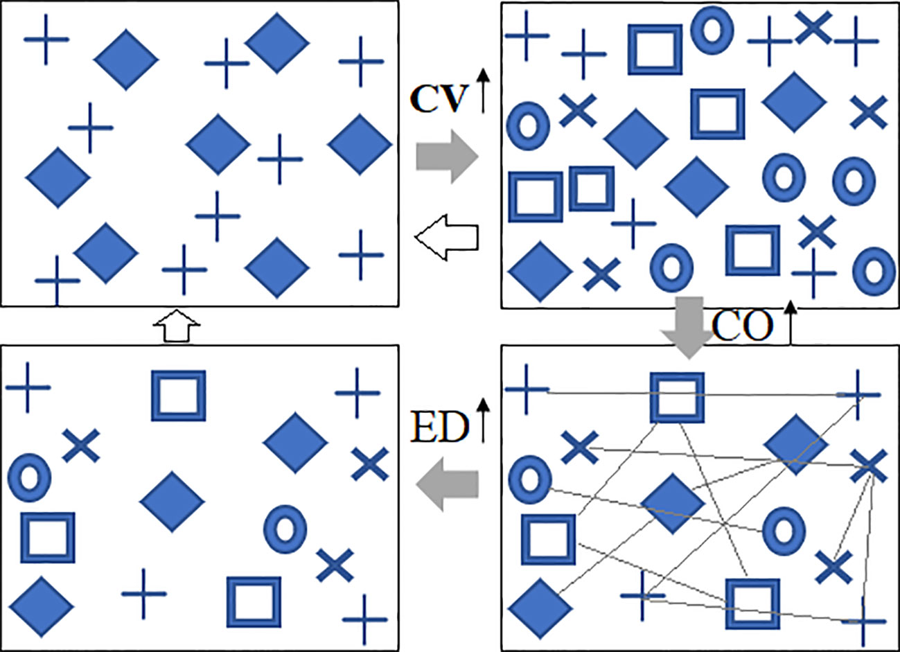
Figure 1 Conceptual illustrations of predicted changes in vegetation spectral diversity under climate warming. Under climate warming, species diversity (CV) could increase, the abundance of plants could increase, the neighboring interactions (CO) would become stronger, and, consequently, self-thinning effects will lead to a longer distance (ED) between two plants of the same species. The variation in ED and CO can also work on CV. Different symbols represent different spectral species; CV, spectral alpha diversity; CO, neighboring correlation; ED, spatial distance.

2 Study area and methods

2.1 Study area

For the present study, protected forest areas in China were selected as the data source based on the following criteria: 1) PAs established before 1980 to guarantee an undisturbed status of plant diversity in the area; 2) PAs having Landsat images in the growing seasons in 1990, 2005, and 2020, with a cloud cover of less than 10%; 3) PAs larger than 100 km², in which a core area with a buffer zone (larger than 2 km) can be created; and 4) PAs located entirely within one forest biome and not mixed with other forest types. These criteria were selected to ensure the quality of Landsat images, sufficient space for plot sampling, and the reliability of comparisons across different forest types. Out of all 474 national PAs, seven (with a median area of 100 km²) (Figure 2), representing a geographically stratified and broad selection of evergreen broad-leaved, deciduous, and needle-leaved forests from low to high latitudes (Ricklefs & He, 2016), were selected for this study.

FIGURE 2

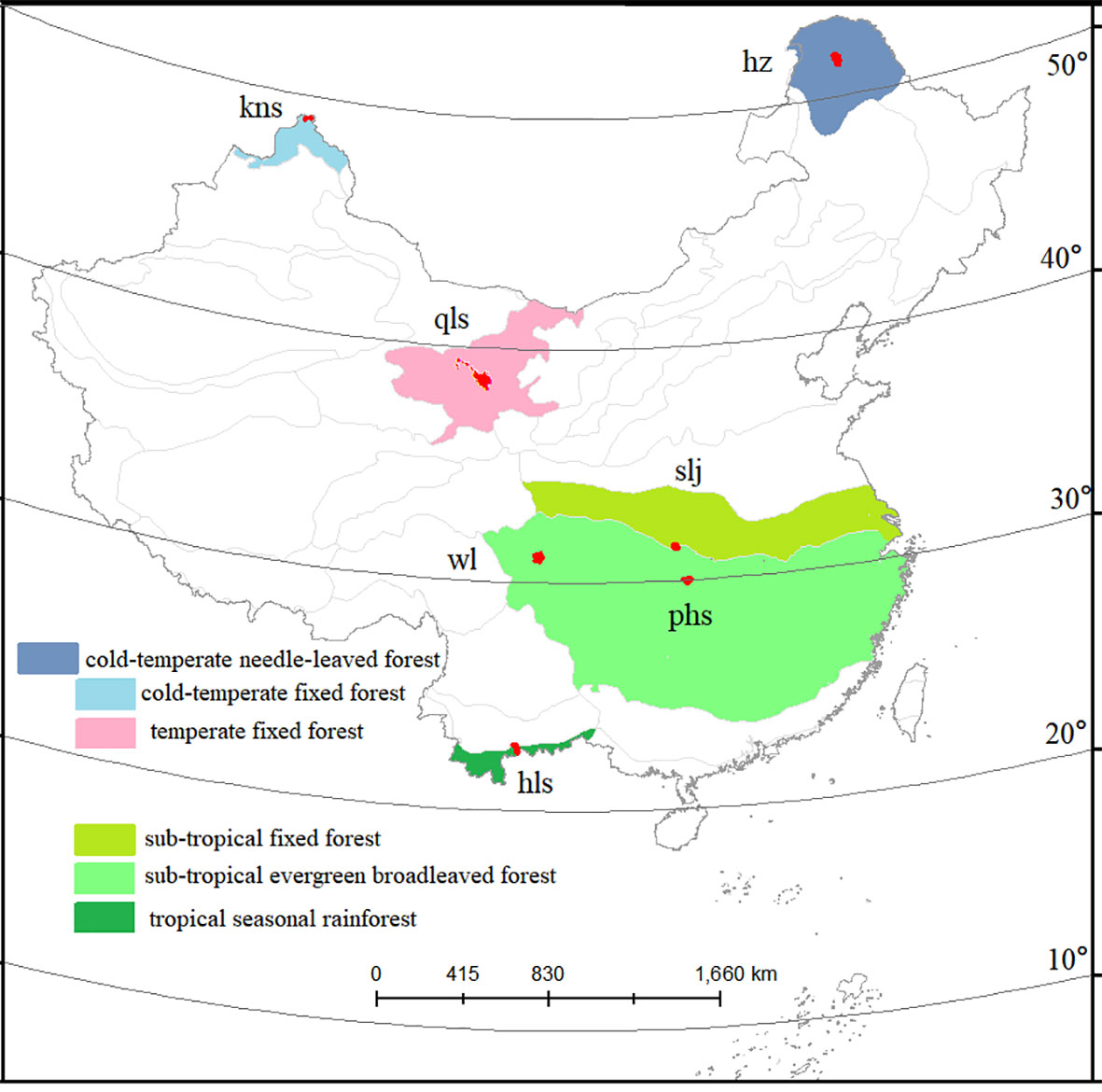
Figure 2 Study area. Seven protected forest areas across a latitudinal gradient. Forest types are indicated by colored areas.

2.2 Plant diversity indices derived from Landsat images

Prior to calculating the spectral diversity indices, all the Landsat images were processed. Cloud-free Landsat satellite images (with a spatial resolution of 30 m) were obtained for the years 1990, 2005, and 2020 from the Global Land Cover Facility website (http://glcfapp.umiacs.umd.edu). All Landsat images were radiometrically and atmospherically corrected using Idrisi GIS (Levin et al., 2007). Thereafter, the images were validated for shading effects at 30-m resolution caused by topography using the ASTER global digital elevation model (http://gdem.ersdac.jspacesystems.or.jp). In order to differentiate the biological features of forests while minimizing the problems of image incompatibility due to seasonal or annual differences, images during the growing seasons were included. Radiance values were converted to surface reflectance, which helped identify the differences in exoatmospheric irradiance and solar zenith angles (Rocchini, 2007; Duro et al., 2014). All image processing was performed using ERDAS Imagine software.

After pre-processing, the CV of the NDVI (CVn) within a window of 3 × 3 pixels was calculated as the spectral alpha diversity index of the plot. A series of spectral biodiversity indices (CVn) was then generated at plot sizes of 3 × 3, 5 × 5, 9 × 9, 17 × 17, and 33 × 33 pixels. After investigating the effects of spatial autocorrelation, estimation accuracy, and environmental scale, we selected a window of 33 × 33 pixels as the most convenient size to calculate spectral diversity, which has also been used in similar studies on tropical mountain rainforests (Wallis et al., 2017) and savannah woodlands (Madonsela et al., 2017).

2.3 Spectral–spatial metrics

From the NDVI imagery, we derived three spectral–spatial measures, namely, spatial distance, spatial aggregation, and neighboring correlation, as species spatial pattern representatives. The Euclidean nearest-neighbor distance (ED) represents the distance (m) from spectral plant a to the nearest neighboring spectral plant b of the same species, computed from the shortest pixel–pixel distance. The aggregation index (AI) represents the number of similar adjacencies involving the corresponding spectral species divided by the maximum possible number of similar adjacencies involving the corresponding spectral species (0 ≦ AI ≦ 100). Given any pi, AI equals 0 when the focal cluster is maximally disaggregated (i.e., when there are no adjacencies), and AI equals 100 when the cluster is maximally aggregated into a single, compact cluster.

Neighboring interactions can be determined using the correlation coefficients (COs) of neighboring pixel–pixel pairs within a moving window (Hall-Beyer, 2017). Image texture metrics were derived from multiple-scale spectral values using a gray-level co-occurrence matrix (GLCM) in the ENVI 5.3 program. A detailed description of image texture measurements can be found in the ENVI software manual. A 33 × 33-pixel window size was used to detect the spectral–spatial variability (Kelsey and Neff, 2014), as this size was consistent with the spatial variability defined by the semi-variogram analysis in the present study area (Hernández-Stefanoni et al., 2012). We selected these metrics because they can successfully derive plant–plant spatial patterns across different extents (He et al., 2000). ED and AI values were calculated using Fragstats 4.3.

2.4 Climate data

Temperature and precipitation data for each PA between 1982 and 2020 were obtained from the China Meteorological Data Service Center. The data were developed using the spatial interpolation method in ArcGIS, based on more than 2,400 meteorological stations across the country. This method has been widely applied in the fields of meteorology, climate, ecology, and environment (Boutin et al., 2017; Harrison et al., 2020). Lastly, 27 groups of climatic data were developed at the annual level (e.g., annual maximum temperature (ATmax), annual minimum temperature (ATmin), and annual precipitation (AP)) and at the monthly level (e.g., mean monthly temperature (MMT), monthly maximum temperature (MTmax), and monthly minimum temperature (MTmin)). Additionally, we collected data corresponding to cumulative temperatures ≥5°C and ≥10°C and precipitation seasonality.

2.5 Trends in plant diversity change

The spectral–spatial metric (CV, CO, ED, and AI) values for 1990, 2005, and 2020 were compared using Duncan’s new multiple range test (DNMRT). This approach has been widely used to compare results across different measurements, environmental conditions, and sampling locations (Wang et al., 2010; He et al., 2017). The data were tested for normality and equality of variances and, if necessary, were converted to the square-root value or log-transformed prior to analysis. Change trends were classified based on six levels: decrease at p < 0.01, decrease at p < 0.05, insignificant decrease, insignificant increase, increase at p < 0.05, and increase at p < 0.01. DNMRT was conducted using the DPS software (http://www.chinadps.net, Zhejiang University, China).

2.6 Identification of key drivers

Twelve models were analyzed to identify the key influential factors of spectral–spatial patterns under climate change using the SPSS modeler (SPSS modeler 18, Statistical Package for the Social Sciences, Chicago, IL, USA). These 12 models were included with four regression models (linear regression, linear assignment (AS), general linear model, and partial least square regression), one classification model (k-nearest neighbors), and seven machine learning models (support vector machine (SVM), linear SVM, random tree, tree AS, classification and regression tree analysis, artificial neural network, and chi-squared automatic interaction detector). Model performance was assessed using three indicators: the coefficient of determination (R², calculated as the squared Pearson’s correlation coefficient), root mean square error (RMSE), and significance level (p). The models with the highest R² and lowest RMSE (p < 0.01) were considered the best fit (Fassnacht et al., 2014). The climate variables in the best models with the most important values were regarded as key influencing variables and were further analyzed to determine their contributions to the variation in spectral–spatial matrices from 1990 to 2020. A total of 168 models were analyzed. The reliability and appropriateness of the 12 models for modeling and predicting spectral CV for climate change are described in the Supplementary Material.

To explore the relationships between the selected key climate variables, a redundancy analysis (RDA) was conducted using Canoco software 5.0. Partition analysis of the RDA-related variation was used to analyze the relative contributions of the three groups of explanatory variables (climate, spatial distance (ED), and neighboring interaction (CO)) to the variance of the response variable (CV). RDA-related ordination and variation partitioning analyses were conducted using Canoco 5.0 (Lepš and Šmilauer, 2003).

3 Results

3.1 Spectral CV variation

From 1990 to 2020, ED significantly (p < 0.05) increased as AI decreased (Figure 3). In contrast, CO did not vary significantly during the different periods. The regional spectral CVs in 2020 were higher than those in 1990 (p < 0.05). In addition, the CV values in cold-temperate climates increased more than the corresponding values in subtropical and tropical climates.

FIGURE 3

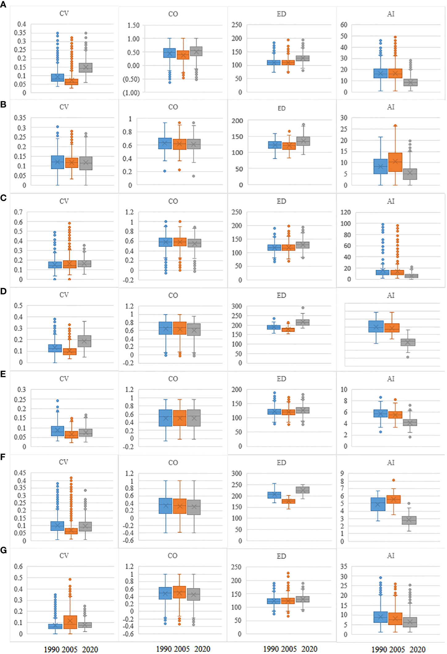
Figure 3 Values of CV, CO, ED, and AI in 1990, 2005, and 2020 for seven forest PAs. Lines in boxes represent medians, and box ends represent quartiles; whiskers mark the 95th percentiles, and circles represent outliers. Box width is proportional to the square root of the number of data points in each category. CV, spectral alpha diversity; CO, neighboring correlation; ED, spatial distance; AI, aggregation index; PAs, protected areas. (A) hz; (B) kns; (C) qls; (D) wl; (E) slj; (F) phs; (G) hls.

From low to high latitudinal gradient, CV values showed a significant v-curve (r² = 0.22), ED significantly (r² = 0.33) decreased, and AI (r² = 0.90) significantly increased (Figure 4). In turn, CO exhibited the least change. When annual precipitation increased from 900 to 1,900 mm, the values of CV increased significantly (r² = 0.33), and AI decreased significantly (r² = 0.23), whereas no significant (r² = 0.18) increase in ED (r² = 0.18) was observed.

FIGURE 4

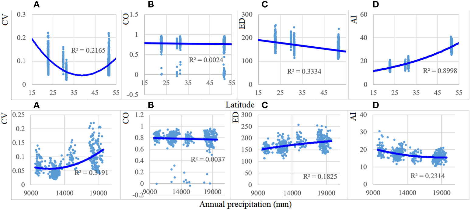
Figure 4 Patterns of CV, CO, ED, and AI with latitude and annual precipitation (×0.1 mm) gradients in 1990, 2005, and 2020. Forest spectral parameters and the environmental variables demonstrated a significant (p < 0.001) association, except those of CO. CV, spectral alpha diversity; CO, neighboring correlation; ED, spatial distance; AI, aggregation index. (A) CV; (B) CO; (C) ED; (D) AI.

3.2 Identification of key influential factors

Among the 12 models, the chi‐squared automatic interaction detector (CHAID) model yielded the most accurate predictions for all response variables across the seven PAs under study (average R² = 0.66), generalized linear modeling (GLM) (average R² = 0.61), and artificial neural network (ANN) (average R² = 0.56) (Figure 5). CHAID is based on multi‐way splits and adjusted significance testing (Bonferroni testing, p < 0.05). In every step, the predictor variable with the strongest interaction with the dependent variable was selected for the split. Default values of 100 iterations were used, with a minimum change of 0.05 in the expected cell frequencies. Our CHAID model yielded an out-of-sample predictive accuracy of 78%–98%. Therefore, five key influential climate variables were extracted based on the best model for each PA.

FIGURE 5

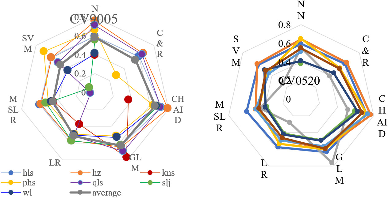
Figure 5 Model selection for regional vegetation spectral variation responses under climate change for core zones in seven protected forest areas. Vegetation spectral responses include differences between 1990–2005 (CV9005) (Left) and 2005–2020 (CV0520) (Right). Seven predictive models are shown and ranked by R2 and RMSE. ANN, artificial neural network; C&R, classification and regression tree analysis; CHAID, chi-squared automatic interaction detector; GLM, generalized linear model; LR, linear regression; MSLR, multiple stepwise linear regression; SVM, support vector machine.

Nearly 10 climate variables (Figure 5) emerged as important in the overall models, explaining 89.82% of the variation in the response matrix of spectral CV between 1990 and 2005 and 87.22% of the variation between 2005 and 2020. Both cumulative temperature values of ≥5°C and ≥10°C were important in these models, particularly in April, June, September, and October (T₁₀-6, T₅-04, T₁₀-04, T₁₀-09, and T₅-10), as was the average temperature in March and November (m03 and m11). Of all 140 selected climate variables in the 168 models, 27.86% were accounted for.

The most influential climatic factors also varied from low to high latitudinal gradients (Figure 6). For boreal forests (hz), the highest temperature in December contributed the most to the variation in the value of spectral CV (IV > 0.29). Cumulative and lowest temperatures in April (spring) were among the top predictors (IVs > 0.14) of changes in spectral CV in temperate forests (qls). The lowest temperature in winter was the key factor for changes in the spectral CV in subtropical forests (slj and phs). In the case of rainforests (hls), the key climatic factors were the highest and lowest temperatures in winter and cumulative temperatures in the spring and autumn (Figure 6).

FIGURE 6

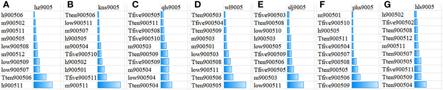
Figure 6 The 10 key climate variables that contributed the most to the variation in regional spectral CV from 1990 to 2005. m, mean temperature; h, highest temperature; low, lowest temperature; 01–12 indicate January to December; Tfive, cumulative temperature of ≥5°C; Tten, cumulative temperature of ≥10°C; 900502 indicates the difference in February between 1990s (1980–1990) and 2005s (1995–2005). (A) hz; (B) kns; (C) qls; (D) wl; (E) slj; (F) phs; (G) hls.

3.3 RDA ordination: relationships among key climate variables

As per RDA ordination, the two axes explained 14.0% of the vegetation variation in the PA of hz, 18.55% of qls, 31.11% of wl, 13.49% of slj, 64.48% of phs, and 25.39% of hls (Figure 7). In PAs with cold temperate conditions, CV values were negatively related to AI, low08 (the lowest temperature in August, the following is same), and h11 and positively related to m05 and m012. The performances of kns and qls were similar in that CV and CO values were positively associated. With respect to wl, T₁₀-5 and T₁₀-6 were negatively correlated with the CV. In sjl, low11 was positively and negatively correlated with CV and m03, respectively. Lastly, in the case of tropical and subtropical climate PAs (phs and hls), AI was negatively related to CV and differed from the values obtained in the other PAs.

FIGURE 7

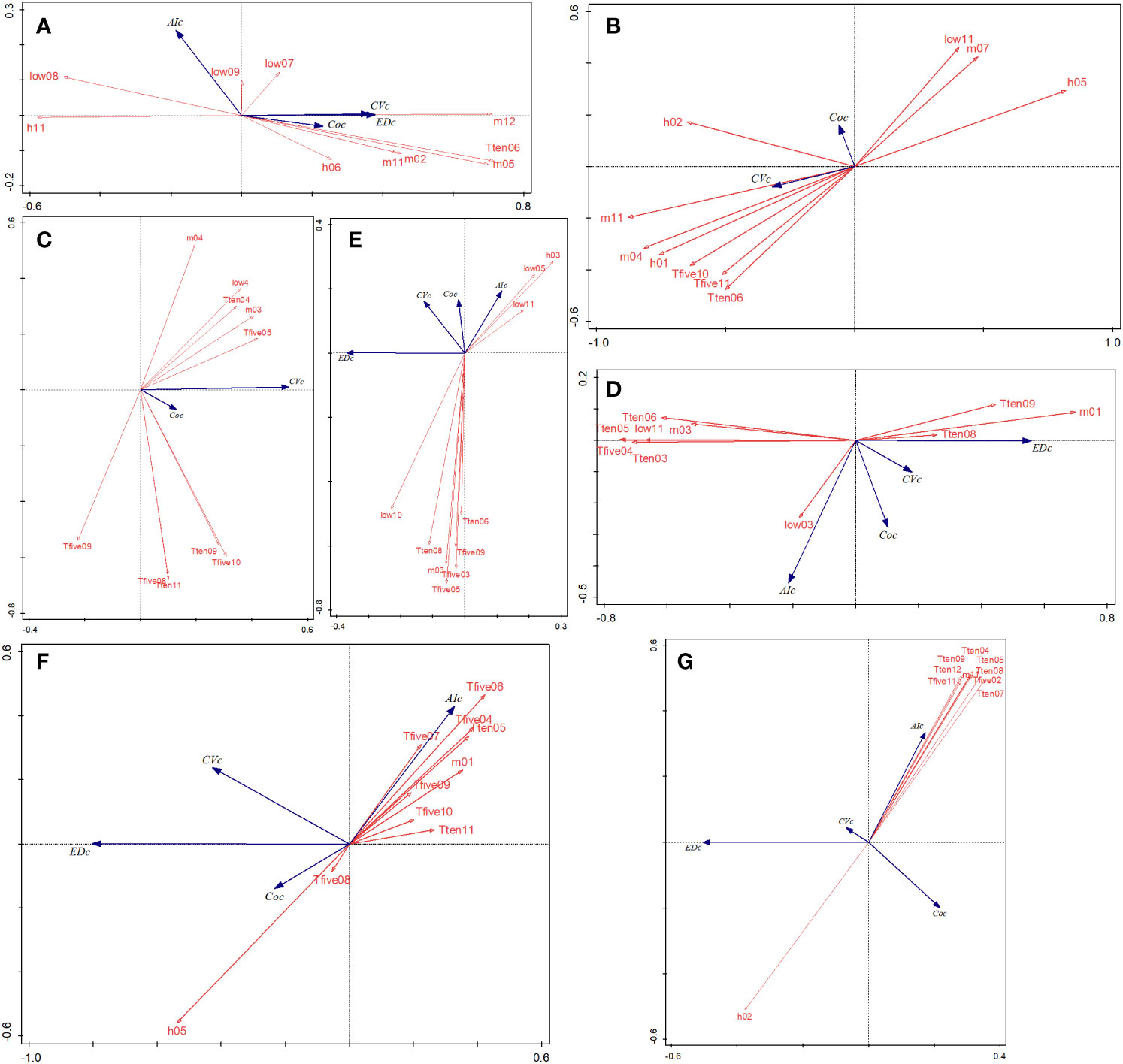
Figure 7 RDA ordinations between the regional spectral CV, ED, AI, CO, and environmental variables in seven forest PAs (A–G). EDc, Euclidean distance (m); Coc, neighboring correlation; m, average temperature during a period (×0.1°C; low, lowest temperature during a period; h, highest temperature during a period; T5, cumulative temperature ≥ 5°C during a period; T10, cumulative temperature ≥10°C during a period). RDA, redundancy analysis; CV, spectral alpha diversity; ED, spatial distance; AI, aggregation index; CO, neighboring correlation; PAs, protected areas.

3.4 Variation partitioning

Interestingly, spatial distance metrics (b; ED and AI) explained most (>10%) of the regional spectral variation of CV values in all seven PAs (Figure 8), and climate variables (a) explained a negligible proportion of CV variation (major in 0%–5%). Moreover, a greater proportion of the CV variation was explained by distance metrics (23.8%) in cold climate areas than in other areas. On average, the portion of neighbor correlation (c; Cor, 3.7%) was larger than that of climate variables (a; 2.3%). In tropical areas (hls), the interaction between climatic conditions and neighboring correlations (f) showed 10.8% of the spectral CV variation, whereas in cold areas (hz), this interaction accounted for only 0.6%.

FIGURE 8

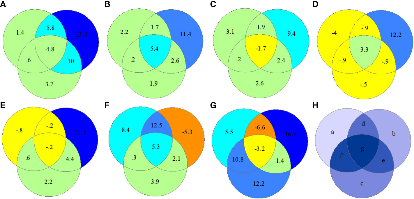
Figure 8 RDA ordination-based regional spectral CV variation partitioning in seven protected forest areas by selecting “Var-part-3groups-conditional-effects-tested.” a, climate (ten climate variables selected); b, spatial distance (ED and AI); c, neighbor interaction (CO); d = a + b, e = b + c, f = a + c, and g = d + e + f. (A) hz; (B) kns; (C) qls; (D) wl; (E) slj; (F) phs; (G) hls; (H) components of variation partitioning. RDA, redundancy analysis; CV, spectral alpha diversity; ED, spatial distance; AI, aggregation index; CO, neighboring correlation.

4 Discussion

This study is the first attempt to link climate change, neighboring interactions, and spatial distance to species richness and evenness. Using high-accuracy modern machine learning models, we identified the key influencing factors that contributed to the variation in spectral diversity on a large scale using 27 climatic variables. Furthermore, we evaluated the contribution of climate, neighboring interactions, and spatial distance to the variation in spectral CV across forest types.

Consistent with previous studies (Zhang et al., 2017), our results indicated that spectral diversity has increased with climate warming. A recent study found that species richness increased on mountain summits in boreal-temperate forests in Europe (Pauli et al., 2012). Over 30 years of succession, species richness and phylogenetic diversity of plantation trees have increased monotonically (Yu et al., 2019). An increase in spectral species richness is closely associated with an increase in the NDVI, effective cumulative temperature, and seasonal variation in moisture availability (Harrison et al., 2015). In heterogeneous grasslands in California (USA), livestock grazing, fire, succession, nitrogen deposition, and exotic species did not contribute to fluctuations in plant diversity (Harrison et al., 2015). In this study, monthly cumulative temperature, rather than annual average temperature, contributed the most to the increase in spectral CV from 1990 to 2020.

We found that neighboring interactions and plant–plant spatial distance increased with increasing species diversity, presumably due to an increase in tree productivity and tree abundance resulting from ecological complementarity. A previously published global meta-analysis demonstrated that diversity effects are prevalent in the most productive environments, whereas abundance effects became dominant under the most limiting conditions (Madrigal-González et al., 2020). Therefore, a higher abundance will definitely affect plant–plant interactions (i.e., neighboring interactions), and the consequences of this may be either positive or negative, depending on species traits, economics, and environmental conditions (Madrigal-González et al., 2020). A meta-analysis showed that larger positive effects favored sapling emergence and survival, whereas smaller negative effects act on plant growth and density (Gómez-Aparicio, 2009). The life form of the interacting species largely influences the outcome of the interaction; for example, herbaceous plants have strong negative effects, especially on other herbaceous species, whereas shrubs have strong supportive effects, especially on trees (Gómez-Aparicio, 2009). Semiarid and tropical ecosystems, but particularly temperate ecosystems, show more positive neighbor effects than wetlands (Gómez-Aparicio, 2009). Biotic interactions are thought to be relatively more important in shaping biodiversity at tropical than at temperate latitudes (Roslin et al., 2017). Ignoring biotic interactions affects the estimate of climatic niche limits that determine the responses of plant diversity to climate change in models (Newbold et al., 2020). The results of the current study underscore the need to include biotic interactions in climate change modeling.

Neighboring species may demonstrate strong positive or negative correlations. However, when both types of correlation exist, the total neighboring interaction in the region may become null or weak, given that positive and negative values counteract each other (Dray et al., 2012). Weak or null values of neighboring interactions may result when both positive and negative correlations shape species spatial distributions (Wagner, 2013; Biswas et al., 2016). In the present study, warming on a regional scale increased plant species richness (spectral CV), creating a stronger spatial correlation between neighboring species, whereas competition on a plant–plant scale created a negative spatial correlation (Biswas et al., 2017). Although neighboring interactions were weak, they still highly contributed to variation in plant species diversity (spectral CV) in our study.

Considering these results, it is reasonable to expect that stronger neighboring interactions will enhance plant–plant competition, thereby producing a negative effect on intraspecific associations. Conclusively, only species distributed over large distances will survive. Therefore, climate warming leads to a large plant–plant distance. Hypotheses 2 and 3 were confirmed by our data. Specifically, we found that the spatial distance between the same spectral species increased with increasing spectral CV under climate change. The spatial patterns of communities are shaped by environmental filtering and biological competition. Environmental filtering produces a spatially aggregated pattern, whereas competition produces a spatially segregated pattern (He & Biswas, 2019). Possibly, intraspecies competition played a stronger role than environmental filtering in structuring the communities studied from 1990 to 2020, likely because the soil properties, landforms, and slope remained unchanged during this period, whereas plant diversity (spectral CV) increased. To a certain extent, higher plant abundance and species numbers might have confounded the positive effects of climate warming at a local scale. Moreover, our results confirmed that the contribution of plant–plant distance to species diversity was higher than that of climate variables for all forest types (hypothesis 1). Consistent with these findings, a previously published field experiment has shown that biotic interactions have a strong effect on plant fitness and eventually override the effects of climate (Tomiolo et al., 2015).

The patterns of spectral metrics in response to climate change were the same as those in the field survey. Consequently, we determined that spectral metrics are reliable proxy measures of plant species parameters. Several dissimilarity measurements have been introduced to quantify the overall heterogeneity in plant species composition on a few or multiple sites. However, pairwise dissimilarities do not account for patterns of co-occurrence at more than two sites (Baselga, 2013). Consequently, the average of the pairwise dissimilarities may not accurately reflect the overall compositional heterogeneity at multiple sites (Baselga, 2013). Within a highly diverse plant community, many plant species lived together or were associated with higher stem abundance. In remote sensing images, the former demonstrates a cluster with high heterogeneity, while the latter demonstrates similar neighboring pixels. A dataset based on remote sensing is reliable for analyzing both the spectral diversity and spatial patterns of plant species in forests.

In the current study, we found that geophysical factors including soil pH and clay content tended to have higher effects on tree species diversity. Although climate is changing rapidly, geophysical factors are relatively fixed and are not likely to change significantly over the timescales considered in this analysis. Consequently, geophysical variables were not included in the models. In addition, evolutionary and biogeographic histories, including past diversification processes and environmental changes, influence the distribution of tree diversity, and such factors should be considered in future studies on the spatial patterns of plant diversity.

5 Conclusions

Our results indicated that climate warming has increased species diversity, which in turn has increased neighboring interactions, ultimately leading to a longer plant–plant distance. However, we found that climate change contributed less to species diversity than neighboring interactions and spatial distance. Conclusively, we did not detect a significant change in the overall neighboring correlation on a regional scale under climate warming, although we did observe an increase in the spatial distance across spectral species. In future studies, the relevant biotic and abiotic factors should be quantified, and an assessment of the relative contribution of abiotic factors to the spatial pattern of species diversity should be performed. The general effects of neighboring interactions on plant diversity should be considered at the global scale, considering all vegetation types under the conditions of ongoing climate change.

Data availability statement

The original contributions presented in the study are included in the article/Supplementary Material. Further inquiries can be directed to the corresponding author.

Author contributions

YP devised the project and developed the research questions and study design. NP and JX processed and analyzed data. All authors contributed to the manuscript writing and editing. All authors contributed to the article and approved the submitted version.

Funding

This research was funded by the General Program of the National Natural Science Foundation of China (32271555), the Top Discipline and First-class University Construction Project (ydzxxk201618) of Minzu University of China, and Special Project of Strategic Leading Science and Technology of Chinese Academy of Sciences (No: XDA 19030104).

Conflict of interest

The authors declare that the research was conducted in the absence of any commercial or financial relationships that could be construed as a potential conflict of interest.

Publisher’s note

All claims expressed in this article are solely those of the authors and do not necessarily represent those of their affiliated organizations, or those of the publisher, the editors and the reviewers. Any product that may be evaluated in this article, or claim that may be made by its manufacturer, is not guaranteed or endorsed by the publisher.

Supplementary material

The Supplementary Material for this article can be found online at: https://www.frontiersin.org/articles/10.3389/fevo.2023.1137111/full#supplementary-material

References

Aguirre-Gutiérrez J., Oliveras I., Rifai S., Fauset S., Adu-Bredu S., Affum-Baffoe K., et al. (2019). Drier tropical forests are susceptible to functional changes in response to a long-term drought. Ecol. Lett. 22, 855–865. doi: 10.1111/ele.13243

PubMed Abstract | CrossRef Full Text | Google Scholar

Baselga A. (2013). Multiple site dissimilarity quantifies compositional heterogeneity among several sites, while average pairwise dissimilarity may be misleading. Ecography 36 (2), 124–128. doi: 10.1111/j.1600-0587.2012.00124.x

CrossRef Full Text | Google Scholar

Biswas S. R., Macdonald R. L., Chen H. (2017). Disturbance increases negative spatial autocorrelation in species diversity. Landscape Ecol. 32 (4), 823–834. doi: 10.1007/s10980-017-0488-9

CrossRef Full Text | Google Scholar

Biswas S. R., Mallik A. U., Braithwaite N. T., Wagner H. H. (2016). A conceptual framework for the spatial analysis of functional trait diversity. Oikos 125 (2), 192–200. doi: 10.1111/oik.02277

CrossRef Full Text | Google Scholar

Boutin M., Corcket M., Alard D., Villar L., Jiménez J. J., Blaix C., et al. (2017). Nitrogen deposition and climate change have increased vascular plant species richness and altered the composition of grazed subalpine grasslands. J. Ecol. 105 (5), 1199–1209. doi: 10.1111/1365-2745.12743

CrossRef Full Text | Google Scholar

Dray S., Pelissier R., Couteron P., Fortin M. J., Legendre P., Peres-Neto P.R., et al. (2012). Community ecology in the age of multivariate multiscale spatial analysis. Ecol. Monogr. 82 (3), 257–275. doi: 10.1890/11-1183.1

CrossRef Full Text | Google Scholar

Duro D. C., Girard J., King D. J., Fahrig L., Mitchell S., Lindsay K., et al. (2014). Predicting species diversity in agricultural environments using Landsat TM imagery. Remote Sens. Environ. 144, 214–225.

Google Scholar

Engler R., Randin C. F., Vittoz P., Czáka T., Beniston M., Zimmermann N. E., et al. (2009). Predicting future distributions of mountain plants under climate change: does dispersal capacity matter? Ecography 32, 34–45. doi: 10.1111/j.1600-0587.2009.05789.x

CrossRef Full Text | Google Scholar

Fassnacht F., Hartig F., Latifi H., Berger C., Hernández J., Corvalán P., et al (2014). Importance of sample size, data type and prediction method for remote sensing-based estimations of aboveground forest biomass. Remote Sens. Environ. 154, 102–114. doi: 10.1016/j.rse.2014.07.028

CrossRef Full Text | Google Scholar

Gómez-Aparicio L. (2009). The role of plant interactions in the restoration of degraded ecosystems: a meta-analysis across life-forms and ecosystems. J. Ecol. 97, 1202–1214. doi: 10.1111/j.1365-2745.2009.01573.x

CrossRef Full Text | Google Scholar

Hall-Beyer M. (2017). Practical guidelines for choosing GLCM textures to use in landscape classification tasks over a range of moderate spatial scales. Int. J. Remote Sens. 38, 1312–1338.

Google Scholar

Harrison S. P., Gornish S. E., Copeland S. (2015). Climate-driven diversity loss in a grassland. Proc. Natl. Acad. Sci. 112 (28), 8672–8677. doi: 10.1073/pnas.1502074112

CrossRef Full Text | Google Scholar

Harrison S., Spasojevic M. J., Li D. (2020). Climate and plant community diversity in space and time. Proc. Natl. Acad. Sci. U.S.A. 117 (9), 4464–4470. doi: 10.1073/pnas.1921724117

PubMed Abstract | CrossRef Full Text | Google Scholar

He D., Biswas S. R. (2019). Negative relationship between interspecies spatial association and trait dissimilarity. Oikos 128, 659–667. doi: 10.1111/oik.05876

CrossRef Full Text | Google Scholar

He H. S., DeZonia B. E., Mladenoff D. J. (2000). An aggregation index (AI) to quantify spatial patterns of landscapes. Landscape Ecol. 15, 591–601. doi: 10.1023/A:1008102521322

CrossRef Full Text | Google Scholar

He N., Wen D., Zhu J., Tang X., Xu L., Zhang L., et al. (2017). Vegetation carbon sequestration in Chinese forests from 2010 to 2050. Global Change Biol. 23, 1575–1584. doi: 10.1111/gcb.13479

CrossRef Full Text | Google Scholar

Hernández-Stefanoni J. L., Gallardo-Cruz J. A., Meave J. A., Rocchini D., Bello-Pineda J., López-Martínez J. O. (2012). Modeling α-and β-diversity in a tropical forest from remotely sensed and spatial data. Int. J. Appl. Earth Observ. Geoinf. 19, 359–368. doi: 10.1016/j.jag.2012.04.002

CrossRef Full Text | Google Scholar

Karl T. R., Arguez A., Huang B., Lawrimore J. H., McMahon J. R., Menne M. J., et al. (2015). CLIMATE CHANGE. possible artifacts of data biases in the recent global surface warming hiatus. Science 348 (6242), 1469–1472. doi: 10.1126/science.aaa5632

PubMed Abstract | CrossRef Full Text | Google Scholar

Kelsey K. C., Neff J. C. (2014). Estimates of aboveground biomass from texture analysis of Landsat imagery. Remote Sens. 6 (7), 6407–6422. doi: 10.3390/rs6076407

CrossRef Full Text | Google Scholar

Kreft H., Jetz W. (2007). Global patterns and determinants of vascular plant diversity. Proc. Natl. Acad. Sci. U.S.A. 104, 5925–5930. doi: 10.1073/pnas.0608361104

PubMed Abstract | CrossRef Full Text | Google Scholar

Lepš J., Šmilauer P. (2003). Multivariate analysis of ecological data using CANOCO (Cambridge, UK: Cambridge University Press).

Google Scholar

Levin N., Shmida A., Levanoni O., Tamari H., Kark S. (2007). Predicting mountain plant richness and rarity from space using satellite-derived vegetation indices: predicting mountain biodiversity from space. Divers. Distrib. 13 (6), 692–703. doi: 10.1111/j.1472-4642.2007.00372.x

CrossRef Full Text | Google Scholar

Li X. R., Jia R. L., Zhang Z. S., Zhang P, Hui R. (2018). Hydrological response of biological soil crusts to global warming: a ten-year simulative study. Global Change Biol. 24 (10), 4960–4971. doi: 10.1111/gcb.14378

CrossRef Full Text | Google Scholar

Madonsela S., Cho M. A., Ramoelo A., Mutanga O. (2017). Remote sensing of species diversity using Landsat 8 spectral variables. ISPRS J. Photogram. Remote Sens. 133, 116–127. doi: 10.1016/j.isprsjprs.2017.10.008

CrossRef Full Text | Google Scholar

Madrigal-González J., Calatayud J., Ballesteros-Canovas J. A., Escudero A., Stoffel M. (2020). Climate reverses directionality in the richness-abundance relationship across the world's main forest biomes. Nat. Commun. 11 (1), 5635. doi: 10.1038/s41467-020-19460-y

PubMed Abstract | CrossRef Full Text | Google Scholar

Matos P., Geiser L., Hardman A., Glavich D., Pinho P., Nunes A., et al. (2017). Tracking global change using lichen diversity: towards a global-scale ecological indicator. Methods Ecol. Evol. 8, 788–798. doi: 10.1111/2041-210X.12712

CrossRef Full Text | Google Scholar

Neves D. M., Dexter K.G., Baker T. R., de Souza F. C., Oliveira-Filho A.T., Queiroz L.P., et al. (2020). Evolutionary diversity in tropical tree communities peaks at intermediate precipitation. Sci. Rep. 10, 1188. doi: 10.1038/s41598-019-55621-w

PubMed Abstract | CrossRef Full Text | Google Scholar

Newbold T., Oppenheimer P., Etard A., Williams J. J. (2020). Tropical and mediterranean biodiversity is disproportionately sensitive to land-use and climate change. Nat. Ecol. Evol. 4, 1630–1638. doi: 10.1038/s41559-020-01303-0

PubMed Abstract | CrossRef Full Text | Google Scholar

Pauli H., Gottfried M., Dullinger S., Abdaladze O., Akhalkatsi M., Alonso J. L. B., et al. (2012). Recent plant diversity changes on Europe’s mountain summits. Science 336 (6079), 353–355. doi: 10.1126/science.1219033

PubMed Abstract | CrossRef Full Text | Google Scholar

Peng Y., Fan M., Bai L., Sang W., Feng J., Zhao Z., et al. (2019). Identification of the best hyperspectral indices in estimating plant species richness in sandy grasslands. Remote Sens. 11, 588. doi: 10.3390/rs11050588

CrossRef Full Text | Google Scholar

Peñuelas J., Sardans J., Estiarte M., Ogaya R., Carnicer J., Coll M., et al. (2013). Evidence of current impact of climate change on life: a walk from genes to the biosphere. Glob. Change Biol. 19, 2303–2338. doi: 10.1111/gcb.12143

CrossRef Full Text | Google Scholar

Réjou-Méchain M., Mortier F., Bastin J. F., Cornu G., Barbier N., Bayol N., et al. (2021). Unveiling African rainforest composition and vulnerability to global change. Nature 593 (7857), 90–94. doi: 10.1038/s41586-021-03483-6

PubMed Abstract | CrossRef Full Text | Google Scholar

Ricklefs R. E., He F. (2016). Region effects influence local tree species diversity. Proc. Natl. Acad. Sci. United States America 113, 674–679.

Google Scholar

Rocchini D. (2007). Effects of spatial and spectral resolution in estimating ecosystem α-diversity by satellite imagery. Remote Sens. Environ. 111, 423–434. doi: 10.1016/j.rse.2007.03.018

CrossRef Full Text | Google Scholar

Roslin T., Hardwick B, Novotny V, Petry WK, Andrew NR, Asmus A, et al. (2017). Higher predation risk for insect prey at low latitudes and elevations. Science 356, 742–744. doi: 10.1126/science.aaj1631

PubMed Abstract | CrossRef Full Text | Google Scholar

Sullivan M. J. P., Lewis S. L., Affum-Baffoe K., Castilho C., Costa F., Sanchez A. C., et al. (2020). Long-term thermal sensitivity of Earth’s tropical forests. Science 368, 869–874. doi: 10.1126/science.aaw7578

PubMed Abstract | CrossRef Full Text | Google Scholar

Tomiolo S., van der Putten W. H., Tielbörger K. (2015). Separating the role of biotic interactions and climate in determining adaptive response of plants to climate change. Ecology 96, 1298–1308. doi: 10.1890/14-1445.1

PubMed Abstract | CrossRef Full Text | Google Scholar

Wagner H. H. (2013). Rethinking the linear regression model for spatial ecological data. Ecology 94 (11), 2381–2391. doi: 10.1890/12-1899.1

PubMed Abstract | CrossRef Full Text | Google Scholar

Wallis C. I. B., Brehm G., Donoso D. A., Fiedler K., Homeier J., Paulsch D., et al (2017). Remote sensing improves prediction of tropical montane species diversity but performance differs among taxa. Ecol. Indicators 83, 538–549.

Google Scholar

Wang C., Yang J., Zhang Q. (2010). Soil respiration in six temperate forests in China. Global Change Biol. 12 (11), 2103–2114. doi: 10.1111/j.1365-2486.2006.01234.x

CrossRef Full Text | Google Scholar

Yu Q., Rao X., Ouyang S., Xu Y., Hanif A., Ni Z., et al. (2019). Changes in taxonomic and phylogenetic dissimilarity among four subtropical forest communities during 30 years of restoration. For. Ecol. Manage. 432, 983–1001. doi: 10.1016/j.foreco.2018.10.033

CrossRef Full Text | Google Scholar

Zhang J., Nielsen S. E., Chen Y., Georges D., Qin Y., Wang S., et al. (2017). Extinction risk of North American seed plants elevated by climate and land-use change. J. Appl. Ecol. 54, 303–312. doi: 10.1111/1365-2664.12701

CrossRef Full Text | Google Scholar

Zwiener V. P., Lira-Noriega A., Grady C. J., Padial A. A., Vitule J. R. S. (2018). Climate change as a driver of biotic homogenization of woody plants in the Atlantic Forest. Global Ecol. Biogeogr. 27, 298–309. doi: 10.1111/geb.12695

CrossRef Full Text | Google Scholar