 Becky Tang
 Renata P. Kamakura
 David T. Barnett
 James S. Clark
95% of researchers rate our articles as excellent or good
Learn more about the work of our research integrity team to safeguard the quality of each article we publish.
Find out more
HYPOTHESIS AND THEORY article
Front. Ecol. Evol. , 04 April 2023
Sec. Models in Ecology and Evolution
Volume 11 - 2023 | https://doi.org/10.3389/fevo.2023.1114569
This article is part of the Research Topic Modeling, Data Handling, and Analysis: Practical and Fundamental Consequences in Ecology and Evolution View all 9 articles
In order to learn about broad scale ecological patterns, data from large-scale surveys must allow us to either estimate the correlations between the environment and an outcome and/or accurately predict ecological patterns. An important part of data collection is the sampling effort used to collect observations, which we decompose into two quantities: the number of observations or plots (n) and the per-observation/plot effort (E; e.g., area per plot). If we want to understand the relationships between predictors and a response variable, then lower model parameter uncertainty is desirable. If the goal is to predict a response variable, then lower prediction error is preferable. We aim to learn if and when aggregating data can help attain these goals. We find that a small sample size coupled with large observation effort coupled (few large) can yield better predictions when compared to a large number of observations with low observation effort (many small). We also show that the combination of the two values (n and E), rather than one alone, has an impact on parameter uncertainty. In an application to Forest Inventory and Analysis (FIA) data, we model the tree density of selected species at various amounts of aggregation using linear regression in order to compare the findings from simulated data to real data. The application supports the theoretical findings that increasing observational effort through aggregation can lead to improved predictions, conditional on the thoughtful aggregation of the observational plots. In particular, aggregations over extremely large and variable covariate space may lead to poor prediction and high parameter uncertainty. Analyses of large-range data can improve with aggregation, with implications for both model evaluation and sampling design: testing model prediction accuracy without an underlying knowledge of the datasets and the scale at which predictor variables operate can obscure meaningful results.
In order to understand and predict ecological processes, researchers often draw on data from regional sampling networks. However, when using these data, it is common to combine data sets or ask questions different from those for which the sampling was originally designed (Tinkham et al., 2018); thus, the analysis may need to adjust for differences in scale and focus between the sampling design and analysis goals. Similarly, investigators and institutions confront several design decisions with implications for further data analysis when creating regional sampling networks (Gregoire and Valentine, 2007). including and especially the size and number of plots to use to sufficiently sample the underlying variation relevant to ecological or bio-geographic patterns of interest (Zeide, 1980; Wang et al., 2001, 2008).
As part of effectively designing new studies or asking new questions of existing datasets, we must better understand the impact of a critical component of the process: the total sampling effort used to collect observations. In particular, we seek to learn how exploratory and predictive modeling goals are affected by the total sampling effort used to collect the data. To this end, we decompose the sampling effort of a given study into two quantities: the number of observations (n) and the effort per observation (E). We demonstrate that, when looking at broad ecological patterns, analyses and potentially sampling design need to balance the trade-offs of using/collecting data from few, intensely-sampled locations vs. a larger number of locations sampled with less intensity. Throughout this paper, we refer to this trade-off of few, large observation efforts vs. many, small observation efforts as FLvMS.
FLvMS decisions broadly depend upon the geographic scale of the processes and patterns that the network aims to monitor or understand. When we consider scale, we mean questions of geographic focus, for example, the size of a geographic region being sampled or the area over which the variation driven by an ecological process operates. Large observation plots (e.g., ForestGeo Anderson-Teixeira et al., 2015) can provide detailed information about habitats and communities, such as increasing probability of capturing rare events (e.g., Barnett and Stohlgren, 2003). This benefit comes with the cost of observing only a limited set of potential sites or habitats. Alternatively, numerous small plots can extend the range of observed ecological variation, but with limited information per plot. Current monitoring designs do attempt to balance information at local and regional scales under the inevitable constraint of resources. While ideas related to FLvMS are mentioned in recent efforts to guide prediction from monitoring networks (Zeide, 1980; Wang et al., 2001, 2008; Wintle et al., 2010; Yim et al., 2015; McRoberts et al., 2018), there is limited work looking specifically at the impacts of FLvMS for statistical regression modeling, as we elaborate below (Dietze et al., 2018).
We find that FLvMS can have practical implications for the quality of ecological insights gained from data. When fitting models, studies tend to focus on the following aspects of the model: its explanatory ability and its utility for prediction. Explanatory modeling focuses on understanding how a set of predictor variables are associated with or affect a response variable, often through an assumed parametric relationship (e.g., regression models). In this context, low uncertainty for the parameters estimates is desirable in order to obtain statistical conclusions for hypotheses and theory. The goal of predictive modeling is to obtain precise predictions for new or future observations, which can be important for decision-making and policy recommendations (Iwamura et al., 2020; Malik et al., 2021). Predictive power is typically assessed using metrics (e.g., root mean squared error) computed from a held-out validation set, where improved metrics imply improved prediction accuracy on that validation set. A model that makes poor predictions might still advance understanding of why or how ecological phenomena occur if it provides parameter estimates with low uncertainty. Conversely, parameter estimates with low uncertainty do not necessarily make for good predictions, especially in complex systems (Lo et al., 2015). The distinction between the two goals has practical implications for sampling design in networks focused on broad-scale ecological and biophysical patterns (Shmueli, 2010). In this work, we explore how design decisions involving FLvMS can affect parameter estimates and predictions in different ways. We do not claim to address all relevant factors related to FLvMS for design (with the notable omission of sampling costs and crew time/costs), but instead address a gap in statistical evaluation often seen in discussions around FLvMS.
FLvMS is also a consideration beyond the design stage; when using previously collected data, analyses can benefit from combining or aggregating observations in order to reduce noise depending on the spatial distribution pattern of the process(es) of interest. Observations may be aggregated in space (Iverson and Prasad, 1998), time (Crewe et al., 2016), or environmental conditions (Andelman and Willig, 2004; Zhu et al., 2014; Schliep et al., 2016). Compositing multiple observations taken at several microsites or sub-plots within a single site is a type of aggregation that can also reduce noise, depending on the design of subplots (e.g., soil samples, Singh et al., 2020). Here, we describe the original plot/observation as the original sampling unit. When observations are aggregated together, we refer to these modified observations as having different units of analysis for modeling (e.g., 10 observations aggregated into a single quantity has a unit of analysis of 10; Neuendorf, 2021). However, the potential benefits of increased effort per observation, aggregated/composited unit of analysis, may be offset by the undesirable effect of masking processes operating at fine spatio-temporal scales (Rossi et al., 1992; Jelinski and Wu, 1996; Liebhold and Gurevitch, 2002; Maas-Hebner et al., 2015). Thus, the FLvMS trade-off should be a ubiquitous design consideration for both observational studies and resulting analyses.
We provide a framework for network design and data aggregation that integrates FLvMS to demonstrate several insights, (i) low uncertainty for predictions depends on large effort per observation (E), whereas low uncertainty for parameter estimates depends on large total sample effort (effort per observation × number of observations, or S = nE), (ii) prediction accuracy usually improves with data aggregation, whereas parameter uncertainty does not, (iii) poor predictions that come from designs based on small plots may be rehabilitated by aggregating the predictions, and (iv) models can have high predictive accuracy yet non-informative parameter estimates. We start with theory and simulations, followed by an application to Forest Inventory and Analysis (FIA) data that further explores the impacts of aggregation. Material provided in the Supplement are referred to with an “S.”
Understanding the divergent effects of FLvMS for parameters and predictions requires the concepts of observation effort and sample effort. A sample consists of n observations. The fundamental FLvMS trade-off concerns the distribution of effort over the n observations. Consider a response yi at location i observed with an associated observation effort Ei. Total sampling effort is the summed observation effort,
Terms related to FLvMS are defined in Table 1. For fixed S, a design based on many small plots involves large n and low Ei. Where observation effort is constant (Ei = E) we see this trade-off directly: S = nE.
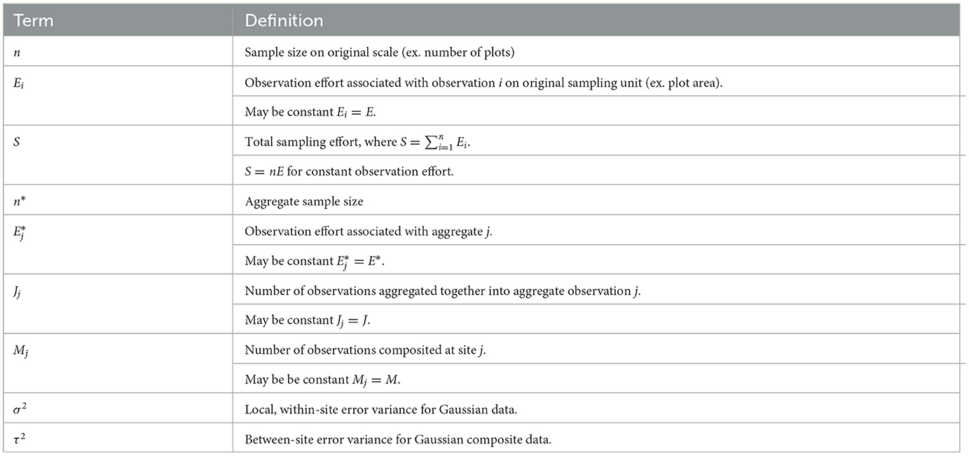
Table 1. Terms and definitions related to few-large vs. many-small and aggregation concepts.
In networks where plots are not clustered, aggregating observations within the existing network reduces the effective sample size (↓n), while increasing the effective observation effort (↑E), but we demonstrate that it does not change the sample effort, S. We use the symbol * to denote quantities associated with aggregation: a sample of n = 10, 000 plots, each with effort E = 1m2, could be aggregated to groups of J = 10 plots with aggregate sample size n* = 1, 000 and aggregate effort E* = 10m2. For (discrete) count data, an aggregate observation j has response and aggregate effort , where Aj holds the indices of the original observations associated with aggregate j. Summing over n* yields S. A simple graphic of this aggregation design is shown in Figure 1. Where observation effort is constant (ignoring any fixed costs associated with each plot, e.g., travel), the total sample effort S is unchanged by aggregation, i.e., S = nE = n*E*. For heterogeneous effort,
In this paper, we view the concept of effort applied to continuous responses involves averages rather than sums. We imagine the practice of averaging water or soil samples to reduce the noise and obtain more precise measurements of concentrations or mineralization rates. We note that averaging is not appropriate for aggregating count data, as the average of discrete counts might no longer be discrete. So for continuous y, where Jj = |Aj|.
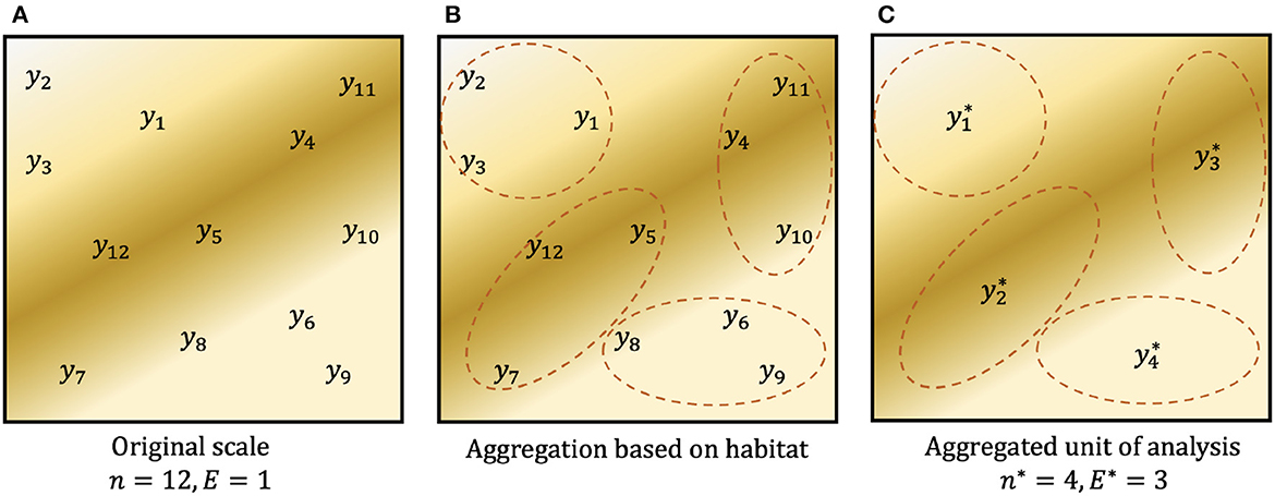
Figure 1. Example graphic of aggregating count data. (A) Observed counts y1, …, y12 at single plots (E = 1) within a spatial region. Background color denotes the spatial distribution of an environmental predictor such as habitat. (B) Possible aggregation of the original data based on habitat. (C) Data aggregated to a new unit of analysis, where , and similarly for the other three aggregated observations. On this unit of analysis, there are n* = 4 observations, each obtained with aggregated observation effort E* = 3. In both (A, C), total sampling effort is S = 12.
Observations can be aggregated within or between plots. For example, multiple soil and water measurements from the same plot are composited to reduce noise (e.g., Singh et al., 2020). The increase in effort, represented by the composite measurement, reduces the composite variance, as we demonstrate in Section 2.2.
Because observation and sample effort are not often discussed in the context of trade offs between goals of prediction and parameter estimation, the majority of this section (Sections 2.2, 2.3) comprises analytical solutions that provide general principles based on how sample effort S is distributed between sample size n and observations effort E. We focus on the effects of n, E, and S on parameter estimation (Section 2.2) and prediction uncertainty (Section 2.3) in the context of discrete and continuous data. This section finishes with details concerning simulations (Section 3.1) and an application to the FIA monitoring network (Section 3.2).
In models for count data yi, the quantity of interest is often counts per effort CPEi = yi/Ei. For non-moving organisms (e.g., plants), effort is represented by plot area. For point counts, camera traps, and pitfall traps (e.g., vertebrates and insects), effort is observation time, and CPE is counts per unit time. In fisheries, effort may be the number of trawls and CPE is catch per trawl. As an example, consider the semi-structured, global citizen science eBird (2017) dedicated to avifauna observation. Observers report the number of bird species detected on a bird outing, where the observation duration can vary from 1 min to several hours. A statistical model for the bird counts needs to adjust for the duration of each observation, as one bird observed in 1 min is different from one bird observed over the course of 2 h. Thus, the duration of each bird outing can be viewed as observation effort (Tang et al., 2021), and CPE could be the number of birds observed in a 30 min time frame. In these cases, observation effort Ei is a known quantity that is not estimated.
Poisson regression models are often used for modeling counts yi. Observation effort Ei typically enters a Poisson model as follows: yi~Pois(Eiλ). In a generalized linear model, Ei is known as an offset for yi, as Ei is fixed and known in advance. This specification changes the parameter estimate from an intensity to a rate (per area, per time, and so forth). For simplicity, let effort be constant, so Ei = E. Then the estimate that maximizes the Poisson likelihood, or MLE, is , where ȳ is the observed sample mean. has asymptotic variance . Re-writing in the scale of interest CPEi = yi/E, the MLE and its uncertainty are
where . In other words, the estimate has units determined by observation effort E, but the uncertainty depends on sample effort S, regardless of how it is allocated between n vs. E.
Aggregation does not change this result, yielding
Thus, FLvMS by itself does not affect parameter uncertainty, which depends instead on total sample effort. However, spatial patterns may change this result (see Section 4.1, 4.2).
As for discrete counts, increasing effort has minimal impact on parameter uncertainty for a continuous response. The linear regression model with predictors held in n × p matrix X is , with Gaussian noise . Here, xi is p-vector of predictors and intercept. The estimated parameters and associated covariance are
where Vx is the covariance in predictors.
In this continuous case, it can be useful to think about residual variation as an inverse of effort. For example, consider the effect of compositing M measurements within a given site, where compositing yields one single sample from the site. Assuming independence, the variance for the composited sample reduces from σ2 to σ2/M, where σ2 is the residual variance from the linear regression model. In the sense that effort reduces error, σ2 can be likened to error with minimal effort (M = 1). Defining observation effort E = 1/σ2 allows observation effort to enter the model in the continuous case, as Equation 8 becomes
Note that in the linear regression setting, the residual variances σ2 are assumed equal across observations i, so observation effort E is similarly assumed constant across i.
Where the predictors are replaced with an overall mean μ, Equation 9 simplifies to . Where predictors are not only centered, but also standardized, they too have variance . Thus, as in the discrete case, the parameter uncertainty depends on total effort, not n alone or E alone.
Unlike discrete data where aggregated counts are sums, aggregating continuous data is done by averaging across Jj observations. In this framework, we imagine each location i has a single observation, and aggregation averages the responses across Jj unique sampling locations. Taking constant Jj = J, aggregation leads to reduced sample size n* = n/J, increased effort E* = EJ, and, if we assume for the moment independent observations, reduced variance . Letting YJ be the vector holding the aggregated responses yj, the estimated parameters and associated covariance on the aggregated unit of analysis are
where VJ is the covariance in the aggregated predictors XJ. If the covariance in predictors is unaffected by aggregation (i.e., Vx = VJ), then as in the discrete case, the uncertainty in depends on total sampling effort S and not n or E alone.
In some cases, variance in the continuous response may have two components: variance between repeated measurements at a given location i (σ2), and variance between locations (τ2). The residual variance combines within- and between- site variances: . In the geostatistical literature, σ2 is the “nugget”. When compositing M measurements within each site i, the composite response is . Composited effort increases with the number of measurements: E* = ME = M/σ2. In this setting, the covariance of the coefficients is
where . If local variance is large (σ2 >> τ2), then uncertainty scales with 1/SM, not M alone and not (unless it is small) n alone. Conversely, if local variance is small (τ2 dominates), then , and increasing sample size n does more to reduce parameter uncertainty than compositing M.
These analytical solutions illustrate the important point that networks based on large sample effort produce the most informative parameter estimates. In both discrete and continuous cases, parameter uncertainty shows the same decline with total effort S, regardless of how it is allocated between n and E.
Paradoxically, the importance of total effort S for parameter estimation, regardless of its allocation to n vs. E, does not hold for prediction. In fact, observation effort E assumes the dominant role in prediction, with n (and thus, S) only becoming important when n is small [though this can depend upon the context and underlying spatial heterogeneity, e.g., Nyyssönen and Vuokila (1963)]. We show this with simulation for the Poisson case in Section 4.1, and demonstrate the analytic results for the continuous Gaussian case here.
Interest lies in the uncertainty around a prediction ŷi for given predictors xi. For observation i, the linear regression model with intercept α and p predictors held in xi is
once again with Gaussian noise . Let the predictors xi be centered across the observations. With observation effort E = 1/σ2, this model has predictive variance.
where Vx is the variance in the predictors. Unless n is small, the second term dominates, because S = n × E. By contrast with parameter uncertainty, observation effort E is dominant here.
For composite measurements, the residual variance associated with each composite response is σ2/M + τ2, assuming the same number of measurements at each location. The observation effort E* = ME and sample effort S = nME both scale with the number of replicates M. Prediction uncertainty is still dominated by E, not S.
On the aggregated scale, the predictive variance for Equation 12 is
where xj is the p-vector of predictors associated with aggregate observation yj. Once again, the full effect depends on how variances are affected by aggregation. If the residual variance and the aggregate covariance in predictors are unaffected by aggregation (VJ = Vx, then the aggregate predictive variance in Equation 14 can be re-written as
Considering aggregated continuous data, here we assume that residual variance σ2 and the covariance in predictors Vx are unaffected by aggregation. If we further assume constant Jj = J for simplicity and independent observations, then the uncertainty in the prediction for the aggregated response ŷj is
The second term will dominate if n is not small (n ≫ J ⇒ S ≫ EJ). Thus all else being equal, predictive variance declines with aggregation, and it still depends primarily on observation effort E, not sample effort S.
Taken together, with this definition of E = 1/σ2, predictions are controlled by observation effort, while parameter estimates are controlled by total sample effort, regardless of how it is allocated between FLvMS. However, these analytical results omit the impact of unmeasured variables, a characteristic of real data not found in simulated data. As discussed in Supplementary material 1, the residual variance can also depend on how aggregation affects not only the measured variables but also the unmeasured variables. In the following section, analytical results are extended in simulation and the FIA monitoring network.
Simulation allowed us to evaluate FLvMS under relaxed assumptions. Comparisons of model fitting on the original (n, E, y) and aggregate (n*, E*, y*) scales start with randomly generated data, including random regression parameters in the length-p vector β. There is a n × p design matrix X, with , where xi1 ~ N(0, 1), and length-n response vector . The observations in X were then aggregated to (n*, E*, y*) based on covariate similarity in the X (Figure 1B).
In the first set of simulations, the predictors X were uncorrelated. In the second set of simulations we generated collinear data, where the randomly generated predictors took the form , where xi1, xi2 were sampled independently, and xi3 ~ N(0.3 × xi1, 1). Aggregation between observations based on covariate similarity in X increases the correlation between x1 and x3 from 0.25 at the original effort E = 1 scale to (0.65, 0.89, 0.95, 0.98) for corresponding aggregated effort E* = (10, 60, 125, 200). Each row in the aggregated n* × p design matrix X* holds average predictors from J rows in X. The length-n*-vector of aggregate was obtained by summation (discrete counts) or averaging (continuous). For discrete data, aggregation gave effort E* = JE and sample size n* = n/J, simulated as yi ~ Pois(Eλi) with . These simulated data were fit using a Poisson regression model. For composited continuous data, for m = 1, …, M, where and , yielding composite observation . These data were fit using a linear regression model.
For out-of-sample prediction, additional test data {Xtest, ytest} of size ntest were generated and subsequently aggregated to obtain the design matrix and response . For models fitted to aggregate train data, predictions were obtained at the aggregated unit of analysis. To evaluate the effects of aggregation post-fitting, predictions were first obtained at the original sampling unit (E = 1), and then subsequently aggregated to effort E* based on covariate similarity in . In all cases, we compared predicted and true values using root mean square predictive error, RMSPE = . Simulation and analyses were conducted with R [Version 3.6.1; R Core Team (2013)].
To demonstrate aggregation effects in a real-world example, we modeled basal area (continuous) on FIA phase-2 plots that were sampled after 1995 in the eastern US (Gray et al., 2012). Following Qiu et al. (2021), we used all four sub-plots for each FIA plot site. However, we note that an application can also be restricted to only the central sub-plot, which has been shown to have a limited impact on residual variation as compared to compositing all four subplots (Gray et al., 2012; McRoberts et al., 2018). We excluded non-response plots but included mixed condition plots, which skews our sample away from private property and potentially includes plots that are particularly noisy due to intra-site condition variation. Following Qiu et al. (2021), covariates included percent clay and cation exchange capacity (CEC) in the upper 30 cm of soil (Hengl et al., 2017), mean annual temperature (°C), and moisture deficit (mm; Abatzoglou et al. (2018)), and stand age (Burrill et al., 2021). Spatial correlation persists over a large spatial range for temperature and moisture deficit, but not for soil variables and stand age (Supplementary Figure 2A).
A linear regression model was fitted at seven levels of aggregation, including the n = 127, 640 observed plots (J = 1), aggregate plots based on covariates and proximity at J = 10, 60, 125, 200 (the group sizes examined in Brown and Westfall, 2012), and ecoregions (histograms in Supplementary Figure 2B). Aggregation was performed using k-means clustering (here, k = J) on a combination of habitat and proximity. Specifically, plots were clustered together based on standardized longitude, latitude, and stand age, as well as the categorical moisture type of the climate (mesic, xeric, or hydric). This k-means clustering was modified to only allow plot clusters approximately equal to the target aggregate size but not much larger or smaller (so for J = 10, 60, 125, 200, the ranges were 10–15, 60–65, 125–135, and 200–210, respectively). Following Qiu et al. (2021), this was achieved by first using a typical k-means clustering algorithm, retaining all the clusters within the initial cluster size tolerance, and then re-running the clustering with the remaining plots until they matched the required cluster size tolerance. Because of the tolerance, the resulting sizes of each aggregated cluster j may slightly differ (i.e., Jj not necessarily equal to J. However, we continue to refer to the different aggregation sizes as J = 10, 60, … for simplicity. Aggregation to the U.S. Environmental Protection Agency (EPA) level III and level IV ecoregions is based on EPA's biotic, abiotic, and land use criteria (Omernik, 1987). (Supplementary Figure 2E). For ecoregions, the numbers of plots depend on ecoregion size (Supplementary Table 1A).
To understand how aggregation affects parameter estimation, we fit linear regression models to the full set of data at each level of aggregation. The models were fit within a Bayesian framework, and we obtained posterior credible intervals for the regression coefficients. We used independent, weakly informative N (0, 100) priors for the regression coefficients in β and an Inverse Gamma (1, 10) prior for the variance σ2. To understand how prediction performance is affected by aggregation, data were then randomly split into 70% training and 30% test sets for each aggregation. For each of the seven training sets, we obtained predictions for the respective test sets. We averaged the RMSPE for out-of-sample predictions across 50 repetitions.
Simulations described in Section 3.1 extend the theoretical results from Section 2 to multiple parameters, additional models, and correlation in predictors. As for the continuous model (Equation 10), aggregation with discrete counts and fixed sample effort S does not affect confidence-interval width, regardless of the how sample effort is partitioned between n and E. Confidence intervals instead narrow from increasing S (Figure 2A and Supplementary Figure 1A). Also as in analytical results, shifting effort from many-small to few-large, either by design or aggregation, dramatically improves prediction, regardless of whether it is done before or after model fitting (Figures 3A, B). The fact that aggregation improves prediction offers the opportunity for multi-scale analysis within an existing design, depending on the scales most closely aligned with the processes included in a model.
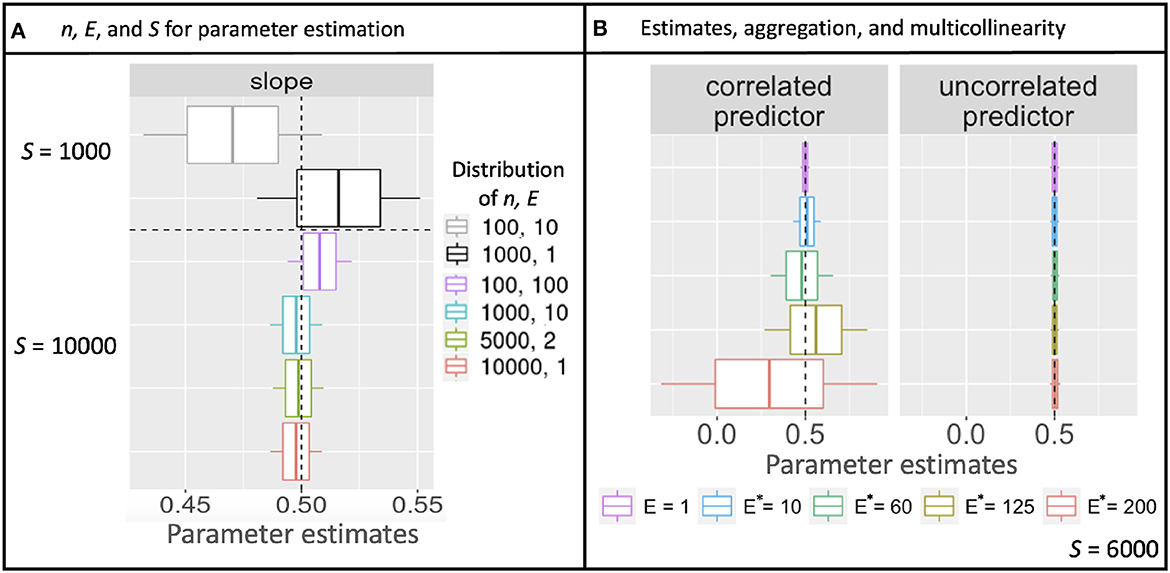
Figure 2. Uncertainty in slope estimates from simulated Poisson data. (A) Posterior mean parameter estimates diverge from the value used to simulate data (vertical dashed line) due to stochasticity, but parameter uncertainty (68% boxes and 95% whisker widths) are fixed for a given total sampling effort S, regardless of how it is partitioned by sample size n vs. observation effort E. (B) Where there is a correlated predictor (left panel), uncertainty in parameter estimates increases with aggregated effort E*, despite the same total effort S, but not for the uncorrelated predictor (right).
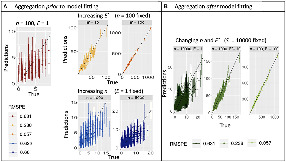
Figure 3. Out-of-sample true and predicted counts with corresponding root mean square prediction error for simulated data when aggregating before (A) and after (B) model fitting. (A) Increasing observation effort E improves predictions with reduced uncertainty, while increasing sample size n does not. The combination (n = 100, E = 1) plotted in dark red can be used as reference. (B) Predictions from a model fitted with E = 1 are dominated by noise, but can be rehabilitated by aggregation to E* = 10 or 1,000.
In the continuous case with within- and between-site variance (Equation 11), compositing measurements (increasing M) improves prediction when within-site (local) variance dominates (σ2 ≫ τ2). Conversely, when between-site variance dominates (τ2 ≫ σ2) compositing has little effect (Figure 4).
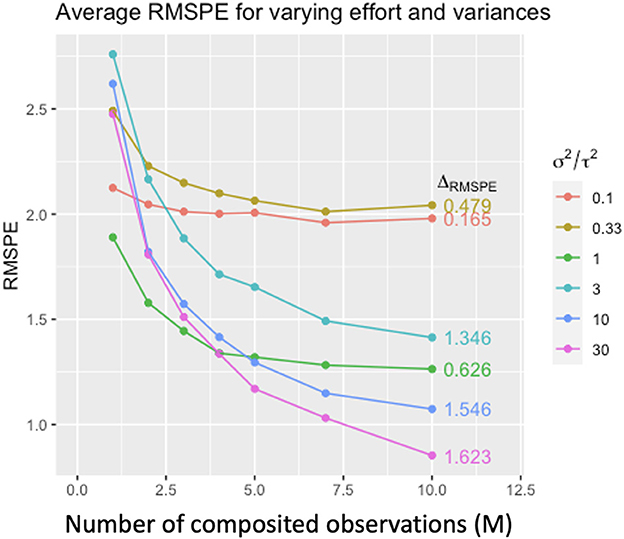
Figure 4. Average root mean square prediction error (RMSPE) for simulated composite Gaussian data under varying M (number of composited observations), within-site variance σ2 and between-site variance τ2. Colors denote the ratio σ2/τ2, and ΔRMSPE denotes the difference RMSPEM=1 − RMSPEM=10. Prediction performance improves with increasing M, but the amount of improvement depends on the relative magnitudes of σ2 and τ2. The more σ2 dominates τ2 (i.e., large σ2/τ2), the larger the improvement in predictive performance with increasing m (from ΔRMSPE = 0.165 in red to ΔRMSPE = 1.623, purple).
Simulations also examined parameter uncertainty in the scenario of correlated predictors. Parameter uncertainty increased with aggregation because predictor collinearity increased with the degree of aggregation E*, despite fixed sample effort S (Figure 2B). Unlike results with uncorrelated predictors, the parameter uncertainty with correlated predictors continues to increase with increasing aggregation.
The application to the FIA network described in Section 3.2 extends insights from analytics and simulation to a large network that responds to predictors on multiple scales. Our application is designed to explore how aggregation affects both parameter estimation and predictive performance in this complex network. We begin by discussing the affects on parameter estimation. Estimates for the effects of climate variables, soils, and stand age on basal area differ in their responses to the degree (J) and the method (covariate clustering vs. EPA ecoregions) of aggregation (Figure 5A). Uncertainty in parameter estimates decreases when moving from J = 1 to J = 10, but then increases slightly with increasing aggregation up to J = 200. This may be tied to a small increase in collinearity in predictors with large aggregated plot clusters (aggregated units of analysis) J (Figure 5B). The reduced uncertainty from J = 1 to J = 10 is unexpected due to the induced collinearity, but it comes with a large reduction in estimated residual variance (Figure 5C).
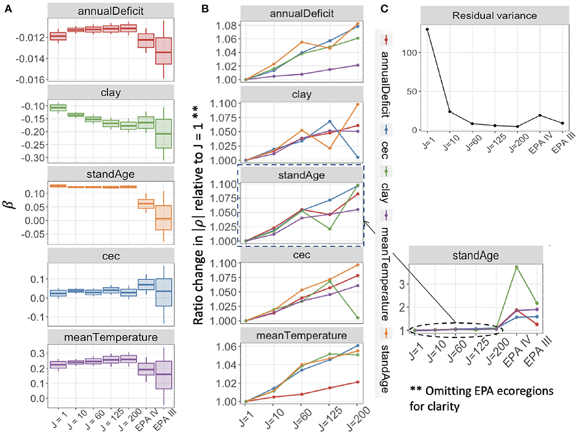
Figure 5. (A) Posterior mean estimates, with 68 and 95% credible intervals for coefficients in the Gaussian model for basal area with aggregation of FIA plots. Credible interval width shows modest increase with aggregation level from aggregations of J = 10 up to J = 200 plots, and large uncertainty at ecoregions (EPA III, IV). (B) Ratio change from J = 1 in magnitude of pairwise correlations between predictors in X increase slightly with aggregation by distance and covariate similarity (J = 1,…, 200) and then increase more dramatically at the ecoregion level (side panel). Colors in (B) denote the second variable that is pairwise correlated with each panel. (C) Estimated residual variance of each model decreases with J, with a large decrease from J = 1 to J = 10.
Ecoregion aggregation generates especially wide confidence intervals because ecoregions are not defined on the basis of covariates selected for their importance for trees (Supplementary Table 1B). Most coefficients from the EPA III aggregation have 95% credible intervals that include zero, and they diverge from estimates that come from aggregation based on covariate similarity, none of which have posterior 95% intervals that include zero (Figure 5A). Additionally, the collinearity in predictors at ecoregion aggregations is much larger than the collinearity for aggregations based on covariate similarity (Figure 5B).
The parameter estimates showing the largest increase in interval width with aggregation are those with regional-scale spatial correlation, including annual deficit, temperature, and clay. Stand age, which is not spatially correlated at scales that can be resolved at the FIA sampling density, does not show this increase in interval width with aggregation. However, the role of stand age is obliterated when aggregated to the ecoregion scale (Figure 5A).
For predictions on held-out data, prediction performance improves with aggregation by covariate similarity and distance up to at least J = 125, with the lowest RMSPE for J = 200. Prediction for level IV ecoregions is worse than for level III, despite level IV showing narrower confidence on parameter estimates (Figure 5A). If there is an optimal aggregation at which both parameter estimates are predictions are useful, it is in the range of 10 ≤ J ≤ 200.
Through analytical examples and an application to FIA data, we illustrate how data can be used to both understand ecological relationships and predict outcomes from statistical models is informed by the idea of few-large vs. many-small (FLvMS). Building up from analytical calculations, we establish a direct and quantifiable link between sample size and effort per observation (together, the total sampling effort) to uncertainty in parameter estimates and prediction. These relationships remain under simulation (Figures 2, 3), which, combined with a case study, extends results to spatially correlated predictors (Figure 5B). While the fact that correlation between covariates degrades information content has long been known (e.g., Dormann et al., 2013), our results place these relationships in the context of the FLvMS trade-off.
Our results demonstrate differing implications of FLvMS design for the goals of parameter estimation and prediction (Equations 9, 13). Parameter uncertainty depends on total sample effort S and not on how it is distributed across FLvMS (Figure 2A), though this relationship can be degraded by correlated predictors (Figure 2B). The extent to which this effort-dependence becomes important can change with the spatial scale of correlation, which can differ for each covariate (Figure 5B), or with changes in residual variance (Figure 5C). The application to FIA data illustrates that the underlying spatial patterns in the data (including omitted variables and spatial correlation between plots) might impact how much extra information is gained from larger plots vs. more plots [E vs. n; e.g., Nyyssönen and Vuokila (1963)]. For example, especially poor predictions for Level IV ecoregions in our application (Figure 6) are likely due to the incorporation of land use at Level IV that may not be relevant for forest biomass at this scale (Omernik and Griffith, 2014; Roman et al., 2018). Improved prediction with more plot aggregation in FIA reflects the dominant role of broad-scale climate for the distribution of forest abundance, just as prediction skill for precipitation can improve with an expanded spatial scale (Chardon et al., 2016). These results are especially focused on predicting basal area for trees in similar growing conditions, as is used for analyses within groupings like land use or habitat type (Carter et al., 2013; Thompson et al., 2017) but results may vary when predicting back out onto spatially contiguous groups of plots across habitat types. There are also likely unmeasured variables, conditions, or plots that skew results, which are especially important for accurate prediction at fine spatial scales.
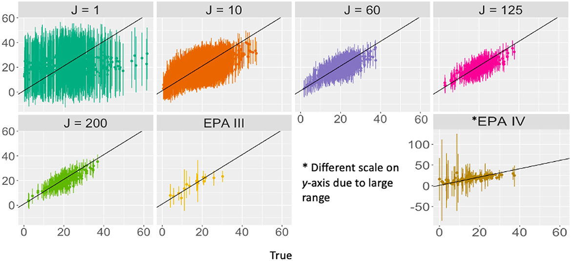
Figure 6. True and predicted total basal area with 95% prediction intervals at different levels of aggregation. Note that with the exception of EPA IV, the axes are the same across aggregations. Predicted TBA better approximates the truth for aggregated data (black y = x line provided for comparison), and prediction error decreases with aggregation.
The option to aggregate many small plots helps to achieve goals of both parameter estimation and prediction within the same network. Whereas a large plot averages away the role of fine-scale influences, small plots capture these local differences, while offering the option to aggregate. The hybrid design used by the National Ecological Observation Network (NEON) embeds many-small within regional sites, intended to capture multiple variables at multiple scales. If the many-small design seems optimal, it is important to appreciate how meaningful signal can degenerate into noise when effort is too low.
To be clear, we do not posit that one should always aggregate data during analysis. For example, if a sample consists of observations from each of a few very different ecoregions, aggregation would most likely lead to poorer inference. Additionally, not all data are suitable for aggregation. Two examples include: instances of the ecological fallacy - the assumption that what holds true for the group also holds true for an individual (Plantadosi et al., 1988), and relationships that shift based on the timescale examined [especially for seasonal responses, e.g., food webs (Jordán and Osváh, 2009)]. The authors also note that aggregation is most straightforward with data that can be averaged or summed into totals. As we demonstrate in our application to FIA data, the method of aggregation can greatly influence how much information can be extracted from the data.
Our results also point to the importance of knowing one's dataset and not relying on statistical tools alone to determine the relevance of environmental predictors. It can be tempting to use large datasets to search for the environmental covariates that produce the “best” predictions for a given response of interest. However, models that obtain the “best” predictions might not reveal meaningful ecological relationships. For example, using temperature and precipitation gradients is common practice to define species distribution models, and can be used successfully at global and regional scales (Elith and Leathwick, 2009). But those two metrics alone will not be as meaningful at the meter scale for many species, and modeling at that scale would have so much noise as to obscure the signal in the data. The conclusion, however, should not necessarily be that temperature and precipitation are irrelevant but perhaps that climatic impacts operate at larger scales than 1 m (Beaumont et al., 2005; Elith and Leathwick, 2009; Austin and Van Niel, 2010).
Focusing on the effects of FLvMS, post data collection, we intentionally omit fixed costs that can be associated with an observation, regardless of size [e.g., travel; Scott (1993); Henttonen and Kangas (2015)]. There are many factors that impact the cost of travel, including the road network, terrain, fuel costs, personnel costs, equipment portability, weather, and more [e.g., Morant et al. (2020); Lister and Leites (2022)] that would require economic modeling beyond the scope of this paper in order to be broadly applicable. Heavily-instrumented networks like NEON involving costly analytical techniques (e.g., soil and foliar biogeochemistry analytes) and heterogeneous responses (e.g., plant phenology as well as abundance and diversity) introduce additional considerations that are not included here.
The benefits and costs for parameter estimation and prediction from FLvMS designs take on new importance with large investments in sampling networks like FIA, NEON (Schimel, 2011), and the South African Ecological Observatory Network (SAEON; Van Jaarsveld et al., 2007). For example, from 2006 to 2016, the FIA program invested more than $20M annually to monitor tens of thousands of plots (Vogt and Smith, 2016, Table 3). Through 2024, annual operation costs for NEON are estimated to exceed $60M to make repeated observations of ecosystems that include vegetation plots of a similar size ((NSF, 2019), p. 16). These sampling networks can be invaluable for monitoring and also for understanding ecological processes and predicting future outcomes if the data are analyzed thoughtfully and the design facilitates these analysis goals. By extracting the contribution of FLvMS for parameter estimation and prediction, this analysis facilitates its consideration as one of many important components of data analysis and monitoring network design.
Publicly available datasets were analyzed in this study. This data can be found at: https://doi.org/10.7924/r43t9qf44.
BT, RK, and JC contributed to conception and design of the study. RK and JC organized the data. BT and JC designed and performed the statistical analysis. BT and RK wrote the first draft of the manuscript. JC and DB wrote sections of the manuscript. All authors contributed to manuscript revision, read, and approved the submitted version.
Funding came from National Science Foundation Graduate Research Fellowships (Program 1644868) to BT and RK, National Science Foundation Grant: DEB-1754443 and by the Belmont Forum (1854976), NASA (AIST16-0052 and AIST18-0063), and the Programme d'Investissement d'Avenir under project FORBIC (18-MPGA-0004; Make Our Planet Great Again) to JC. The National Ecological Observatory Network is a program sponsored by the National Science Foundation and operated under cooperative agreement by Battelle. This material is based in part upon work supported by the National Science Foundation through the NEON Program.
Tong Qiu helped develop code for clustering. Valentin Journ Rubn Palacio, Lane Scher, Shubhi Sharma, and Maggie Swift provided comments on the manuscript.
The authors declare that the research was conducted in the absence of any commercial or financial relationships that could be construed as a potential conflict of interest.
All claims expressed in this article are solely those of the authors and do not necessarily represent those of their affiliated organizations, or those of the publisher, the editors and the reviewers. Any product that may be evaluated in this article, or claim that may be made by its manufacturer, is not guaranteed or endorsed by the publisher.
The Supplementary Material for this article can be found online at: https://www.frontiersin.org/articles/10.3389/fevo.2023.1114569/full#supplementary-material
Abatzoglou, J. T., Dobrowski, S. Z., Parks, S. A., and Hegewisch, K. C. (2018). TerraClimate, a high-resolution global dataset of monthly climate and climatic water balance from 1958 to 2015. Sci. Data 2017, 191. doi: 10.1038/sdata.2017.191
Andelman, S. J., and Willig, M. R. (2004). Networks by design: A revolution in ecology. Science 305, 1565–1567. doi: 10.1126/science.305.5690.1565b
Anderson-Teixeira, K. J., Davies, S. J., Bennett, A. C., Gonzalez-Akre, E. B., Muller-Landau, H. C., Joseph Wright, S., et al. (2015). CTFS-ForestGEO: A worldwide network monitoring forests in an era of global change. Glob. Change Biol. 21, 528–549. doi: 10.1111/gcb.12712
Austin, M. P., and Van Niel, K. P. (2010). Improving species distribution models for climate change studies: Variable selection and scale. J. Biogeogr. 38, 1–8. doi: 10.1111/j.1365-2699.2010.02416.x
Barnett, D. T., and Stohlgren, T. J. (2003). A nested-intensity design for surveying plant diversity. Biodiv. Conserv. 12, 255–278. doi: 10.1023/A:1021939010065
Beaumont, L. J., Hughes, L., and Poulsen, M. (2005). Predicting species distributions: Use of climatic parameters in bioclim and its impact on predictions of species current and future distributions. Ecol. Model. 186, 251–270. doi: 10.1016/j.ecolmodel.2005.01.030
Brown, J. P., and Westfall, J. A. (2012). “An evaluation of the properties of the variance estimator used by FIA,” in 2010 Joint Meeting of the FIA Symposium and the Southern Mensurationists (Asheville, NC: U.S. Department of Agriculture Forest Service, Southern Research Station), 53–58.
Burrill, E. A., DiTommaso, A. M., Turner, J. A., Pugh, S. A., Menlove, J., Christiansen, G., et al. (2021). The Forest Inventory and Analysis Database: Database Description and User Guide Version 9.0.1 for Phase 2.
Carter, D. R., Fahey, R. T., and Bialecki, M. B. (2013). Tree growth and resilience to extreme drought across an urban land-use gradient. Arbocult. Urban Forest. 39, 279–285. doi: 10.48044/jauf.2013.036
Chardon, J., Favre, A.-C., and Hingray, B. (2016). Effects of spatial aggregation on the accuracy of statistically downscaled precipitation predictions. J. Hydrometeorol. 17, 1561–1578. doi: 10.1175/JHM-D-15-0031.1
Crewe, T. L., Taylor, P. D., and Lepage, D. (2016). Temporal aggregation of migration counts can improve accuracy and precision of trends. Avian Conserv. Ecol. 11, 208. doi: 10.5751/ACE-00907-110208
Dietze, M. C., Fox, A., Beck-Johnson, L. M., Betancourt, J. L., Hooten, M. B., Jarnevich, C. S., et al. (2018). Iterative near-term ecological forecasting: Needs, opportunities, and challenges. Proc. Natl. Acad. Sci. U. S. A. 115, 1424–1432. doi: 10.1073/pnas.1710231115
Dormann, C. F., Elith, J., Bacher, S., Buchmann, C., Carl, G., Carré, G., et al. (2013). Collinearity: A review of methods to deal with it and a simulation study evaluating their performance. Ecography 36, 27–46. doi: 10.1111/j.1600-0587.2012.07348.x
eBird (2017). eBird: An Online Database of Bird Distribution and Abundance [Web Application]. Ithaca; NY: Cornell Lab of Ornithology.
Elith, J., and Leathwick, J. R. (2009). Species distribution models: Ecological explanation and prediction across space and time. Ann. Rev. Ecol. Evol. Systemat. 40, 677–697. doi: 10.1146/annurev.ecolsys.110308.120159
Gray, A. N., Brandeis, T. J., Shaw, J. D., McWilliams, W. H., and Miles, P. D. (2012). Forest inventory and analysis database of the united states of america (fia). In Vegetation databases for the 21st century. Biodiversity and Ecology, eds. J. Dengler, J. Oldeland, F. Jansen, M. Chytry, J. Ewald, M. Finckh, F. Glockler, G. Lopez-Gonzalez, R. K. Peet, and J. H. J. Schaminee. Biodiv. Ecol. 4, 225–231. doi: 10.7809/b-e.vol_04
Gregoire, T. G., and Valentine, H. T. (2007). Sampling Strategies for Natural Resources and the Environment. Boca Raton, FL: CRC Press.
Hengl, T., Mendes de Jesus, J., Heuvelink, G. B. M., Ruiperez Gonzalez, M., Kilibarda, M., Blagotić, A., et al. (2017). SoilGrids250m: Global gridded soil information based on machine learning. PLoS ONE 12, 169748. doi: 10.1371/journal.pone.0169748
Henttonen, H. M., and Kangas, A. (2015). Optimal plot design in a multipurpose forest inventory. For. Ecosyst. 2, 1–14. doi: 10.1186/s40663-015-0055-2
Iverson, L. R., and Prasad, A. M. (1998). Predicting abundance of 80 tree species following climate change in the eastern united states. Ecol. Monogr. 68, 465–485. doi: 10.1890/0012-9615(1998)0680465:PAOTSF2.0.CO;2
Iwamura, T., Guzman-Holst, A., and Murray, K. A. (2020). Accelerating invasion potential of disease vector aedes aegypti under climate change. Nat. Commun. 11, 2130. doi: 10.1038/s41467-020-16010-4
Jelinski, D. E., and Wu, J. (1996). The modifiable areal unit problem and implications for landscape ecology. Landsc. Ecol. 11, 129–140. doi: 10.1007/BF02447512
Jordán, F., and Osváth, G. (2009). The sensitivity of food web topology to temporal data aggregation. Ecol. Model. 220, 3141–3146. doi: 10.1016/j.ecolmodel.2009.05.002
Liebhold, A., and Gurevitch, J. (2002). Integrating the statistical analysis of spatial data in ecology. Ecography 25, 553–557. doi: 10.1034/j.1600-0587.2002.250505.x
Lister, A. J., and Leites, L. P. (2022). Cost implications of cluster plot design choices for precise estimation of forest attributes in landscapes and forests of varying heterogeneity. Can. J. For. Res. 52, 188–200. doi: 10.1139/cjfr-2020-0509
Lo, A., Chernoff, H., Zheng, T., and Lo, S.-H. (2015). Why significant variables aren't automatically good predictors. Proc. Natl. Acad. Sci. U. S. A. 112, 13892–13897. doi: 10.1073/pnas.151828511
Maas-Hebner, K. G., Harte, M. J., Molina, N., Hughes, R. M., Schreck, C., and Yeakley, J. A. (2015). Combining and aggregating environmental data for status and trend assessments: challenges and approaches. Environ. Monitor. Assess. 187, 1–16. doi: 10.1007/s10661-015-4504-8
Malik, A., Rao, M. R., Puppala, N., Koouri, P., Thota, V. A. K., Liu, Q., et al. (2021). Data-driven wildfire risk prediction in Northern California. Atmosphere 12, 109. doi: 10.3390/atmos12010109
McRoberts, R. E., Chen, Q., Gormanson, D. D., and Walters, B. F. (2018). The shelf-life of airborne laser scanning data for enhancing forest inventory inferences. Remote Sens. Environ. 206, 254–259. doi: 10.1016/j.rse.2017.12.017
Morant, J., González-Oreja, J. A., Martínez, J. E., López-López, P., and Zuberogoitia, I. (2020). Applying economic and ecological criteria to design cost-effective monitoring for elusive species. Ecol. Indicat. 115, 106366. doi: 10.1016/j.ecolind.2020.106366
Neuendorf, K. A. (2021). “Unit of analysis and observation,” in Research Methods in the Social Sciences: an AZ of Key Concepts, eds J. F. Morin, C. Olsson, and E. O. Atikcan (New York, NY: Oxford University Press), 301–306.
NSF (2019). The National Ecological Observatory Network (NEON): FY 2019 NSF Budget Request to Congress. Washington, DC.
Nyyssönen, A., and Vuokila, Y. (1963). The effect of stratification on the number of sample plots of different sizes. Acta Forestalia Fennica. 75. doi: 10.14214/aff.7136
Omernik, J. M. (1987). Ecoregions of the conterminous united states. Ann. Assoc. Am. Geogr. 77, 118–125. doi: 10.1111/j.1467-8306.1987.tb00149.x
Omernik, J. N., and Griffith, G. E. (2014). Ecoregions of the conterminous united states: Evolution of a hierarchical spatial framework. Environ. Manag. 54, 1249–1266. doi: 10.1007/s00267-014-0364-1
Plantadosi, S., Byar, D. P., and Green, S. B. (1988). The ecological fallacy. Am. J. Epidemiol. 127, 893–904. doi: 10.1093/oxfordjournals.aje.a114892
Qiu, T., Sharma, S., Woodall, C., and Clark, J. (2021). Niche shifts from trees to fecundity to recruitment that determine species response to climate change. Front. Ecol. Evol. 9, 863. doi: 10.3389/fevo.2021.719141
R Core Team (2013). R: A Language and Environment for Statistical Computing. Vienna: R Foundation for Statistical Computing.
Roman, L. A., Pearsall, H., Eisenman, T. S., Conway, T. M., Fahey, R. T., Landry, S., et al. (2018). Human and biophysical legacies shape contemporary urban forests: A literature synthesis. Urban For. Urb. Green. 31, 157–168. doi: 10.1016/j.ufug.2018.03.004
Rossi, R. E., Mulla, D. J., Journel, A. G., and Franz, E. H. (1992). Geostatistical tools for modeling and interpreting ecological spatial dependence. Ecol. Monogr. 62, 277–314. doi: 10.2307/2937096
Schimel, D. (2011). The era of continental-scale ecology. Front. Ecol. Environ. 9, 311. doi: 10.1890/1540-9295-9.6.311
Schliep, E. M., Gelfand, A. E., Clark, J. S., and Zhu, K. (2016). Modeling change in forest biomass across the eastern us. Environ. Ecol. Stat. 23, 23–41. doi: 10.1007/s10651-015-0321-z
Scott, C. T. (1993). “Optimal design of a plot cluster for monitoring,” in Proceedings, IUFRO S.4.11 Conference (London: University of Greenwich), 233–242.
Singh, S., Nouri, A., Singh, S., Anapalli, S., Lee, J., Arelli, P., et al. (2020). Soil organic carbon and aggregation in response to 39 years of tillage management in the southeastern us. Soil Tillage Res. 197, 104523. doi: 10.1016/j.still.2019.104523
Tang, B., Clark, J. S., and Gelfand, A. E. (2021). Modeling spatially biased citizen science effort through the ebird database. Environ. Ecol. Stat. 28, 609–630. doi: 10.1007/s10651-021-00508-1
Thompson, D. K., Parisien, M.-A., Morin, J., Millard, K., Larsen, C. P., and Simpson, B. (2017). Fuel accumulation in a high-frequency boreal wildfire regime: From wetland to upland. Can. J. For. Res. 47, 957–964. doi: 10.1139/cjfr-2016-0475
Tinkham, W. T., Mahoney, P. R., Hudak, A. T., Domke, G. M., Falkowski, M. J., Woodall, C. W., et al. (2018). Applications of the united states forest inventory and analysis dataset: A review and future directions. Can. J. For. Res. 48, 1251–1268. doi: 10.1139/cjfr-2018-0196
Van Jaarsveld, A. S., Pauw, J. C., Mundree, S., Mecenero, S., Coetzee, B. W., and Alard, G. F. (2007). South african environmental observation network: Vision, design and status: SAEON reviews. South Afr. J. Sci. 103, 289–294.
Vogt, J. T., and Smith, W. B. (2016). Forest Inventory and Analysis Fiscal Year 2015 Business Report. Government Printing Office.
Wang, G., Gertner, G., Howard, H., and Anderson, A. (2008). Optimal spatial resolution for collection of ground data and multi-sensor image mapping of a soil erosion cover factor. J. Environ. Manag. 88, 1088–1098. doi: 10.1016/j.jenvman.2007.05.014
Wang, G., Gertner, G., Xiao, X., Wente, S., and Anderson, A. B. (2001). Appropriate plot size and spatial resolution for mapping multiple vegetation types. Photogrammetr. Eng. Remote Sens. 67, 575–584.
Wintle, B. A., Runge, M. C., and Bekessy, S. A. (2010). Allocating monitoring effort in the face of unknown unknowns. Ecol. Lett. 13, 1325–1337. doi: 10.1111/j.1461-0248.2010.01514.x
Yim, J.-S., Shin, M.-Y., Son, Y., and Kleinn, C. (2015). Cluster plot optimization for a large area forest resource inventory in Korea. For. Sci. Technol. 11, 139–146. doi: 10.1080/21580103.2014.968222
Zeide, B. (1980). Plot size optimization. For. Sci. 26, 251–257. doi: 10.1093/forestscience/26.2.251
Keywords: aggregation, clustering, Forest Inventory and Analysis (FIA), parameter uncertainty, prediction performance, sample design, sampling effort
Citation: Tang B, Kamakura RP, Barnett DT and Clark JS (2023) Learning from monitoring networks: Few-large vs. many-small plots and multi-scale analysis. Front. Ecol. Evol. 11:1114569. doi: 10.3389/fevo.2023.1114569
Received: 02 December 2022; Accepted: 20 March 2023;
Published: 04 April 2023.
Edited by:
Pave Alain, Claude Bernard University, FranceReviewed by:
Zhiming Zhang, Yunnan University, ChinaCopyright © 2023 Tang, Kamakura, Barnett and Clark. This is an open-access article distributed under the terms of the Creative Commons Attribution License (CC BY). The use, distribution or reproduction in other forums is permitted, provided the original author(s) and the copyright owner(s) are credited and that the original publication in this journal is cited, in accordance with accepted academic practice. No use, distribution or reproduction is permitted which does not comply with these terms.
*Correspondence: Becky Tang, YnRhbmdAbWlkZGxlYnVyeS5lZHU=
†These authors have contributed equally to this work
Disclaimer: All claims expressed in this article are solely those of the authors and do not necessarily represent those of their affiliated organizations, or those of the publisher, the editors and the reviewers. Any product that may be evaluated in this article or claim that may be made by its manufacturer is not guaranteed or endorsed by the publisher.
Research integrity at Frontiers
Learn more about the work of our research integrity team to safeguard the quality of each article we publish.