
95% of researchers rate our articles as excellent or good
Learn more about the work of our research integrity team to safeguard the quality of each article we publish.
Find out more
ORIGINAL RESEARCH article
Front. Ecol. Evol. , 03 March 2023
Sec. Models in Ecology and Evolution
Volume 11 - 2023 | https://doi.org/10.3389/fevo.2023.1108739
Species richness and evenness have been widely used to investigate the spatiotemporal variation of α-diversity. However, some studies have indicated that a negative relationship exists between species richness and evenness. The question is how the differing sensitivity of α-diversity metrics and interactive behavior between richness and evenness affect the modeling of α-diversity variation. Here, we explored the response of species diversity, represented by three Hill numbers (i.e., species richness, exponential of Shannon index – expShannon, and inverse of Simpson index – invSimpson) focusing on the abundance of rare and common species, and Pielou index underlining the evenness of a community, to α-diversity variation through structural equation modeling (SEM). The model scheme integrated three categories of variables, spectral variation hypothesis (SVH), community pattern, and vertical structure, along the precipitation gradient spanning three steppes, including meadow steppe, typical steppe, and desert steppe. Our results showed that there were large differences in species richness across the three steppes, with v-shaped patterns emerging along the gradient (low-point in the typical steppe). Differences between steppes were diminished in the expShannon or invSimpson indices, though the v-shaped patterns persisted. The Pielou index showed the opposite pattern, with the peak in the typical steppe. Accordingly, a negative relationship between species richness and Pielou index was found across the three steppes. The concurrent increases in annual species number and dominant species abundance in response to precipitation variations led to the negative relationship. As a result, the SEM fitness on expShannon and invSimpson indices over the region was substantially diminished by the negative relationship. Overall, community pattern better explained the variation in species richness, invSimpson and Pielou indices. The performance of SVH differed among α-diversity metrics due to the collinearity with the variables of community pattern and vertical structure. This study emphasizes the variability of α-diversity metrics in response to environmental change. Particularly, distinguishing the asynchronous behaviors between species richness and evenness is paramount to account for α-diversity variation over heterogeneous ecosystems.
Grasslands are among the most species-rich habitats on Earth, possessing a high proportion of the world’s plant and animal life forms, but nowadays they are confronted with unprecedented challenges due to climate change and anthropogenic activity (Cleland et al., 2013; Fauvel et al., 2020). Globally, 37% of grasslands are fragmented, and temperate grasslands have lost about 46% of their area due to widespread agricultural expansion and intensive grazing regiments (Petermann and Buzhdygan, 2021). Accounting for various precipitation and temperature regimes, differing grassland species comprise the majority of Eurasian temperate grasslands, which results in complicated community structures and species composition (Sugita et al., 2007). Grassland species are relatively small in size compared to organisms from other biomes, but they greatly enrich a community in their large numbers. The species height of a community in the temperate steppes (e.g., desert, typical and meadow steppes) is ranged between about 4 cm and 30 cm, and determined by climate-relevant dominant species (e.g., Stipa breviflora, Leymus chinensis, and Stipa baicalensis; Bai et al., 2008; Xu et al., 2020). In the face of climate change and intensive land use, increasing studies demonstrate that native species are being lost from communities while toxic weeds grow in prevalence (Liu et al., 2013). This is expected to manifest in unpredictable changes in ecosystem services (e.g., livestock production), as well as impacts on carbon and nutrient cycles (Qiu and Cardinale, 2020). The lack of knowledge regarding how the asynchronous response of species relates to heterogeneous habitats and environmental change hinders an in-depth understanding of grassland biodiversity variation (Ryabov et al., 2022).
In general, variation in grassland species diversity can be explained by the theory of species coexistence (Questad and Foster, 2008). Essential mechanisms for species coexistence are competition and niche heterogeneity consociated with the local environmental conditions (Chesson, 2000). Numerous studies have shown that increased precipitation facilitates the survival of ruderal species and allows rare species to coexist with dominant species (Currie et al., 2004; Cleland et al., 2013; Figure 1). Consequently, evenness in species tends to decline in these circumstances due to the shifting abundance of the dominant species (Kardol et al., 2010). The adverse variations between species richness and evenness yield an asynchronous response of species diversity (DeJong, 1975; Stirling and Wilsey, 2001; Zhang et al., 2012). Trampling by herbivores and the excreta they produce can create more available niches, promoting synchronous increases in species richness and evenness (Golodets et al., 2011). However, selective feeding by large herbivores can lead to a homogeneous community structure and composition (Zhu et al., 2012). These asynchronous and/or synchronous influences associated with fluctuating precipitation and grazing practices reveal unpredictable variations in species diversity (Hauser et al., 2021).
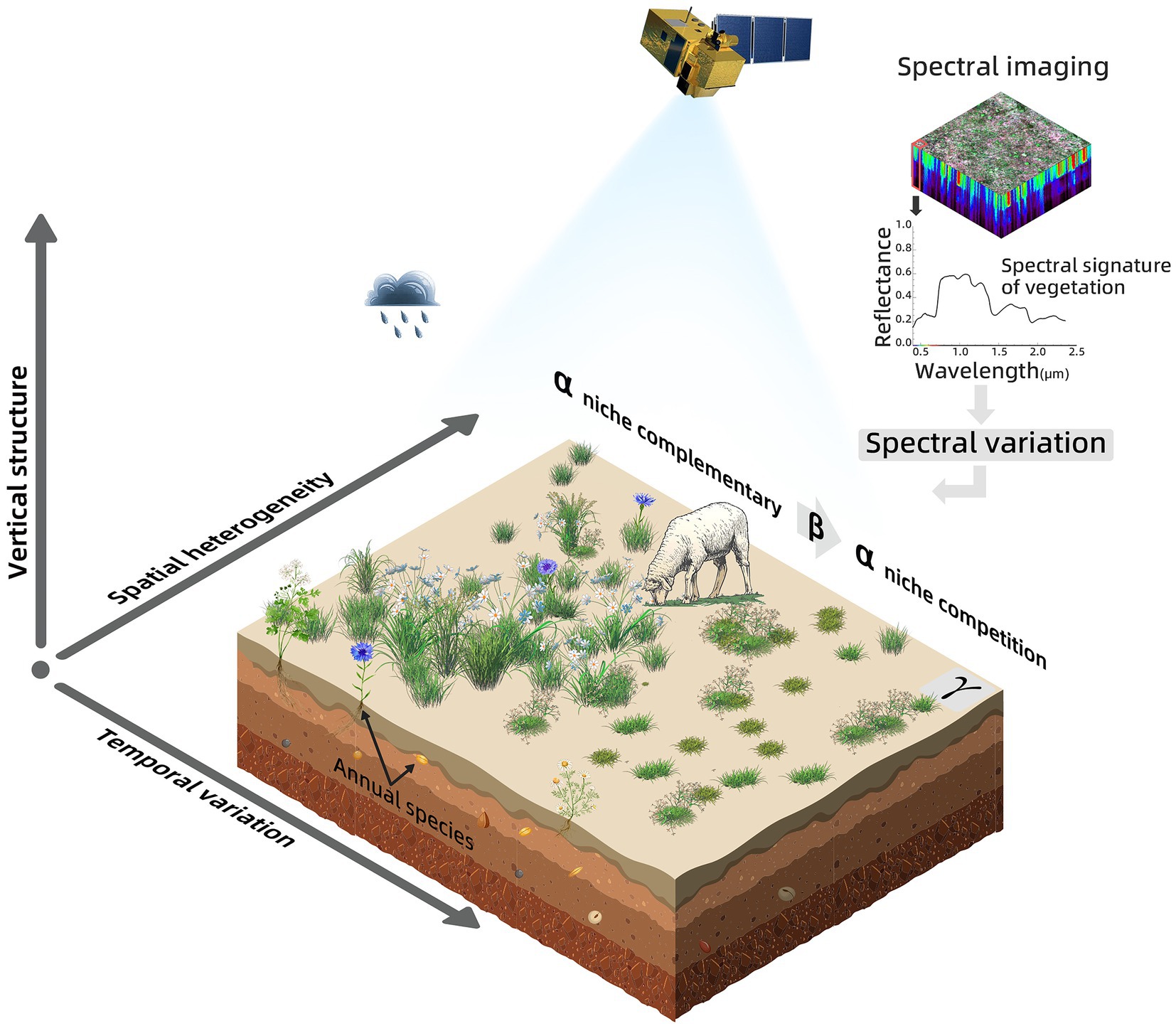
Figure 1. Theoretical framework depicting grassland species diversity through horizontal community pattern, vertical structure variables, and SVH. Precipitation and grazing practices lead to variation in species diversity across α-, β- and γ-scales, while the SVH is expected to detect diversity variation in the horizontal and vertical categories. The horizontal community pattern shows the competitive relationship among species in a community, termed a mixed pixel in SVH. The vertical structure shows the grass height heterogeneity, which reflects the response of diversity to precipitation and grazing practice.
Species diversity is scale-dependent and can be partitioned into α-, β- and γ-diversity, corresponding to the local, regional, and global scale, respectively (Whittaker, 1960). In general, under an equal level of γ-diversity, the communities with high α-diversity are more stable than those with low α-diversity (Wang et al., 2021; Figure 1). To date, the spectral variation hypothesis (SVH), which is supposed to connect the habitat heterogeneity and the composition of a community with spectral properties (Palmer et al., 2002), has been widely used to map α-diversity. However, the ability to identify taxonomic species using spectral properties can be diminished when the granularity of resolution exceeds approximately 10 cm (Wang et al., 2018). With coarse multispectral image data (e.g., above 0.5 m; Wang et al., 2022), the ability of SVH to account for the small-sized individuals of grass species is considerably restricted because multiple species are included in a pixel cell. Furthermore, due to the complex vertical layered properties of the community, the electromagnetic spectrum is incapable of penetrating the intensive overlap to detect the grass individual successfully. This is an additional error source to be aware of when using SVH (Thornley et al., 2022).
Empirical studies have shown that species diversity is closely associated with vertical structure, horizontal community pattern, and physiological properties (Loreau, 2000; Marselis et al., 2020). Vertical structure describes the height heterogeneity among species in a community, and horizontal community pattern reflects the intricate interaction between species at a population level (McCann et al., 2005). These two physical properties have been widely used to explore species diversity (Navarrete and Berlow, 2006; Gholizadeh et al., 2022). Using SVH partially expresses the variation of a biophysical relationship, but it is limited in detecting the details of horizontal and vertical features, and so constrains the accuracy to under 50% (Schmidtlein and Fassnacht, 2017; Thornley et al., 2022). In the face of the various steppe types (e.g., desert, typical, and meadow steppe), the effectiveness of SVH to reflect independent variations in α-diversity metrics and their interactions have not been fully explored. Ideally, integrating spectral variation with physical measures of both vertical and horizontal categories facilitates species diversity detection in grasslands (Wang and Gamon, 2019). For example, by combining vegetation structure data with airborne spectral images, species diversity can be calculated more accurately across the different growth stages of the grasses (Marcinkowska-Ochtyra et al., 2018) or in the degraded grassland disturbed by shrub encroachment (Sankey et al., 2021). Here, we questioned how effective this integration applies in identifying variations in species diversity across differing temperate steppes. Physical measures from the vertical structure and horizontal traits are inferred to improve the ability of SVH.
To accomplish this, we integrated the three categories of vertical structure, horizontal community pattern, and SVH to characterize variation in α-diversity and to systematically investigate how α-diversity metrics respond to variation in α-diversity over differing grassland types. We hypothesized that α-diversity could be comprehensively displayed by vertical structure, community pattern, and SVH associated with physiological properties (Marselis et al., 2020). In this case, the sensitivity of SVH variables to α-diversity could be co-influenced by the variation in vertical structure and community pattern due to the compounding response of the electromagnetic spectrum to community complexity (Thornley et al., 2022). Among widely used α-diversity metrics, three Hill numbers (i.e., species richness, exponential of Shannon index, and inverse of Simpson index) and the Pielou index were selected for both assessing abundance- and evenness-based species diversity (Pielou, 1966; Hill, 1973). Accordingly, we outline three objectives of interest, including (i) the independent and interactive behavior of α-diversity metrics in responding to precipitation variation; (ii) the performance of individual categories of explanatory variables in interpreting the variation in α-diversity metrics; (iii) the integrated performance of those three categories in depicting α-diversity variation, focusing on the boundedness of using SVH.
This study was conducted in the Eurasia steppe region of the Inner Mongolia Autonomous Region (IMAR) of northern China (Figure 2), which has a semi-arid and arid continental climate in the middle temperate zone. The study sites encompass three grassland types from east to west; meadow steppe (MS; 48.66°N, 119.13°E), typical steppe (TS; 44.14°N, 116.51°E), and desert steppe (DS; 41.77°N, 110.57–61°E). Over 1,125 km wide, the elevation ranges from 600 m in the east to 1,300 m in the west. Based on long-term meteorological observations (1980–2017), the mean annual temperature (MAT) ranged from −2.9°C to 6.5°C, with averages of −0.9°C, 3.1°C, and 4.8°C for MS, TS, and DS, respectively. The mean annual precipitation (MAP) ranged from 142.2 mm to 590.8 mm, with averages of 332.5 mm, 309.2 mm, and 279 mm for MS, TS, and DS, respectively. Most precipitation occurs from May to August. The soil is classified as chestnut and calcic brown (Bai et al., 2008). The MS is dominated by species Leymus chinensis, Carex duriuscula, and Stipa baicalensis. The TS is dominated by Stipa krylovii, Cleistogenes squarrosa, and Leymus chinensis. The DS is dominated by Stipa breviflora, Agropyron desertorum, and Cleistogenes songorica.
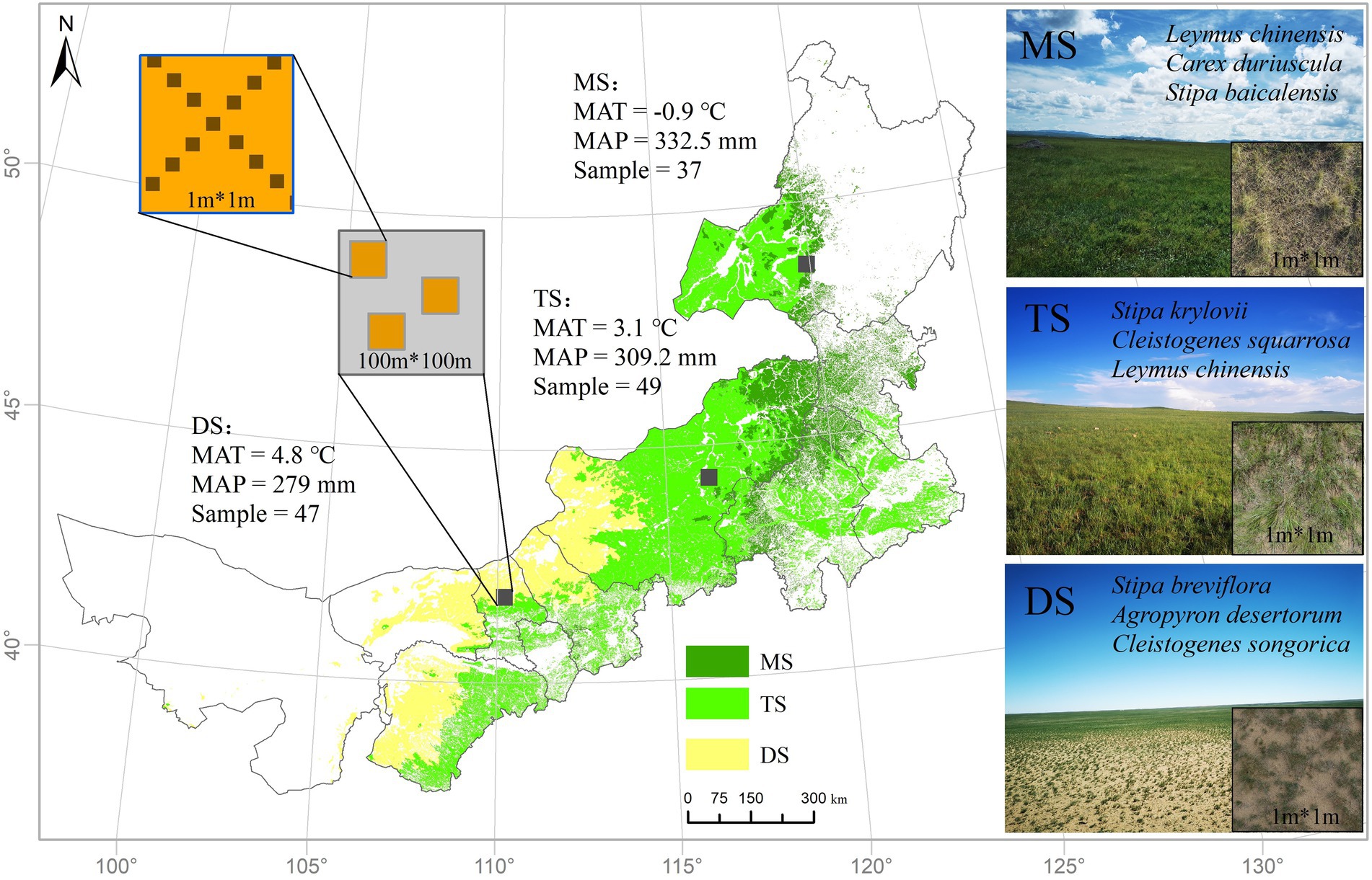
Figure 2. Overview of the study sites: meadow steppe (MS), typical steppe (TS), desert steppe (DS). Three landscape images are correspondingly presented on the right panel. Three 100 m*100 m plots were set up in each steppe type. Quadrats (1 m*1 m) in the north–south direction were located along two diagonal lines within each plot at an interval of approximately 14 m.
This study utilized multispectral satellite image data, species ground-truth survey data, and vertically projected RGB images of the quadrats. The multispectral satellite image data was obtained from the Sentinel-2A satellite, which was launched by the European Space Agency in 2015. Every 10 days, the satellite revisits the same viewing angles. A multispectral instrument (MSI) with 13 bands is mounted on the sentinel-2A satellite. Four bands are at 10 m spatial resolution, and six bands are at 20 m spatial resolution. In addition, there are three bands for atmospheric correction and cirrus cloud detection at 60 m spatial resolution. The reflectance bands at the finest resolution of 10 m were used in the study; blue (492.4 nm), green (559.8 nm), red (664.6 nm), and near-infrared (832.8 nm). Sentinel-2A Level 2A images were orthographic-corrected reflectance products at the bottom layer of the atmosphere and acquired from the European Space Agency Copernicus Open Access Hub.1 The collected images were free of clouds and cirrus contamination over the study sites. The acquired multispectral images were dated 7 July for DS, 21 June for TS, and 11 July for MS, which aligns with the timing of the fieldwork in 2020. We extracted the pixel reflectance values from the four bands using the central coordination of quadrats in the R-package “raster” (Hijmans, 2022; R Core Team, 2022).
Grassland species were investigated during fieldwork in the mid-growing season in June and July 2020. Three 100 m*100 m plots were set up in each steppe type, oriented in a north–south direction, and quadrats (1 m*1 m) were demarcated along two diagonal lines within each plot at intervals of approximately 14 m (Figure 2). This interval of 14 m was selected to ensure that each quadrat aligns to one 10 m-pixel from the multispectral image. In total, there were 37 quadrats in MS, 49 quadrats in TS, and 47 quadrats in DS. Each quadrat was situated around a central point identified by Real Time Kinematic- Global Navigation Satellite System (RTK-GNSS) to form a north–south oriented square with an accuracy of 0.01 m. After the demarcation, we recorded the name and individual count of each species falling into each quadrat. The height of individual species was measured in succession three times. The aboveground biomass of each species was weighed after harvesting and drying.
α-diversity was measured by the Hill number and Pielou index (Table 1). The Hill number, considered the ideal for quantifying abundance-based species diversity (Chao et al., 2014), is delineated by a single formula and the scaling value of exponent “q” which thus result in species richness (q = 0), exponential of Shannon index (expShannon index; q = 1) and inverse of Simpson index (invSimpson index; q = 2; Hill, 1973). Species richness includes all species regardless of their abundance and therefore weights rare and dominant species equally. ExpShannon and invSimpson indices both account for the abundance of all species. InvSimpson index reports the dominant species in a quadrat. ExpShannon index is an indicator of common species in a quadrat, retaining the sensitivity of species richness and the robustness of the invSimpson index (Roswell et al., 2021). The Pielou index describes the evenness of a quadrat (Pielou, 1966). These diversity metrics were computed using R-package “vegan” (Oksanen et al., 2022; R Core Team, 2022).
Spectral angle and vegetation index were used as a proxy for SVH. Taking the reflectance of four spectral bands (i.e., blue, green, red, and near-infrared), we calculated the six spectral angles between each of the two bands (i.e., SAbg, SAbr, SAbN, SAgr, SAgN, and SArN). In addition, we computed normalized difference vegetation index (NDVI) and enhanced vegetation index (EVI) based on the red, NIR, and blue bands (Table 2). Eventually, six spectral angles and two vegetation indices were used to reflect the SVH properties. Vertical structure variation was depicted by interspecies height variation. The average (Hmean), standard deviation (Hstd), and coefficient variation (Hcv) of interspecific height were calculated for each quadrat during fieldwork.
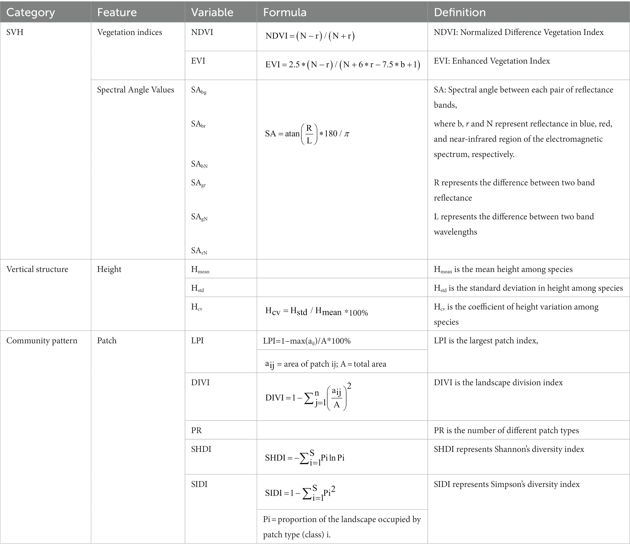
Table 2. Summary of the variables in the three-categories: SVH, vertical structure, and community pattern.
To access the community pattern of each quadrat, we captured true-color photos vertically with the camera. Each true-color photo was digitally interpreted by experts according to the color, texture, and shape in the ArcGIS 10.6 software (ESRI, 2017 Redlands, California, United States). Then interpreted photos were transformed into.fbt file format, and FRAGSTATS 4.2 (McGarigal and Marks, 1995) was used to obtain community pattern variables. Five variables were used to depict the community pattern, including the largest patch index (LPI), landscape division index (DIVI), patch richness (PR), landscape Shannon’s diversity index (SHDI), and landscape Simpson’s diversity index (SIDI) (Table 2). LPI is the percentage of the largest heterogeneous patch area comprised within the plot. As the largest patch area increases, LPI approaches 100%. DIVI represents the probability of two randomly chosen pixels in the quadrat belonging to the same patch type. PR is the number of different patch types presented in the quadrat.
We used multivariate analysis of variance (ANOVA) to examine whether α-diversity differed significantly between steppe types along a precipitation gradient. ANOVA analyses were repeatedly implemented over the region and the individual steppes. The dependent variables were the three Hill numbers (i.e., species richness, expShannon, and invSimpson indices) and the Pielou index, and the fixed factor was the steppe type. The results of ANOVA with p < 0.05 were considered statistically significant. Duncan’s multiple comparisons were used as a post hoc analysis to test for significant differences among all steppe types.
Pearson correlation with a two-tailed significance test was used to explore the relationship between the α-diversity index and each explanatory variable. Relationships were statistically significant at p < 0.05. A simple linear model with two-variable regression was used to examine the relationship of the three categorized variables against each diversity index across the three steppes. Pearson correlations were conducted for each explanatory variable across the three steppes as part of the variable selection process. To cross-compare the strength of the three categories of variables in characterizing α-diversity metrics, all data were normalized by subtracting the average and then dividing by the standard deviation prior to the regression modeling. An F-test was used to see if the linear regression was significant (p < 0.05). A higher regression coefficient of explanatory variables indicated a more competitive candidate for depicting variation in α-diversity.
Structural equation modeling (SEM) can be used to explore the direct and indirect influences among multiple variables as well as their integrated contribution to the independent variable (Rosseel, 2012). By constructing the SEM, we can examine the significant connections between exploratory variables and the α-diversity index as well as analyze the dependent relationship between exploratory variables through the standardized path coefficient (rp). As illustrated by Figure 3, there are three major pathways that reflect the direct effects of SVH on α-diversity and another two pathways that reflect the dependent effects of vertical structure and community pattern on spectral variables. The quality of the SEM was evaluated by comparative fit index (CFI) > 0.9, root mean square error of approximation (RMSEA) < 0.05, and standardized root mean square residual (SRMR) < 0.05 (Hooper et al., 2008). The significance level of modeling is graded by p < 0.05. The “lavaan” package in R was used to establish the SEM based on maximum likelihood estimation (Rosseel, 2012). All data used in the SEM were normalized by subtracting the average and then dividing by the standard deviation before modeling to compare the rp between the three categorized variables. Given the availability of sample data for the study, the modeling of species diversity using SEM was implemented for the entire region, aggregating the three steppes together.
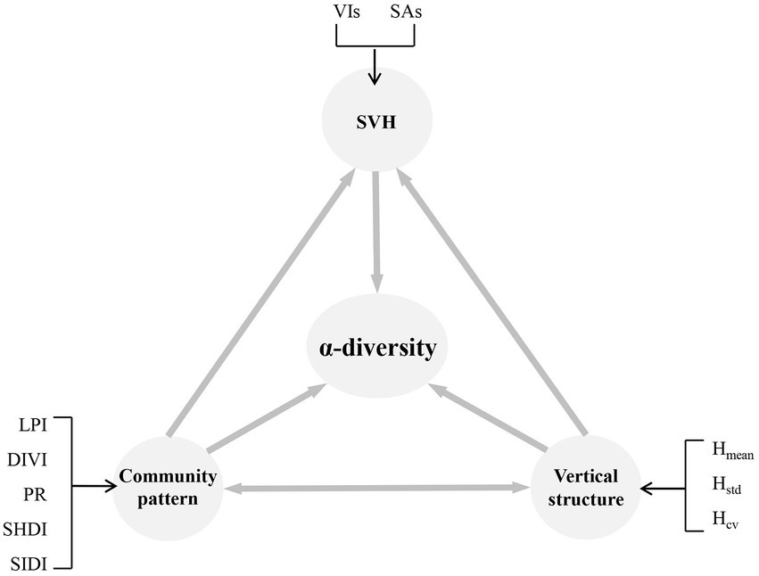
Figure 3. Model framework illustrating causal relationships between vertical structure, community pattern, SVH, and α-diversity. The impact of SVH on α-diversity is co-influenced by community pattern and vertical structure. SVH is described by vegetation indices (VIs) and spectral angle values (SAs), while community pattern is described by the largest patch index (LPI), landscape division index (DIVI), patch richness (PR), landscape Shannon’s diversity index (SHDI) and landscape Simpson’s diversity index (SIDI). The vertical structure was represented by interspecies height heterogeneity, including the average (Hmean), standard deviation (Hstd), and coefficient variation (Hcv).
Significant differences were observed in the four metrics of α-diversity along the precipitation gradient, which ranged from 332.5 mm for MS to 309.2 mm for TS to 279 mm for DS (p < 0.05; Figure 4). V-shaped patterns were observed in the three Hill numbers (i.e., species richness, expShannon, and invSimpson indices). There were large differences in species richness between steppes, and the TS was the least diverse (Figure 4A). When expShannon index was used, there was an insignificant difference between MS and DS (p > 0.05; Figure 4B), but when invSimpson index was used, the difference between MS and TS was insignificant (p > 0.05; Figure 4C). With the three Hill numbers, which evaluated rarity to a lesser degree than the Pielou index, MS, which had many rare species, became less diverse compared to TS and DS. DS had higher species richness in the expShannon and invSimpson indices than TS. The Pielou index showed the opposite pattern with the peak in TS (Figure 4D). Overall, the α-diversity metrics followed divergent patterns of variation over the region.
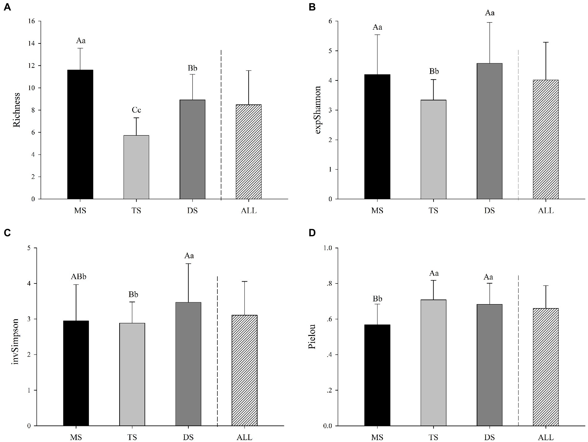
Figure 4. α-diversity metrics distribution and the one-way ANOVA result for three steppes. Upper case and lower case letters indicate significance at p < 0.01 and p < 0.05, respectively. ALL is an aggregate metric including all three steppe types; (A) species richness, (B) expShannon index, (C) invSimpson index, and (D) Pielou index. The error bars indicate the standard deviation (std).
A negative relationship was observed between species richness and Pielou index (r = −0.37, p < 0.001; Figure 5A) over the three steppes. In particular, there was a strong negative relationship between species richness and the Pielou index in TS (r = −0.54, p < 0.001; Figure 5C). In contrast, species richness and the Pielou index had insignificant relationships in MS (r = 0.09, p = 0.585; Figure 5B) and DS (r = 0.09, p = 0.526; Figure 5D). The aggregate data representing the full region showed that the expShannon index correlated most to species richness (r = 0.56, p < 0.05; Figure 5A), and the invSimpson index correlated most to the Pielou index (r = 0.68, p < 0.05; Figure 5A). Specifically, the expShannon and invSimpson indices correlated to the Pielou index more strongly than to species richness in MS (r = 0.94 and 0.94, p < 0.05; Figure 5B) and DS (r = 0.76 and 0.85, p < 0.05; Figure 5D). In contrast, the expShannon index correlated to species richness more than to the Pielou index in TS (r = 0.61, p < 0.05; Figure 5C). This implies that the relationship of α-diversity indices at a local scale could strongly influence the overall relationship across the region.
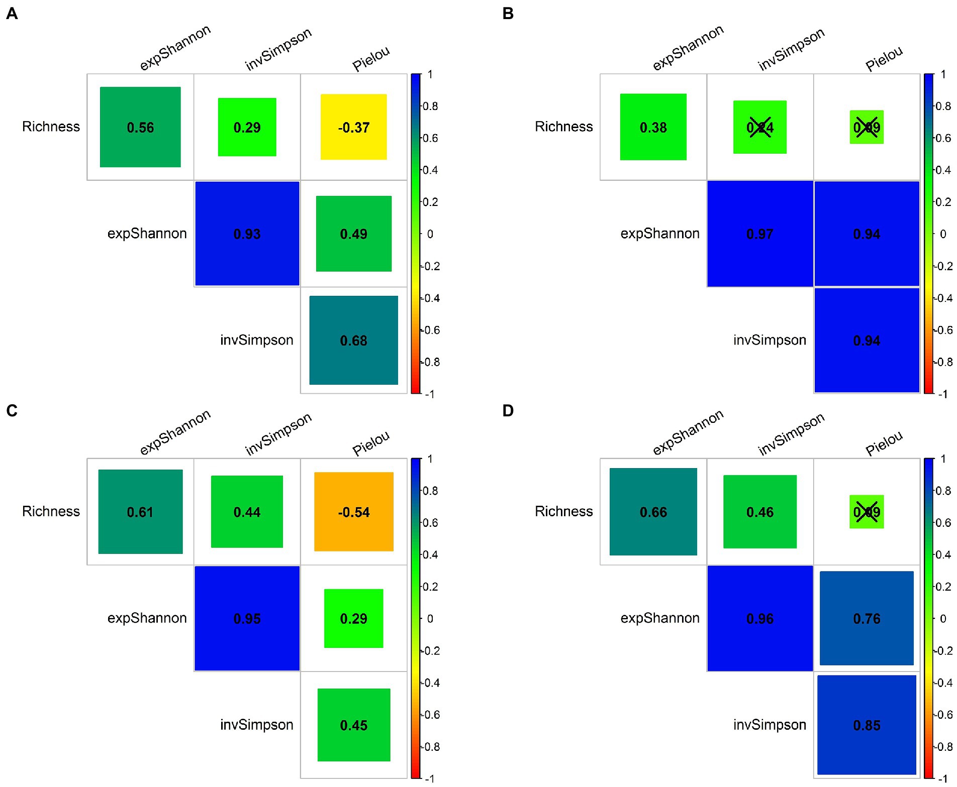
Figure 5. Correlation heat map of the species diversity metrics across the study sites. Pearson’s correlation coefficients are shown in each square. The yellow-red color indicates a negative correlation, and the green-blue color indicates a positive correlation. Correlation coefficients with p > 0.05 are marked with a cross. (A) The aggregate of three grassland types, (B) MS, (C) TS, and (D) DS.
Correlations between α-diversity indices and the many variables varied in their strength, with r ranging from 0.01 to 0.69 (Figure 6). Hmean, Hstd, SArN, and PR significantly explained the variation in species richness, with r-values of −0.69, −0.63, −0.64, and 0.61, respectively. Hmean, Hstd, PR, NDVI, and EVI significantly correlated to the expShannon index, with r-values of −0.45, −0.45, 0.49, −0.46, and − 0.46, respectively. Hmean, Hstd, PR, and EVI significantly explained variation in the invSimpson index, with r-values of −0.24, −0.26, 0.35, and − 0.30, respectively. The Pielou index was significantly explained by Hmean, DIVI, LPI, and SIDI, with r-values of 0.32, 0.44, −0.41, and 0.41, respectively. Vertical structure and SVH variables explained species richness variation among α-diversity metrics well, while community pattern variables characterized the Pielou index better.
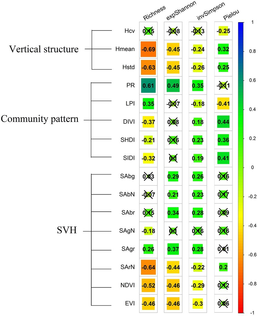
Figure 6. Pearson correlations between SVH, community pattern, vertical structure variables, and α-diversity metrics across three steppes. Pearson correlation coefficients are shown in each square. The yellow-red color indicates a negative correlation, and the green-blue color indicates a positive correlation. Correlation coefficients at a significance level of p > 0.05 were marked with a cross.
Responses of vertical structure and community pattern variables to species richness and the Pielou index were asynchronous. Hmean and Hstd correlated strongly and negatively to species richness (r = −0.69 and − 0.63, p < 0.001), but they correlated slightly positively to the Pielou index (r = 0.32 and 0.25, p < 0.01). Meanwhile, PR and LPI correlated moderately and positively to species richness (r = 0.61 and 0.35, p < 0.001), but they correlated negatively to the Pielou index, with r-values of −0.11 and − 0.41, respectively. The scenario also appeared in SVH variables. Overall, SArN, NDVI, and EVI correlated strongly and negatively to species richness (−0.64 < r < −0.46, p < 0.001) but weakly and positively to the Pielou index (0.06 < r < 0.20, 0.02 < p < 0.50).
The slopes of the two-variable regressions also indicated the asymmetrical responses of explanatory variables (i.e., vertical structure, community pattern, and SVH) to variation in α-diversity (Figure 7). The fitted surfaces of species richness were negatively related to those of the Pielou index (Figures 7A,D). In contrast, slopes of the fitted surfaces of the expShannon and invSimpson indices are gentle compared to the sharp and opposite slopes for species richness and evenness (Figures 7B,C). Variation in species richness (0.44 < R2 < 0.51; Figure 7A) and the expShannon index (0.20 < R2 < 0.24; Figure 7B) were better explained than the invSimpson (0.05 < R2 < 0.15; Figure 7C) and Pielou indices (0.088 < R2 < 0.14; Figure 7D). Hmean negatively related to species richness (slope = −0.69, p < 0.001) and positively affected the Pielou index (slope = 0.53, p < 0.01). Hstd was more influential on the Pielou index (slope = −0.23, p = 0.25). Hmean and Hstd were important and complementary in describing α-diversity. For the community pattern variables, SHDI was better at describing the Pielou index (slope = 0.38, p < 0.001). In addition, NDVI outperformed other SVH variables in characterizing the variation in Pielou index (slope = 0.76, p < 0.001) and Hill numbers, with the slope of −1.59, −0.71, and − 0.18 for species richness (p < 0.001), expShannon index (p < 0.001) and invSimpson index (p = 0.37), respectively.
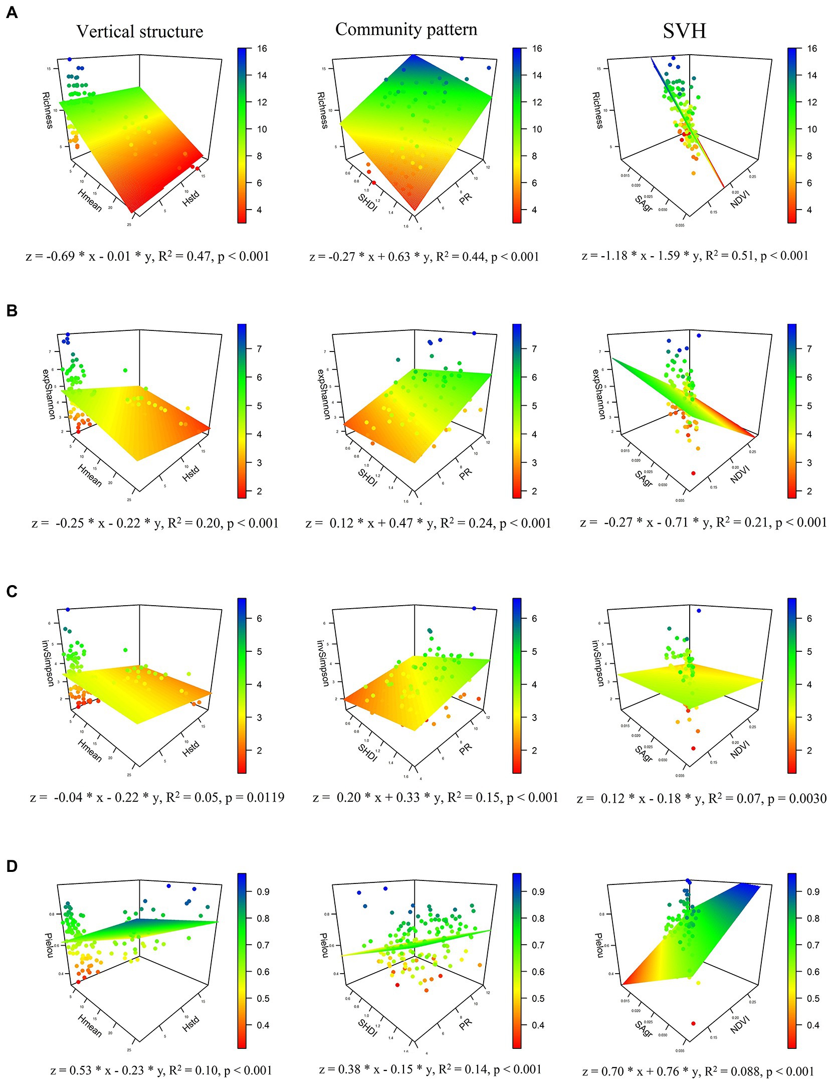
Figure 7. Scatter 3D map plotting α-diversity metrics against vertical structure, community pattern, and SVH across study sites. Vertical structure panel A–D shows the vertical structure predictor, with Hmean and Hstd as x and y, respectively; Community pattern panel A–D shows the community pattern predictor, with SHDI and PR as x and y, respectively; SVH panel A–D shows the spectral predictor, with SAgr and NDVI as x and y, respectively. The z-axis represents the α-diversity metric of species richness (A), expShannon (B), invSimpson (C), and Pielou (D) indices. The surface was fitted using a linear regression model, and the formulas of models with the standardized coefficients are presented with R2 and value of p.
By integrating three categorized variables using SEM, the explanations were improved by 5, 1, and 14% for species richness, the expShannon, and Pielou indices, respectively (Figure 8). As with the negative relationship between richness and Pielou index (Figure 5), the SHDI variable showed a strongly opposite response to species richness compared to the Pielou index (rp = −0.20 versus 0.33), but a diminished relationship was observed in both the expShannon and invSimpson indices (rp = 0.14 and 0.21) in the category of community pattern. As for the vertical structure category, Hmean and Hstd achieved the highest path coefficient with species richness and evenness (rp = −0.97 and 0.72). Meanwhile, similar situations with asymmetrical and disproportional relationships among these four metrics were observed (−0.97 < rp < 0.72). In contrast, NDVI in the SVH category showed moderate performance in explaining variation in the four metrics of α-diversity. As for the interplay of three categorized variables per se, we found that NDVI was strongly dependent on vertical structure (rp = 0.87). Variation in R2, which ranged from 0.13 to 0.56, indicated that the responses of the explanatory variables were inconsistent and mirrored the complexity of the α-diversity description. Overall, the variation in species richness and Pielou index (R2 = 0.56 and 0.28) were modeled better by SEM than the expShannon and invSimpson indices were (R2 = 0.25 and 0.13).
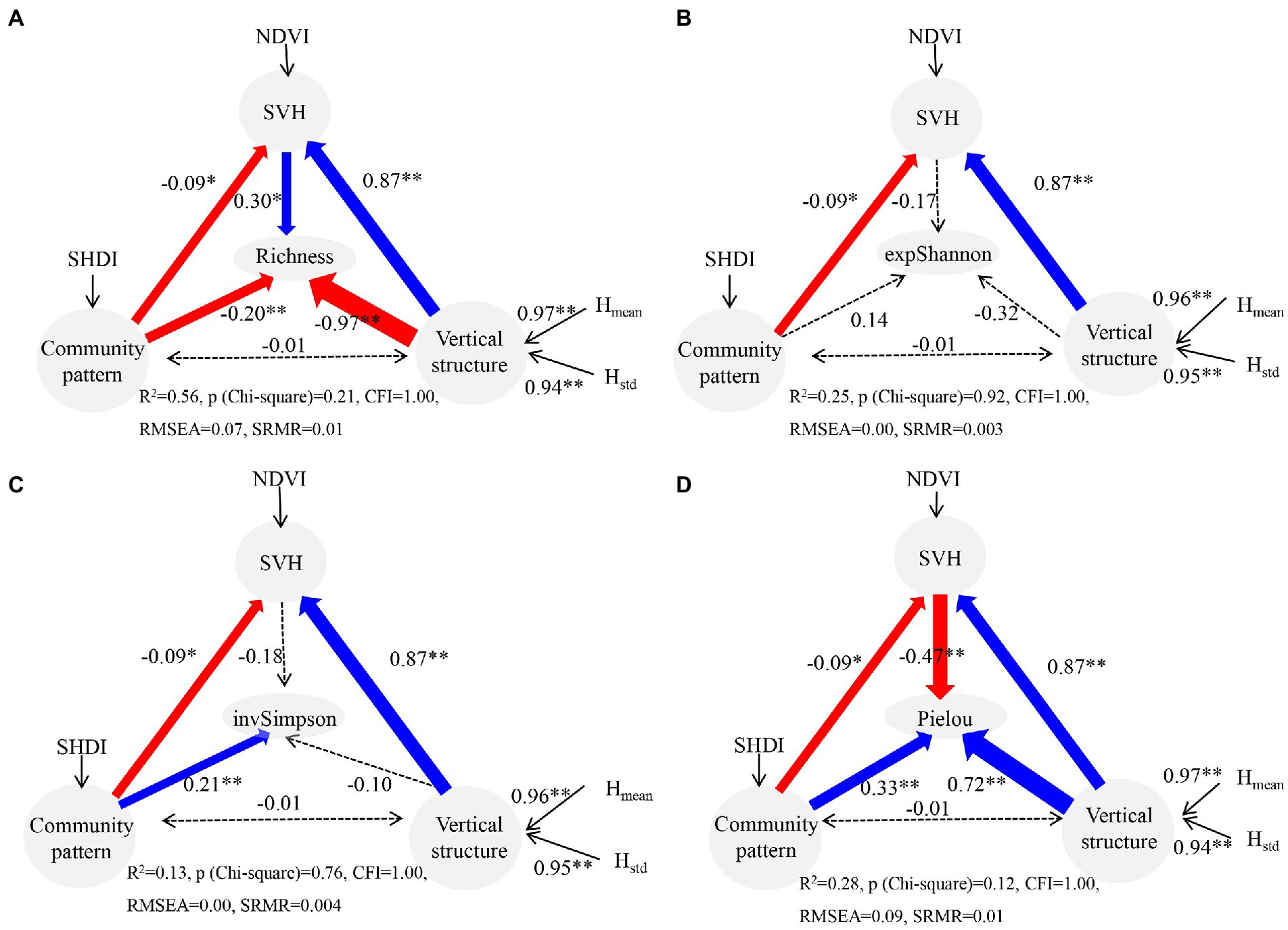
Figure 8. SEMs for four α-diversity metrics across three steppes. (A) Species richness, (B) expShannon index, (C) invSimpson index, and (D) Pielou index. Solid blue and red single-headed arrows indicate significant positive and negative effects (p < 0.05), respectively. The dashed black arrows indicate insignificant effects (p > 0.05), and the number of asterisks (*) indicates an increasing level of statistical significance from p < 0.05 to 0.01.
Precipitation has been demonstrated to be a dominant environmental factor influencing the species diversity of grassland ecosystems by promoting species richness, heterogeneity, evenness, functional divergence, and biomass (Kang et al., 2007; Reynaert et al., 2021). However, species are idiosyncratic and highly depend on their local plant community in their response to precipitation variation across various heterogeneous patches and niches (Tsafack et al., 2021). This exposes the intrinsic complication in predicting how grassland communities respond to climatic change (Barnett and Facey, 2016). Up from the prior meteorological observations of 2010–2019, the precipitation in 2020 increased by 30.96% in TS and 22.18% in DS (Figure 9A). As a result, the proportion of annual species increased by 27.27 and 28.57% (Figure 9B), respectively. This strong and disproportional response of annual species to precipitation fluctuation between TS and DS bloated species richness and the expShannon index to abnormally high levels. This scenario was especially promising in DS, resulting in higher species richness, expShannon, and invSimpson in DS compared to TS. The same process also occurred in the abundance of dominant species for TS and DS (Figure 9B). The concurrent increases in annual species and abundance of dominant species led to evenness (i.e., Pielou index) declining, emerging the negative relationship between species richness and evenness in TS. The differing sensitivity of species diversity to precipitation fluctuation in DS and TS and the adverse variations in species richness and evenness highlight the complexity and variability of α-diversity in response to climate change (Zhang et al., 2014).

Figure 9. Effects of precipitation variation on community species composition across the three steppes. (A) Precipitation and its percent variation in 2020 relative to the prior period 2010–2019. (B) The abundance of dominant species and percentage of annual species. The error bars indicate the standard deviation.
Consistently, MacDonald et al. (2017) also noted asymmetric variation in α-diversity in response to annual precipitation and the growing season temperature, and this resulted in an increased abundance of rare species as well as a disproportionally increased abundance of common species. These cases demonstrate the prevalence of the effect of environmental change on the pattern of α-diversity (Kang et al., 2007; Wilsey and Stirling, 2007; Smith et al., 2022). In contrast to precipitation increases in TS and DS, annual species were constrained in MS due to declining precipitation (4.80% decrease), which aligned with the significantly reduced aboveground biomass (AGB) (>Supplementary Table S1). These above findings speak to the first objective, where the differing sensitivity of α-diversity metrics and interactive behavior between richness and evenness reflect intricate and asynchronous responses of α-diversity to precipitation variation across various heterogeneous patches and niches. In addition, herbivores tend to prefer perennial and tall plants to annual and short plants (Díaz et al., 2007), which accordingly leads to a decrease in the abundance of perennial forbs but is insignificant for the perennial bunchgrasses (Liang et al., 2018). When precipitation is in short supply, increased consumption of net primary production by grazing herbivores aggravates the community more strongly (Liang et al., 2018). However, due to the lack of investigation on grazing practices over the region, we are limited in our ability to examine the integrated effects of grazing on variation in species diversity.
The community pattern can be conceptualized as a horizontal space that individual plant emergence, aggregation, and the physical arrangement relevant to resource facilitation and/or competition (Wesuls et al., 2013). Based on the empirical regression and SEM analysis (Figures 7, 8), we found that the community pattern significantly correlated with species richness, invSimpson, and Pielou indices. In contrast, vertical structure partly reflected the variation in species diversity because of the height heterogeneity existing among species (Torresani et al., 2020). The underperformance of vertical structure can be inferred to the grazing impact of large herbivores, which leads to a homogeneous plant height and then constrain the effort on differentiating α-diversity variation (Zhu et al., 2012). SVH has been widely used to detect plant biodiversity in a broad range of ecosystems, primarily by linking spectral properties to species and habitat distribution (Wang and Gamon, 2019). Currently, spectral variation is utilized to identify the plant functional group related to plant light absorption, and scattering is used to detect plant spectral properties (Cavender-Bares et al., 2017). In addition, the grassland community composition (e.g., species richness, evenness) can be sensitive to spectral variation, indicating that species richness and evenness together yield a more robust SVH relative to either diversity metric alone (Wang et al., 2018). Here, we found that SVH variables only explained 21 and 7% of the variation in the expShannon and invSimpson indices (Figures 7B,C). This weak explanation was attributed to the strong collinearity with properties of community pattern and vertical structure, which led to the insensitivity of spectral recognition. Accordingly, we questioned the value of exclusively using SVH to model α-diversity metrics. Additional factors for determining SVH are considerably constrained by atmospheric influence (Myneni and Asrar, 1994), limitations of spatial and spectral resolution (Bannari et al., 2002), the influence of topography (Zarnetske et al., 2019), soil background and the nature of optical saturation (Aneece et al., 2017). Altogether, the many limitations of SVH signify the caution of using SVH to explain α-diversity variation. This speaks to the last two objectives, where overall asynchronous variations in α-diversity metrics due to precipitation variation result in the asymmetric performance of the three categorized explanatory variables, thus demonstrating the limitations of using SVH to model variation in α-diversity metrics.
The common mission to depict the number of species and their relative abundances across different scales and biomes has led to the creation of multiple metrics of species diversity (Pielou, 1966; Hill, 1973). Among α-diversity metrics, the Hill numbers were meant to characterize α-diversity by focusing on the abundance of rare and common species (Chao et al., 2014; Roswell et al., 2021). A robust explanation of the expShannon and invSimpson indices is shown in Table 3, as a linear function of species richness and evenness, with uniform positive regression coefficients achieved over the region. MacDonald et al. (2017) suggested that coupling species richness with evenness can broaden the knowledge of the trends of fluctuating species diversity. However, we emphasize that the negative correlation between species richness and evenness led to unpredictable and inconsistent interpretations of α-diversity variation in the resulting models. Furthermore, richness in TS strongly affected the variation in the expShannon and invSimpson indices, while evenness in MS and DS contributed more to the variation in the expShannon and invSimpson indices (Table 3). This means that drawing out the distinctions between α-diversity metrics can be paramount for improving the performance of the integrated SEM scheme for depicting α-diversity variation, regardless of various heterogeneous patches and niches.

Table 3. The normalized regression coefficients of two independent variables (species richness and evenness) are linearly related to individual expShannon and invSimpson indices, where the linear regression was repeatedly conducted on the three steppes (i.e., MS, TS, and DS).
Climate change and anthropogenic activity have led to precipitous biodiversity loss and rampant variation in biodiversity distribution and composition (Ryabov et al., 2022), affecting the underlying mechanisms of biodiversity variation (Wilsey et al., 2005). Local species loss averages up to 14% (Newbold et al., 2015), while globally, over 20% of vascular plant species face severe threat of extinction (Schweiger et al., 2018). These losses have raised concerns about the consequential changes in ecosystem functioning and services, including nutrient cycling, climate regulation, and food production (Qiu and Cardinale, 2020). The accelerating declines in wild species and the complexity of the involved dynamics have sparked a concerted effort to answer the question about the distribution of biodiversity and the identification of high-priority areas for conservation to maintain essential ecosystem functioning and services (Wang and Gamon, 2019).
Airborne remote sensing techniques are widely utilized by scientific communities to model biodiversity variation (Coops et al., 2021). A solid method is needed for monitoring biodiversity variation over temporal and spatial scales. However, the existing theories that have been proposed based on spectral variation are still limited in addressing these issues. Ultra-resolution data portrayed by high-resolution airborne satellites (e.g., worldview 3) or unmanned aerial vehicles (UAVs) offer more information, reflecting subtle properties in plants (Wang and Gamon, 2019). State-of-the-art machine learning algorithms, such as support vector machine classification (SVM) and decision tree models, have been widely used to explore this data, and desirable results have been achieved (Delalieux et al., 2012; Lopatin et al., 2017). Meanwhile, high-density point clouds, scanned using the emerging technology of Light Detection and Ranging (LiDAR), are used for phenotypic property inversion through three-dimensional reconstructions (Sankey et al., 2021). Successful applications have emerged in forest ecosystems with species diversity detection by height heterogeneity (Marselis et al., 2020; Torresani et al., 2020), but applications in grazing ecosystems are still nascent. To understand the responding and interactive mechanism of these biodiversity metrics to climate change, it will be necessary to expand investigations into a heterogeneous grassland ecosystem (Gholizadeh et al., 2022). Further, grazing practices imposed by humans are another factor that should be assessed. The theoretical SEM proposed in this study is expected to combine emerging methods and techniques in a way that sheds light on biodiversity variation in various grassland ecosystems, coexisting with the above two forcing scenarios.
To identify the underlying interactions between α-diversity metrics and their influence on the modeling of α-diversity variation, 16 physical variables categorized into three perspectives (i.e., community pattern, vertical structure, and SVH) were used to model α-diversity variation in meadow, typical and desert steppes. We found that species richness (increase) and evenness (decline) have a strong negative response to precipitation variation in the typical steppe. An increase in annual species and a shift in the abundance of the dominant species, which are both associated with precipitation variation, are responsible for the negative relationship that we observed. More importantly, we found that the modeling of expShannon and invSimpson indices over the region was substantially influenced by the negative relationship, evidenced by a diminished ability to deploy SEM. Overall, community pattern variables explained the variation in species richness, invSimpson, and Pielou indices well, whereas SVH variables were more limited due to the strong collinearity with the properties of community pattern and vertical structure. This study emphasizes the substantial impact of the variability of α-diversity metrics in response to environmental change on the modeling of α-diversity variation over heterogeneous ecosystems.
The original contributions presented in the study are included in the article/Supplementary material, further inquiries can be directed to the corresponding author.
HY contributed to the investigation, formal analysis, and original draft. FL contributed to conceptualization, manuscript revision, and funding acquisition. GL contributed to the manuscript revision. All authors contributed to the article and approved the submitted version.
This work was supported by the Natural Science Foundation of Inner Mongolia Autonomous Region (2021SHZR1945), the Open Research Fund of Key Laboratory of Digital Earth Science, the Institute of Remote Sensing and Digital Earth, Chinese Academy of Sciences (2020LDE005), and the Agricultural Science and Technology Innovation Program of CAAS (CAAS-ASTIP-2020-IGR-04).
We thank Joseph Elliot at the University of Kansas for his technical editing work on this manuscript.
The authors declare that the research was conducted in the absence of any commercial or financial relationships that could be construed as a potential conflict of interest.
All claims expressed in this article are solely those of the authors and do not necessarily represent those of their affiliated organizations, or those of the publisher, the editors and the reviewers. Any product that may be evaluated in this article, or claim that may be made by its manufacturer, is not guaranteed or endorsed by the publisher.
The Supplementary material for this article can be found online at: https://www.frontiersin.org/articles/10.3389/fevo.2023.1108739/full#supplementary-material
Aneece, I. P., Epstein, H., and Lerdau, M. (2017). Correlating species and spectral diversities using hyperspectral remote sensing in early-successional fields. Ecol. Evol. 7, 3475–3488. doi: 10.1002/ece3.2876
Bai, Y., Wu, J., Xing, Q., Pan, Q., Huang, J., Yang, D., et al. (2008). Primary production and rain use efficiency across a precipitation gradient on the Mongolia plateau. Ecology 89, 2140–2153. doi: 10.1890/07-0992.1
Bannari, A., Asalhi, H., and Teillet, P. M. (2002). Transformed difference vegetation index (TDVI) for vegetation cover mapping. IEEE International geoscience and remote sensing symposium. Toronto, ON, Canada, 3053–3055.
Barnett, K. L., and Facey, S. L. (2016). Grasslands, invertebrates, and precipitation: a review of the effects of climate change. Front. Plant Sci. 7:1196. doi: 10.3389/fpls.2016.01196
Cavender-Bares, J., Gamon, J. A., Hobbie, S. E., Madritch, M. D., Meireles, J. E., Schweiger, A. K., et al. (2017). Harnessing plant spectra to integrate the biodiversity sciences across biological and spatial scales. Am. J. Bot. 104, 966–969. doi: 10.3732/ajb.1700061
Chao, A. N., Chiu, C. H., and Jost, L. (2014). Unifying species diversity, phylogenetic diversity, functional diversity, and related similarity and differentiation measures through Hill numbers. Annu. Rev. Ecol. Evol. S 45, 297–324. doi: 10.1146/annurev-ecolsys-120213-091540
Chesson, P. (2000). Mechanisms of maintenance of species diversity. Annu. Rev. Ecol. Syst. 31, 343–366. doi: 10.1146/annurev.ecolsys.31.1.343
Cleland, E. E., Collins, S. L., Dickson, T. L., Farrer, E. C., Gross, K. L., Gherardi, L. A., et al. (2013). Sensitivity of grassland plant community composition to spatial vs. temporal variation in precipitation. Ecology 94, 1687–1696. doi: 10.1890/12-1006.1
Coops, N. C., Tompalski, P., Goodbody, T. R. H., Queinnec, M., Luther, J. E., Bolton, D. K., et al. (2021). Modelling lidar-derived estimates of forest attributes over space and time: a review of approaches and future trends. Remote Sens. Environ. 260:112477. doi: 10.1016/j.rse.2021.112477
Currie, D. J., Mittelbach, G. G., Cornell, H. V., Field, R., Guegan, J. F., Hawkins, B. A., et al. (2004). Predictions and tests of climate-based hypotheses of broad-scale variation in taxonomic richness. Ecol. Lett. 7, 1121–1134. doi: 10.1111/j.1461-0248.2004.00671.x
DeJong, T. M. (1975). A comparison of three diversity indices based on their components of richness and evenness. Oikos 26, 222–227. doi: 10.2307/3543712
Delalieux, S., Somers, B., Haest, B., Spanhove, T., Borre, J. V., and Mücher, C. (2012). Heathland conservation status mapping through integration of hyperspectral mixture analysis and decision tree classifiers. Remote Sens. Environ. 126, 222–231. doi: 10.1016/j.rse.2012.08.029
Díaz, S., Lavorel, S., McIntyre, S., Falczuk, V., Casanoves, F., Milchunas, D. G., et al. (2007). Plant trait responses to grazing–a global synthesis. Glob. Change Biol. 13, 313–341. doi: 10.1111/j.1365-2486.2006.01288.x
Fauvel, M., Lopes, M., Dubo, T., Rivers-Moore, J., Frison, P. L., Gross, N., et al. (2020). Prediction of plant diversity in grasslands using Sentinel-1 and-2 satellite image time series. Remote Sens. Environ. 237:111536. doi: 10.1016/j.rse.2019.111536
Gholizadeh, H., Dixon, A. P., Pan, K. H., McMillan, N. A., Hamilton, R. G., Fuhlendorf, S. D., et al. (2022). Using airborne and DESIS imaging spectroscopy to map plant diversity across the largest contiguous tract of tallgrass prairie on earth. Remote Sens. Environ. 281:113254. doi: 10.1016/j.rse.2022.113254
Golodets, C., Kigel, J., and Sternberg, M. (2011). Plant diversity partitioning in grazed Mediterranean grassland at multiple spatial and temporal scales. J. Appl. Ecol. 48, 1260–1268. doi: 10.1111/j.1365-2664.2011.02031.x
Hauser, L. T., Timmermans, J., van der Windt, N., Sil, Â. F., César de Sá, N., Soudzilovskaia, N. A., et al. (2021). Explaining discrepancies between spectral and in-situ plant diversity in multispectral satellite earth observation. Remote Sens. Environ. 265:112684. doi: 10.1016/j.rse.2021.112684
Hijmans, R. J. (2022). Raster: Geographic Data Analysis and Modeling. R package version 3.6-11. Available at: https://CRAN.R-project.org/package=raster
Hill, M. (1973). Diversity and evenness: a unifying notation and its consequences. Ecology 54, 427–432. doi: 10.2307/1934352
Hooper, D., Coughlan, J., and Mullen, M. R. (2008). Structural equation modelling: Guidelines for determining model fit. Electron. J. Bus. Res. Methods 6, 53–60.
Kang, L., Han, X. G., Zhang, Z. B., and Sun, O. J. (2007). Grassland ecosystems in China: review of current knowledge and research advancement. Philos. Trans. R. Soc. Lond. Ser. B Biol. Sci. 362, 997–1008. doi: 10.1098/rstb.2007.2029
Kardol, P., Campany, C. E., Souza, L., Norby, R. J., Weltzin, J. F., and Classen, A. T. (2010). Climate change effects on plant biomass alter dominance patterns and community evenness in an experimental old-field ecosystem. Glob. Change Biol. 16, 2676–2687. doi: 10.1111/j.1365-2486.2010.02162.x
Liang, M., Chen, J., Gornish, E. S., Bai, X., Li, Z., and Liang, C. (2018). Grazing effect on grasslands escalated by abnormal precipitations in Inner Mongolia. Ecol. Evol. 8, 8187–8196. doi: 10.1002/ece3.4331
Liu, G., Xie, X., Ye, D., Ye, X., Tuvshintogtokh, I., Mandakh, B., et al. (2013). Plant functional diversity and species diversity in the Mongolian steppe. PLoS One 8:e77565. doi: 10.1371/journal.pone.0077565
Lopatin, J., Fassnacht, F. E., Kattenborn, T., and Schmidtlein, S. (2017). Mapping plant species in mixed grassland communities using close range imaging spectroscopy. Remote Sens. Environ. 201, 12–23. doi: 10.1016/j.rse.2017.08.031
Loreau, M. (2000). Biodiversity and ecosystem functioning: recent theoretical advances. Oikos 91, 3–17. doi: 10.1034/j.1600-0706.2000.910101.x
MacDonald, Z. G., Nielsen, S. E., and Acorn, J. H. (2017). Negative relationships between species richness and evenness render common diversity indices inadequate for assessing long-term trends in butterfly diversity. Biodivers. Conserv. 26, 617–629. doi: 10.1007/s10531-016-1261-0
Marcinkowska-Ochtyra, A., Jarocińska, A., Bzdęga, K., and Tokarska-Guzik, B. (2018). Classification of expansive grassland species in different growth stages based on hyperspectral and LiDAR data. Remote Sens. 10:2019. doi: 10.3390/rs10122019
Marselis, S. M., Abernethy, K., Alonso, A., Armston, J., Baker, T. R., Bastin, J. F., et al. (2020). Evaluating the potential of full-waveform lidar for mapping pan-tropical tree species richness. Glob. Ecol. Biogeogr. 29, 1799–1816. doi: 10.1111/geb.13158
McCann, K. S., Rasmussen, J. B., and Umbanhowar, J. (2005). The dynamics of spatially coupled food webs. Ecol. Lett. 8, 513–523. doi: 10.1111/j.1461-0248.2005.00742.x
McGarigal, K., and Marks, B. J. (1995). FRAGSTATS: spatial pattern analysis program for quantifying landscape structure. US Department of Agriculture, Forest Service, Pacific Northwest Research Station. Available at: www.fs.usda.gov/treesearch/pubs/3064
Myneni, R., and Asrar, G. (1994). Atmospheric effects and spectral vegetation indices. Remote Sens. Environ. 47, 390–402. doi: 10.1016/0034-4257(94)90106-6
Navarrete, S. A., and Berlow, E. L. (2006). Variable interaction strengths stabilize marine community pattern. Ecol. Lett. 9, 526–536. doi: 10.1111/j.1461-0248.2006.00899.x
Newbold, T., Hudson, L. N., Hill, S. L., Contu, S., Lysenko, I., Senior, R. A., et al. (2015). Global effects of land use on local terrestrial biodiversity. Nature 520, 45–50. doi: 10.1038/nature14324
Oksanen, J., Simpson, G., Blanchet, F., Kindt, R., Legendre, P., Minchin, P., et al. (2022). Vegan: Community Ecology Package. R package version 2.6-4, Available at: https://CRAN.R-project.org/package=vegan
Palmer, M. W., Earls, P. G., Hoagland, B. W., White, P. S., and Wohlgemuth, T. (2002). Quantitative tools for perfecting species lists. Environmetrics 13, 121–137. doi: 10.1002/env.516
Petermann, J. S., and Buzhdygan, O. Y. (2021). Grassland biodiversity. Curr. Biol. 31, R1195–R1201. doi: 10.1016/j.cub.2021.06.060
Pielou, E. C. (1966). Species-diversity and pattern-diversity in the study of ecological succession. J. Theor. Biol. 10, 370–383. doi: 10.1016/0022-5193(66)90133-0
Qiu, J., and Cardinale, B. J. (2020). Scaling up biodiversity-ecosystem function relationships across space and over time. Ecology 101:3166. doi: 10.1002/ecy.3166
Questad, E. J., and Foster, B. L. (2008). Coexistence through spatio-temporal heterogeneity and species sorting in grassland plant communities. Ecol. Lett. 11, 717–726. doi: 10.1111/j.1461-0248.2008.01186.x
R Core Team. (2022). R: A language and environment for statistical computing. R Foundation for Statistical Computing, Vienna, Austria. Available at: https://www.R-project.org/
Reynaert, S., De Boeck, H. J., Verbruggen, E., Verlinden, M., Flowers, N., and Nijs, I. (2021). Risk of short-term biodiversity loss under more persistent precipitation regimes. Glob. Change Biol. 27, 1614–1626. doi: 10.1111/gcb.15501
Rosseel, Y. (2012). Lavaan: an R package for structural equation modeling. J. Stat. Softw. 48, 1–36. doi: 10.18637/jss.v048.i02
Roswell, M., Dushoff, J., and Winfree, R. (2021). A conceptual guide to measuring species diversity. Oikos 130, 321–338. doi: 10.1111/oik.07202
Ryabov, A., Blasius, B., Hillebrand, H., Olenina, I., and Gross, T. (2022). Estimation of functional diversity and species traits from ecological monitoring data. Proc. Natl. Acad. Sci. U. S. A. 119:e2118156119. doi: 10.1073/pnas.2118156119
Sankey, J. B., Sankey, T. T., Li, J., Ravi, S., Wang, G., Caster, J., et al. (2021). Quantifying plant-soil-nutrient dynamics in rangelands: fusion of UAV hyperspectral-LiDAR, UAV multispectral-photogrammetry, and ground-based LiDAR-digital photography in a shrub-encroached desert grassland. Remote Sens. Environ. 253:112223. doi: 10.1016/j.rse.2020.112223
Schmidtlein, S., and Fassnacht, F. E. (2017). The spectral variability hypothesis does not hold across landscapes. Remote Sens. Environ. 192, 114–125. doi: 10.1016/j.rse.2017.01.036
Schweiger, A. K., Cavender-Bares, J., Townsend, P. A., Hobbie, S. E., Madritch, M. D., Wang, R., et al. (2018). Plant spectral diversity integrates functional and phylogenetic components of biodiversity and predicts ecosystem function. Nat. Ecol. Evol. 2, 976–982. doi: 10.1038/s41559-018-0551-1
Smith, M. D., Koerner, S. E., Avolio, M. L., Komatsu, K. J., Eby, S., Forrestel, E. J., et al. (2022). Richness, not evenness, varies across water availability gradients in grassy biomes on five continents. Oecologia 199, 649–659. doi: 10.1007/s00442-022-05208-6
Stirling, G., and Wilsey, B. (2001). Empirical relationships between species richness, evenness, and proportional diversity. Am. Nat. 158, 286–299. doi: 10.1086/321317
Sugita, M., Asanuma, J., Tsujimura, M., Mariko, S., Lu, M., Kimura, F., et al. (2007). An overview of the rangelands atmosphere-hydrosphere-biosphere interaction study experiment in northeastern Asia (RAISE). J. Hydrol. 333, 3–20. doi: 10.1016/j.jhydrol.2006.07.032
Thornley, R., Gerard, F. F., White, K., and Verhoef, A. (2022). Intra-annual taxonomic and phenological drivers of spectral variance in grasslands. Remote Sens. Environ. 271:112908. doi: 10.1016/j.rse.2022.112908
Torresani, M., Rocchini, D., Sonnenschein, R., Zebisch, M., Hauffe, H. C., Heym, M., et al. (2020). Height variation hypothesis: a new approach for estimating forest species diversity with CHM LiDAR data. Ecol. Indic. 117:106520. doi: 10.1016/j.ecolind.2020.106520
Tsafack, N., Borges, P. A., Xie, Y., Wang, X., and Fattorini, S. (2021). Emergent rarity properties in carabid communities from Chinese steppes with different climatic conditions. Front. Ecol. Evol. 9:250:3436. doi: 10.3389/fevo.2021.603436
Wang, R., and Gamon, J. A. (2019). Remote sensing of terrestrial plant biodiversity. Remote Sens. Environ. 231:111218. doi: 10.1016/j.rse.2019.111218
Wang, R., Gamon, J. A., and Cavender-Bares, J. (2022). Seasonal patterns of spectral diversity at leaf and canopy scales in the Cedar Creek prairie biodiversity experiment. Remote Sens. Environ 280:113169:113169. doi: 10.1016/j.rse.2022.113169
Wang, R., Gamon, J. A., Cavender-Bares, J., Townsend, P. A., and Zygielbaum, A. I. (2018). The spatial sensitivity of the spectral diversity-biodiversity relationship: an experimental test in a prairie grassland. Ecol. Appl. 28, 541–556. doi: 10.1002/eap.1669
Wang, S. P., Loreau, M., de Mazancourt, C., Isbell, F., Beierkuhnlein, C., Connolly, J., et al. (2021). Biotic homogenization destabilizes ecosystem functioning by decreasing spatial asynchrony. Ecology 102:10. doi: 10.1002/ecy.3332
Wesuls, D., Pellowski, M., Suchrow, S., Oldeland, J., Jansen, F., and Dengler, J. (2013). The grazing fingerprint: modelling species responses and trait patterns along grazing gradients in semi-arid Namibian rangelands. Ecol. Indic. 27, 61–70. doi: 10.1016/j.ecolind.2012.11.008
Whittaker, R. H. (1960). Vegetation of the Siskiyou mountains, Oregon and California. Ecol. Monogr. 30, 279–338. doi: 10.2307/1943563
Wilsey, B. J., Chalcraft, D. R., Bowles, C. M., and Willig, M. R. (2005). Relationships among indices suggest that richness is an incomplete surrogate for grassland biodiversity. Ecology 86, 1178–1184. doi: 10.1890/04-0394
Wilsey, B., and Stirling, G. (2007). Species richness and evenness respond in a different manner to propagule density in developing prairie microcosm communities. Plant Ecol. 190, 259–273. doi: 10.1007/s11258-006-9206-4
Xu, K., Su, Y., Liu, J., Hu, T., Jin, S., Ma, Q., et al. (2020). Estimation of degraded grassland aboveground biomass using machine learning methods from terrestrial laser scanning data. Ecol. Indic. 108:105747:105747. doi: 10.1016/j.ecolind.2019.105747
Zarnetske, P. L., Read, Q. D., Record, S., Gaddis, K. D., Pau, S., Hobi, M. L., et al. (2019). Towards connecting biodiversity and geodiversity across scales with satellite remote sensing. Glob. Ecol. Biogeogr. 28, 548–556. doi: 10.1111/geb.12887
Zhang, Q., Hou, X., Li, F. Y., Niu, J., Zhou, Y., Ding, Y., et al. (2014). Alpha, beta and gamma diversity differ in response to precipitation in the Inner Mongolia grassland. PLoS One 9:e93518. doi: 10.1371/journal.pone.0093518
Zhang, H., John, R., Peng, Z., Yuan, J., Chu, C., Du, G., et al. (2012). The relationship between species richness and evenness in plant communities along a successional gradient: a study from sub-alpine meadows of the eastern Qinghai-Tibetan plateau, China. PloS One 7:e49024. doi: 10.1371/journal.pone.0049024
Keywords: grasslands, α-diversity, spectral variation hypothesis, community pattern, vertical structure
Citation: Yan H, Li F and Liu G (2023) Diminishing influence of negative relationship between species richness and evenness on the modeling of grassland α-diversity metrics. Front. Ecol. Evol. 11:1108739. doi: 10.3389/fevo.2023.1108739
Received: 06 December 2022; Accepted: 10 February 2023;
Published: 03 March 2023.
Edited by:
Paulo A. V. Borges, University of the Azores, PortugalReviewed by:
Jinlong Zhang, Kadoorie Farm and Botanic Garden, Hong Kong SAR, ChinaCopyright © 2023 Yan, Li and Liu. This is an open-access article distributed under the terms of the Creative Commons Attribution License (CC BY). The use, distribution or reproduction in other forums is permitted, provided the original author(s) and the copyright owner(s) are credited and that the original publication in this journal is cited, in accordance with accepted academic practice. No use, distribution or reproduction is permitted which does not comply with these terms.
*Correspondence: Fei Li, bGlmZWkwMUBjYWFzLmNu
Disclaimer: All claims expressed in this article are solely those of the authors and do not necessarily represent those of their affiliated organizations, or those of the publisher, the editors and the reviewers. Any product that may be evaluated in this article or claim that may be made by its manufacturer is not guaranteed or endorsed by the publisher.
Research integrity at Frontiers

Learn more about the work of our research integrity team to safeguard the quality of each article we publish.