Unraveling spatiotemporal patterns and multiple driving factors of surface ozone across China and its urban agglomerations management strategies

Since State Council launched the Action Plan for Air Pollution Prevention and Control in 2013, national concentration of fine particulate matter (PM_2.5) has continued to decline in China, while surface ozone (O₃) pollution shows an obvious rise. To identity hot regions and develop targeted policy, the spatiotemporal O₃ variation and its population-weighted exposure features were analyzed in 337 cities across China, using autocorrelation analysis and grid exposure calculation. In the identified hot urban agglomerations, the correlation analysis and geographic weighted regression model (GWR) were used to study related meteorological factors and socioeconomic driving factors. O₃ pollution and its human exposure were found to have significant spatial aggregation characteristics, showing a need for regional management policy. Beijing-Tianjin-Hebei Urban Agglomeration (BTH-UA), Central Plains Urban Agglomeration (CP-UA), and Yangtze River Delta Urban Agglomeration (YRD-UA) were identified as hot regions where O₃ concentration exceeded 160 μg·m⁻³, exceedance rate was over 20% and population-weighted exposure risk was relatively high. Correlation analysis in the hot regions indicated high surface temperature, low relative humidity, and low wind speed were positive to O₃ increase. Further, GWR results revealed that O₃ in the majority of cities was positively related with population density (PD), the per capita GDP (Per_GDP), industrial soot emissions (ISE), industrial SO₂ emissions (ISO₂), and average annual concentration of inhaled fine particulate matter (PM₁₀), and negatively related with total land area of administrative region (Administration) and area of green land (Green). From the regional driving factor difference, the targeted UA management policy was provided.

1. Introduction

Since the implementation of the Action Plan for Air Pollution Prevention and Control in 2013, China’s environmental air quality has achieved remarkable results. Among the six major air pollutants, fine particulate matter (PM_2.5), coarse particulate matter (PM₁₀), sulfur dioxide (SO₂), nitrogen dioxide (NO₂), and carbon monoxide (CO) concentrations decreased significantly (Qu et al., 2020). Compared with 2014, the average annual concentration of PM_2.5, PM₁₀, SO₂, and NO₂ in 2015 decreased by 14.1, 11.4, 21.9, and 7.1%, respectively [Ministry of Ecology and Environment of the People’s Republic of China (MEE-PRC), 2016]. While the ozone (O₃) pollution prevention and control situation is gradually grim (Ziemke et al., 2019; Zhao et al., 2020), the 90th percentile concentration of average of O₃ daily maximum 8-h in 2015 increased by 3.4% compared with 2014 [Ministry of Ecology and Environment of the People’s Republic of China (MEE-PRC), 2016]. And from 2015 to 2019, among the O₃ exceedance days in 337 cities, the proportion of moderate and pollution above increased from 7.2 to 11.4% (Yan et al., 2020). With enhancement of public awareness on environmental health and requirements of high quality urban development, O₃ pollution has become the focus of the 14th Five-Year Plan governance, and it is also one of the key factors to test the success of the war to protect the blue sky. As a kind of greenhouse gas, surface O₃ will produce a series of negative effects when it continuously increases in the troposphere, such as damaging human health (Liu et al., 2018), causing serious harm to the ecological environment (Karlsson et al., 2017; Harmens et al., 2018; Li et al., 2018), etc.

Currently, the study regions of existing O₃ pollution researches were mainly limited to certain administrative divisions or some regions of interest in China (Cheng et al., 2018; Liang et al., 2020; Yang, 2021). For example, Wei et al. (2020) applied the spatial autocorrelation analysis and geographical detector to analyze the spatial and temporal changes of the O₃ concentration in 35 cities in Northeast China from 2015 to 2018. Likewise, most studies on O₃ pollution were mainly based on the specific city clusters (Wang Z. B. et al., 2020; Zhan et al., 2021), a single city (Chen Z. Y. et al., 2019), or a single year (Liu P. F. et al., 2020), and few studies explored the multi time scale variation patterns and exposure risk of surface O₃ at a national scale or the multiple urban agglomerations. Further, for O₃ pollution driving factors, researchers firstly focused on meteorological factors (He et al., 2017; Zhou et al., 2019; Chang et al., 2021), topographic (He et al., 2021), and precursor composition (Liu H. L. et al., 2020). Meanwhile, there are many socioeconomic factors affecting the O₃ pollution level, such as population density, industrial soot, and SO₂ emissions, etc. (Wang X. L. et al., 2020). Therefore, through multi spatiotemporal scale pollution features analysis, it is of significance to carry out a multiple driving factors identification and further provide regional differentiated control countermeasures.

The major aims of this study were (i) to analyze the spatiotemporal distribution and population-weighted exposure risk feature of O₃ using ground observations data of the daily maximum 8-h sliding average surface O₃ (MDA8) from Chinese 337 cities in 2015 and 2018; (ii) to explore the relationship between meteorological factors and O₃ on seasonal scales using correlation analyses in the identified hot urban agglomerations; (iii) to further identify driving effects of sensitive socioeconomic factors and urban surface O₃ in hot urban agglomerations via the geographic weighted regression model (GWR). Finally, the joint O₃ management suggestions were developed from the perspective of urban agglomeration.

2. Materials and methods

2.1. Data sources

The O₃ concentration data were derived from the daily values of urban surface O₃ concentration monitoring released by the Ministry of Ecology and Environment of the People’s Republic of China in 2015 and 2018. Compared with 2014, the average concentration of O₃ and the proportion of days exceeding the standard both increased in 2015 [Ministry of Ecology and Environment of the People’s Republic of China (MEE-PRC), 2016], and the end of Action Plan for Air Pollution Prevention and Control in 2017 and the first year of the Blue Sky Protection Campaign in 2018, so 2015 and 2018 was chosen as the study years of this paper. The study areas were 337 cities of Chinese mainland, including 333 prefecture-level cities and 4 municipalities. According to the Environmental Air Quality Standard (GB3095-2012) issued by the MEE-PRC [Environmental Protection Department (EPD), 2012], the surface O₃ “daily average” concentration means the daily maximum 8-h sliding average (MDA8), and “quarterly average” means the calculated mean of each daily average concentration in a calendar season (spring is March–May, summer is June–August, fall is September–November, and winter is December, January, and February). Environmental air functional areas are divided into Class I and Class II: ① Class I consists of nature reserves, scenic spots, and other areas requiring special protection, with a limit of 100 μg·m⁻³ for MDA8 concentration; ② Class II includes residential areas, mixed areas for commercial traffic residents, cultural areas, industrial areas, and rural areas, with a limit of 160 μg·m⁻³ for MDA8 concentration. According to the Technical Specification for Environmental Air Quality Evaluation (Trial; HJ663-2013) issued by the MEE-PRC, “Annual evaluation” is determined by the 90th percentile of average of O₃ daily maximum 8-h (MDA8-90%). The exceedance rate discussed in this study refers to the O₃ daily evaluation is the percentage of the exceedance over a certain period of time.

The related series of meteorological data, including temperature (°C), wind speed (m·s⁻¹), and relative humidity (%) were obtained from the China Meteorological Administration (http://data.Cma.cn; Liu P. F. et al., 2020; Hu et al., 2021). Further, the socioeconomic data were derived from the China Statistical Yearbook. A total of 14 related statistical metrics indicators were selected and extracted following the Delphi method and the published literature review (Huang et al., 2019; Chen et al., 2020; Wang X. L. et al., 2020; Wang et al., 2021): total population at year-end (TP), population density (PD), the gross domestic product (GDP), and the per capita GDP (Per_GDP), share of the primary industry in GDP (%; Primary), share of the secondary industry in GDP (%; Secondary), share of the tertiary industry in the GDP (%; Tertiary), industrial soot emissions (ISE), annual average population (AP), total land area of administrative region (Administration), area of green land (Green), industrial SO₂ emissions (ISO₂), average annual concentration of inhaled fine particulate matter (PM₁₀), and annual electricity consumption (AEC).

2.2. Methods

2.2.1. Global and local autocorrelation analysis

Global Moran’s I is the best known and used method to reflect the similarity of spatial adjacent or adjacent regional cell property values (Chen, 2021). Moran’s I is calculated as the following Eq. (1):

$\begin{array}{ll}I=\frac{n{\displaystyle \sum }_{i=1}^n{\displaystyle \sum }_{j=1}^n{w}_{ij}\left(x_i-\overline{x}\right)\left(x_j-\overline{x}\right)}{\left({\displaystyle \sum }_{i=1}^n{\displaystyle \sum }_{j=1}^n{w}_{ij}\right){\displaystyle \sum }_{i=1}^n{\left(x_i-\overline{x}\right)}^2}& (1)\end{array}$

where n is the number of monitoring cities; x_i and x_j refer to the attribute values of city i and j, respectively; w_ij is the spatial weight matrix between the regional units i and j.

Z_I is used to test the significance of global Moran’s I, and the calculation formula is as follows:

$\begin{array}{ll}{Z}_I=\frac{I-E_I}{\sqrt{Va{r}_I}}& (2)\end{array}$

where Z_I is the Z test value for the global Moran’s I; E_I and Var_I are the mathematical expectation and covariance of the global Moran’s I, respectively.

The global spatial autocorrelation index can only reflect the overall process or trend, while it cannot reveal local differences. Therefore, it cannot specifically reflect the correlation and correlation between a city and its neighboring city (Zhou et al., 2020). To more accurately grasp the aggregation and differentiation characteristics of O₃ spatial agglomeration, the local Moran’s I (Anselin, 2010) is presented by Eq. (3):

$\begin{array}{ll}{I}_i=\frac{{\displaystyle \sum }_{j=1}^n{w}_{ij}{x}_j-\overline{x}{\displaystyle \sum }_{j=1}^n{w}_{ij}}{S\sqrt{\frac{\left[n{\displaystyle \sum }_{j=1}^n{w}_{ij}^2-{\left({\displaystyle \sum }_{j=1}^n{w}_{ij}\right)}^2\right]}{n-1}}}& (3)\end{array}$

where S is the standard deviation; If I_i is positive and significant, the position i is hot spot (high value agglomeration), if I_i is negative and significant, the position i is cold point (low value agglomeration).

2.2.2. Exposure risk assessment methods

To more scientifically and reasonably reflect the population exposure risk of O₃ in the study area; this paper calculates the population-weighted O₃ concentration value of a single grid by using a grid calculator (Fu and Kan, 2004). The calculation formula is as follows:

$\begin{array}{ll}PWE{L}_i=\frac{P_i\times C_i}{\sum P_i}& (4)\end{array}$

where PWEL_i is the population-weighted O₃ concentration average value, μg·m⁻³; i is the number of grid cells; P_i is the number of population in the grid; C_i is the O₃ concentration in this grid/(μg·m⁻³).

2.2.3. Meteorological factors and correlation analysis

The Pearson correlation coefficient test was used to determine the correlation between the O₃ concentration and the meteorological factors (Dong et al., 2021). Correlation coefficient r can be calculated using Eq. (5):

$\begin{array}{ll}r=\frac{1}{n-1}{\displaystyle \sum }_{i=1}^n\left(\frac{X_i-\overline{X}}{S_X}\right)\left(\frac{Y_i-\overline{Y}}{S_Y}\right)& (5)\end{array}$

where X_i, Y_i are the values of two random variables X and Y with linear relations, respectively; i is the number of samples, i = 1, 2, …, n; S_X and S_Y are the standard differences of the variable X, Y, respectively.

2.2.4. Variance inflation factor

To better quantify the contribution of each socioeconomic factor to the O₃ concentration variety, the collinearity between explanatory variables should be first eliminated (Guo et al., 2016). The variance inflation factor (VIF) test is a classical method used to test the probable multicollinearity (Zhao et al., 2016; Che et al., 2019). In this study, multicollinearity was judged by statistics (T), robust probability (P), and variance inflation factor (VIF). Judgment methods were as follows: the larger the T is, the more significant the representation is; the smaller the p value is, the more useful variable is; if 0 < VIF < 10, there is no multicollinearity, and vice versa.

2.2.5. Geographic weighted regression

When establishing econometric models with cross-section data, the impact of explanatory variables on the interpreted variables may be different between regions due to the complexity, autocorrelation, and variability that this data exhibits. The GWR model can address the problem, which assumes that the economic behavior between regions is spatially heterogeneous and more realistic (Wang S. J. et al., 2020). The GWR model is as follows:

$\begin{array}{ll}{y}_j={\beta }_0\left(u_j\mathrm{,}{v}_j\right)+{\displaystyle \sum }_{i=1}^k{\beta }_i\left(u_j\mathrm{,}{v}_j\right)x_{ij}+{\epsilon }_j& (6)\end{array}$

where x, y are independent and dependent variables, respectively; k is the number of independent variables; j is sample point; ε is regression residue; β₀ (u_j, v_j) is the intercept; and β_i (u_j, v_j) is the regression coefficient, changing with the sample point location. Each local β_i (u_j, v_j) is used to estimate its adjacent spatial observations.

3. Results and discussion

3.1. Spatiotemporal distribution characteristics of O₃

3.1.1. Annual distribution characteristics

Figure 1 shows the national distribution and the daily average exceedance rate of urban MDA8-90% in 2015 and 2018. In 2015 and 2018, the average annual concentration range were 62–202 and 74–215 μg·m⁻³, with a total of 60 and 111 cities exceeding the standard value (160 μg·m⁻³), accounting for 17.8% (60/337) and 32.9% (111/337), respectively. O₃ pollution distribution showed similarity to a certain extent in 2015 and 2018 and heavily polluted area was mainly concentrated in eastern China, such as Liaoning, Shandong, Hebei, Henan, and Jiangsu. Specifically, compared with 2015, O₃ distribution was more concentrated and serious in 2018. The polluted cities in severely polluted areas increased and the polluted areas gradually spread, for example, Shanxi, Shaanxi, and Anhui also began to suffer O₃ pollution.

FIGURE 1

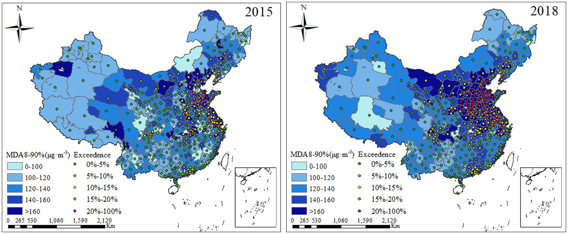
Figure 1. Spatiotemporal distribution of MDA8-90% and daily average exceedance rate in Chinese 337 cities.

As shown in the Figure 1, the areas with high O₃ exceedance rate were mainly concentrated in the eastern coastal areas of China, and it gradually spread to the central region. In 2015, the exceedance rate range of O₃ concentration was 0.00–24.93%. Among the studied 337 cities, the exceedance rates of 28 cities were above 15%, and those of four cities were above 20%, and these cities mainly located in Jiangsu, Shandong, Hebei, and Beijing. In 2018, the exceedance rate range of O₃ concentration was 0.00–30.14%, and the exceedance rates of 67 cities were above 15%, and those of 32 cities were above 20%. Generally, the Chinese O₃ concentrations and pollution area in 2018 have both increased compared with that in 2015; hence, it is of great significance to explore the spatial agglomeration and seasonal distribution characteristics.

3.1.2. Seasonal spatiotemporal distribution characteristics

Figure 2 shows the seasonal distribution of O₃ concentration in Chinese cities. Generally, the O₃ pollution in spring and summer was more serious, and the pollution scope were wider than that in fall and winter. Specifically, the high incidence areas of O₃ pollution in spring were mainly concentrated in central and eastern provinces, including Jiangsu, Shandong, Hebei, and Henan. In summer, pollution had spread to the western provinces, including Shaanxi, Gansu, Qinghai, Sichuan, and Inner Mongolia. The O₃ pollution areas decreased in fall compared with spring and summer, and these areas were mainly concentrated in Shandong, Jiangsu, and Anhui. In winter, O₃ pollution areas was mainly concentrated in the central and western provinces, including Sichuan, Qinghai, and Gansu.

FIGURE 2

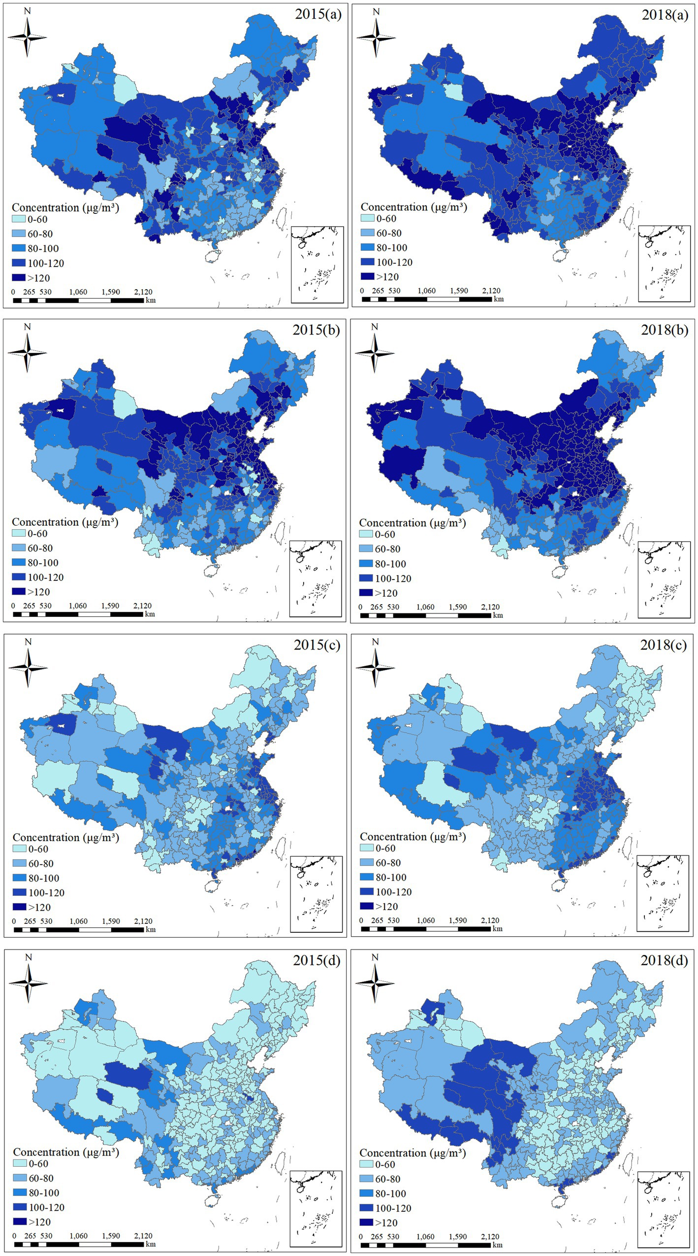
Figure 2. Seasonal spatiotemporal distribution of MDA8 in Chinese 337 cities: (A) spring, (B) summer, (C) fall, and (D) winter.

3.2. Spatial agglomeration characteristics

To explore the presence of spatial dependence in observations, ArcGIS 10.2 Desktop’s Spatial Autocorrelation Model tool was used to test the annual and quarterly data of O₃ concentration in 337 cities in 2015 and 2018, respectively. The annual and quarterly Moran’s I index were shown in Table 1. The results showed that annual Moran’s I were both above 0.00 and Z(I) exceeded 2.58, and they all passed the significance test of 0.01 level in 2015 and 2018. It indicated a significant spatial positive correlation of O₃ concentration in China. Moran’s I and Z(I) were higher in 2018 (0.72, 49.89) than those in 2015 (0.29, 20.04), which reflected the O₃ pollution was more concentrated and serious in 2018. It could be due to that the similar emission control measures were adopted by different regions, which reduced the spatial differences of O₃ precursor’s emissions in a certain extent. In addition, the seasonal characteristics of Moran’s I were also relatively obvious (summer > fall > spring and winter), which indicated that the correlation of urban O₃ in summer was the highest.

TABLE 1

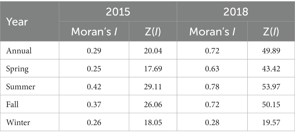
Table 1. Spatial autocorrelation index of O₃ concentration in Chinese 337 cities.

3.2.1. Annual spatial agglomeration characteristics

The annual spatial agglomeration feature of national O₃ concentration is shown in Figure 3. The distribution areas of cold and hot spots were similar in 2015 and 2018 to a certain extent, which indicated that Chinese cities have formed a relatively stable and continuous pollution area. Hot spots were mainly distributed in eastern and central provinces, including Shanghai, Jiangsu, Anhui, Shandong, Beijing, Hebei, Shanxi, and Henan. Moreover, compared with 2015, Shaanxi, Inner Mongolia, Hubei, and Zhejiang have gradually become hot agglomeration areas in 2018. Cold points were mainly distributed in Guangxi, Guangdong, Hainan, Xinjiang, and Heilongjiang. The causes of the distributions are regional transport of O₃ and similar large-scale meteorological conditions. This phenomenon suggests that joint efforts among urban agglomerations are crucial to control O₃ pollution in the region, rather than just to control O₃ emissions in individual cities.

FIGURE 3

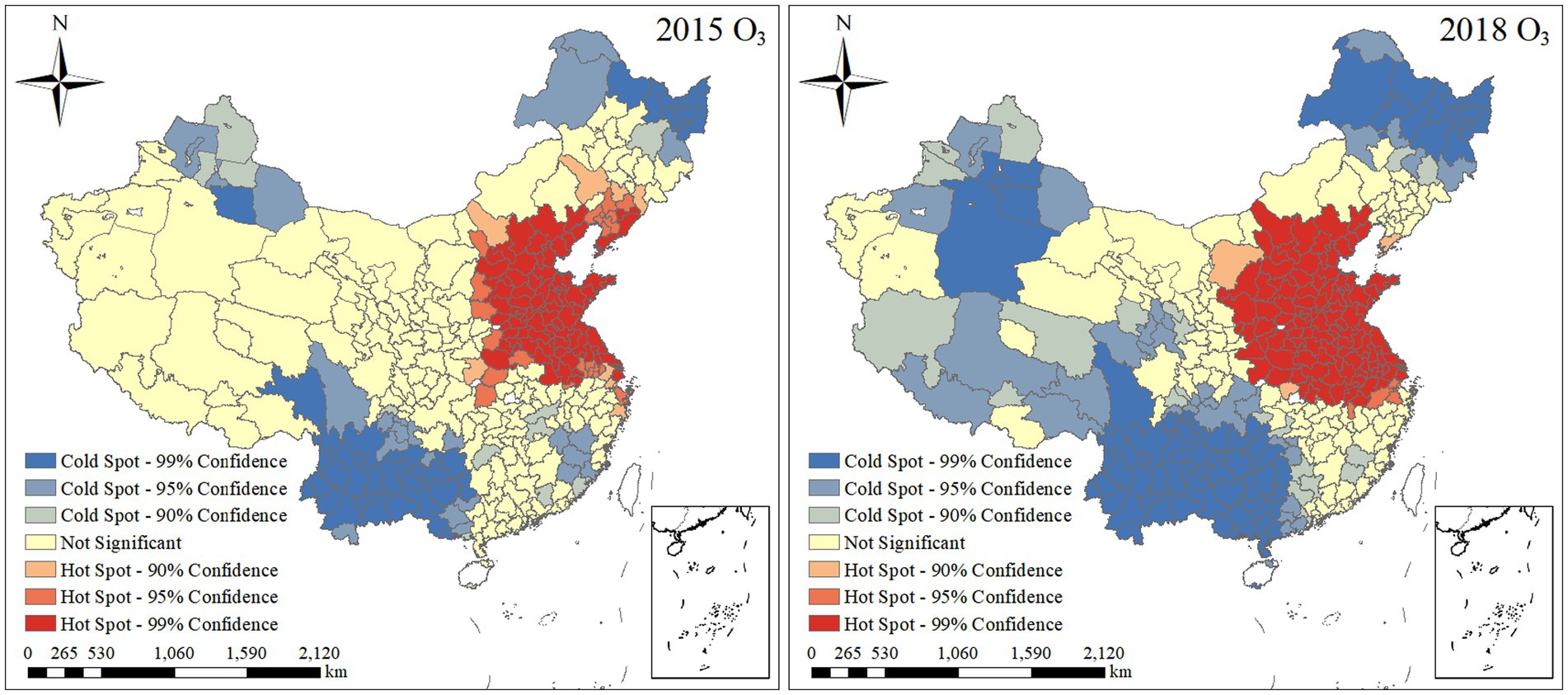
Figure 3. Annual spatial distribution of cold and hot spot of MDA8-90% across Chinese 337 cities in 2015 and 2018.

3.2.2. Seasonal spatial agglomeration characteristics

Spatial agglomeration characteristics of the O₃ concentration in spring, summer, fall, and winter in 2015 and 2018 are shown in Figure 4. In terms of season, in spring and summer, hot spots were mainly distributed in eastern, northern, and central provinces, including Inner Mongolia, Liaoning, Beijing, Hebei, Shanxi, Shandong, Henan, Anhui, Jiangsu, Shanghai, and Shaanxi. Therefore, the spring and summer were a critical period for O₃ pollution control in these provinces. Cold spots were mainly distributed in southwestern provinces, including Sichuan, Chongqing, Hunan, Jiangxi, Fujian, Yunnan, Guizhou, Guangxi, Guangdong, and Hainan. In fall, hot spots expanded in the southeast and were mainly concentrated in Hebei, Beijing, Shanxi, Shandong, Henan, Anhui, Jiangsu, Zhejiang, Jiangxi, Fujian, and Guangdong. Cold spots areas were gradually concentrated in the central provinces, including Sichuan, Chongqing, Guizhou, and Yunnan. Overall, O₃ pollution scale was large and these areas mainly concentrated in the central and eastern urban agglomerations, and showed distinct seasonal characteristics. Therefore, it is necessary to deeply strengthen the joint control measures between urban agglomerations in the central and eastern regions, and strengthen seasonal regulation, especially in spring and summer.

FIGURE 4

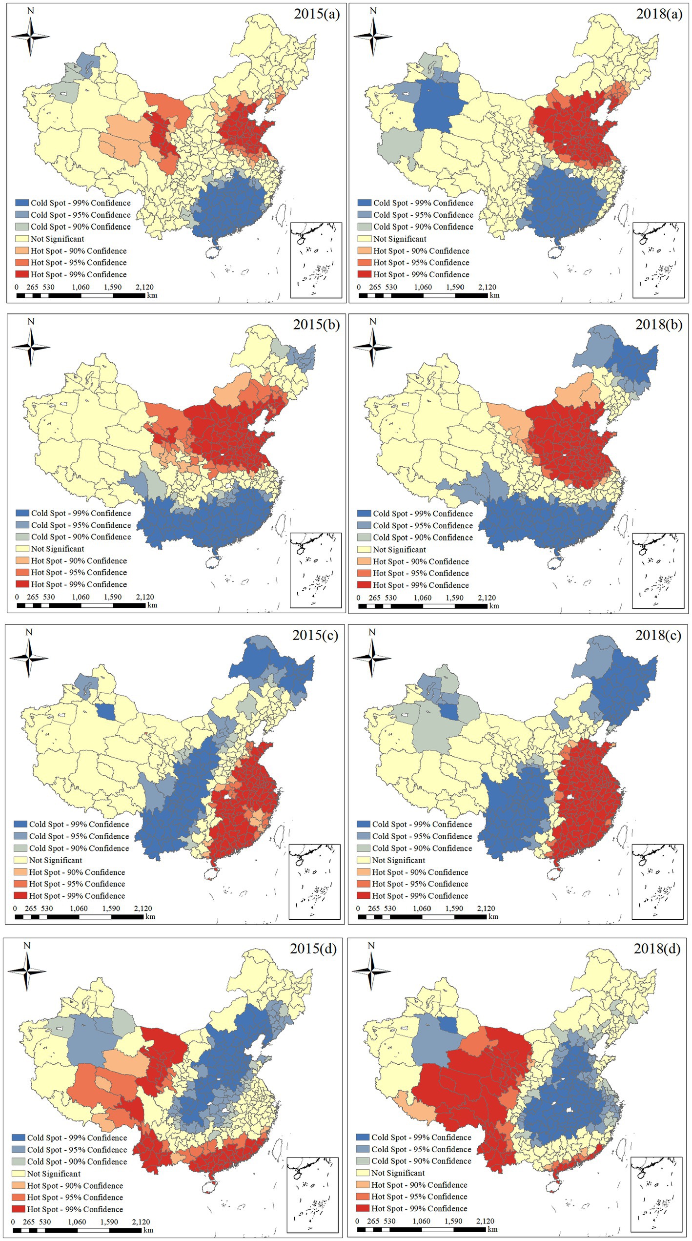
Figure 4. Seasonal evolution of MDA8 spatial agglomeration in 2015 and 2018: (A) spring, (B) summer, (C) fall, and (D) winter.

3.3. Population-weighted O₃ exposure risk

Only analysis of the spatiotemporal distributions of O₃ concentration cannot reflect the actual exposure risk of residents. To more scientifically reflect its potential residents’ exposure impact and screen the regions of particular concern, the population-weighted O₃ exposure risk evaluation was conducted based on formula (4) and shown in Figure 5. The population-weighted O₃ concentration values were calculated using a grid calculator, and a 1/2 standard deviation classification was used to divide the resulting population-weighted concentration values into eight levels. With the higher the rank, the higher the exposure risk of O₃. Low exposure risk was judged as level I and II, medium exposure risk was level III, IV, and V, and high exposure risk was level VI, VII, and VIII. It can be seen that the areas with high exposure risk of O₃ in 2015 and 2018 are quite similar and mainly concentrated in the central and eastern regions of China, such as Beijing, Tianjin, Hebei, Henan, and Anhui. In addition, the low exposure risk is mainly distributed in Tibet, Xinjiang, Qinghai, and other western regions.

FIGURE 5

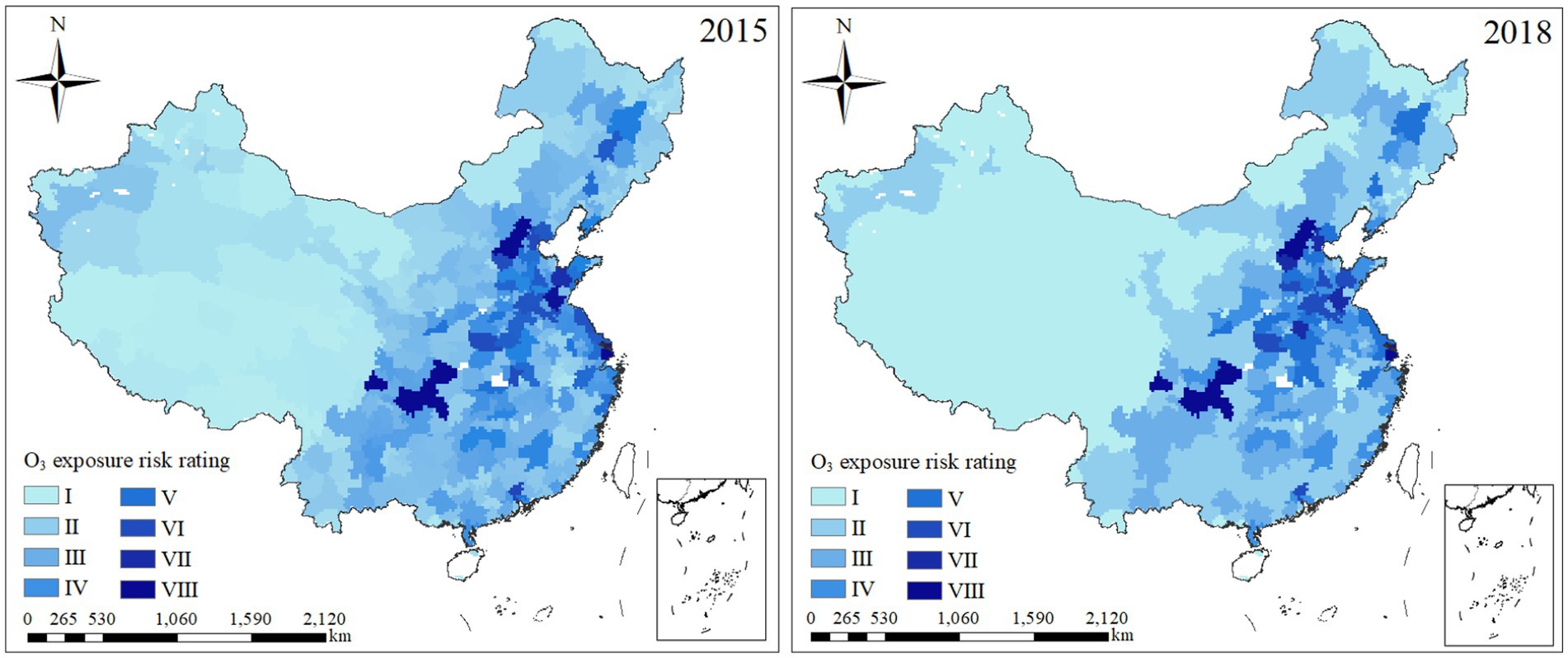
Figure 5. O₃ exposure risk rating under population-weighted conditions.

Considering the spatiotemporal distribution characteristics of O₃ and the population-weighted exposure risk. O₃ pollution has significant spatial aggregation characteristics, among them, O₃ concentration is more than 160 μg·m⁻³, exceedance rate more than 20% and high population-weighted exposure risk are mainly concentrated in the BTH-UA, CP-UA, and YRD-UA. To provide more accurate meteorological factors and socioeconomic driving factors analysis results in different regions, this study selected the 67 cities of BTH-UA, CP-UA, and YRD-UA as identified cities. Figure 6 shows location distribution of the BTH-UA, CP-UA, and YRD-UA in this study. The detailed list of 67 cities was shown in Supplementary Table S1.

FIGURE 6

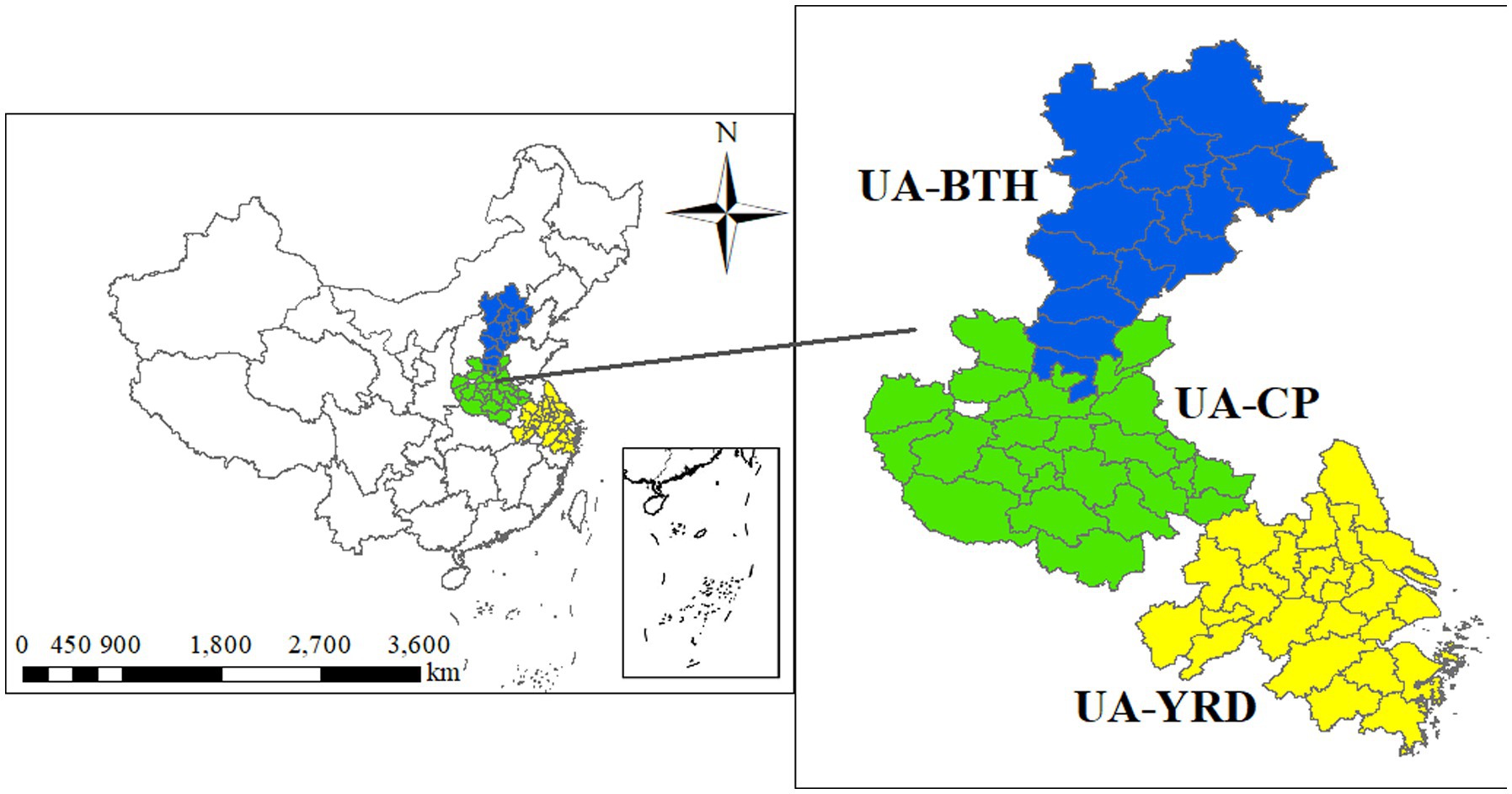
Figure 6. Location distribution of the BTH-UA, CP-UA, and YRD-UA.

3.4. Meteorological factor analysis

The concentration of O₃ was significantly affected by meteorological conditions. The main effects were divided into two aspects: first, meteorological conditions promoted the chemical conversion of precursors, such as NOx, CO, and VOCs, by affecting the photochemical reaction conditions of the O₃ (Huang et al., 2019), therefore, mading the O₃ concentration rise. Second, by affecting the local horizontal and vertical diffusion conditions (Blanchard and Fairley, 2001), and the O₃ concentration increase and decrease due to the volume fraction change.

3.4.1. Temperature

Table 2 shows that the correlation between O₃ concentration and temperature in different seasons. The annual O₃ concentration of the three urban agglomerations was significantly positively correlated with the temperature and the correlation is significant in the different seasons. In addition, seasonal differences were obvious. The correlation coefficient of the three urban agglomerations in spring and autumn was significantly higher than that in summer and winter. Among them, the CP-UA failed the confidence (bilateral) significance test of 0.01 in the winter in 2018 and the summer in 2015. One reason is possible that O₃ photochemical reaction is inefficient due to the influence of other factors, such as weak solar radiation in winter, rainfall and wind speed in summer (Chen X. P. et al., 2019).

TABLE 2

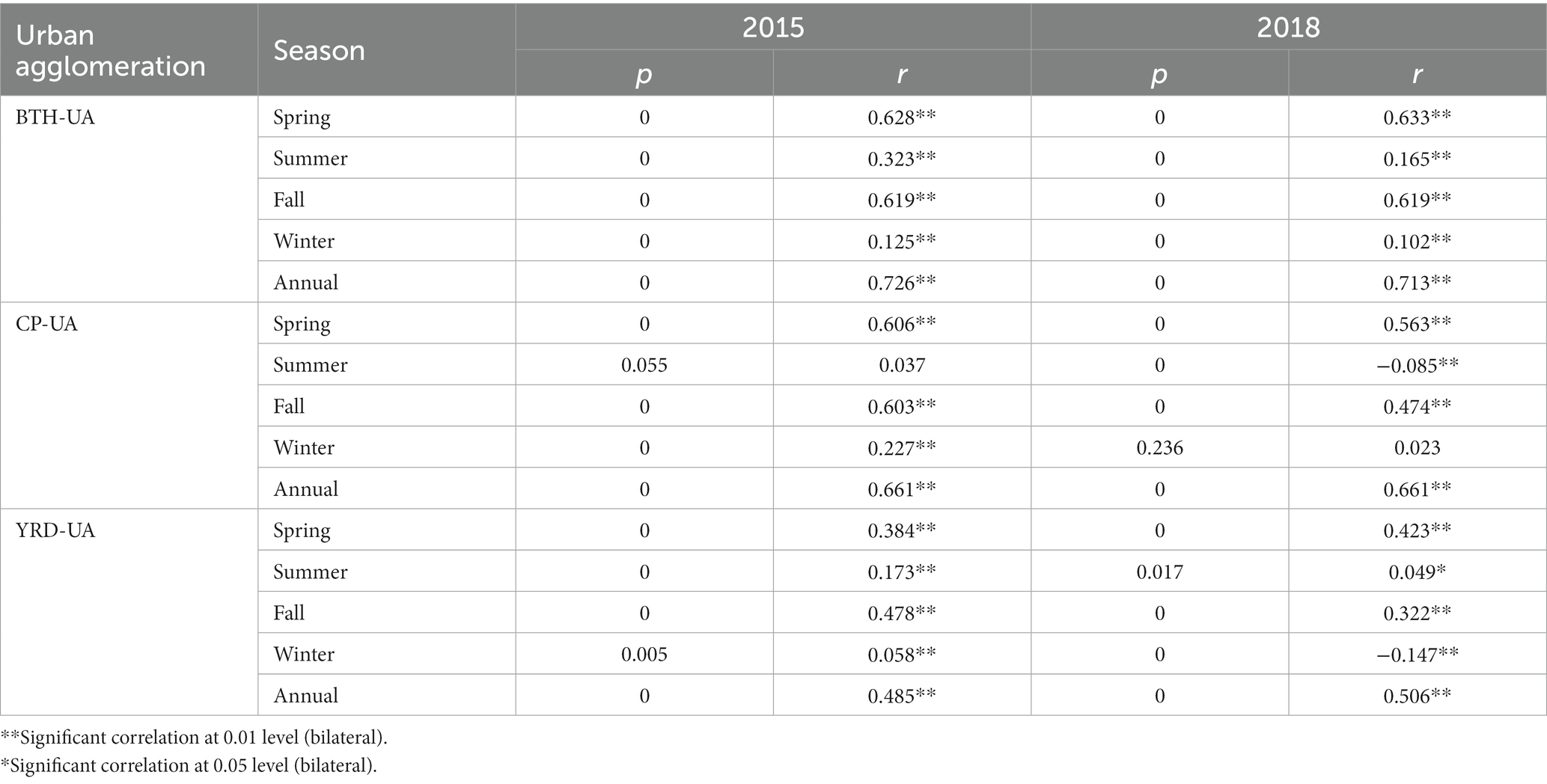
Table 2. Correlation between O₃ concentration and temperature in different seasons.

3.4.2. Relative humidity

Table 3 shows the correlation between O₃ concentration and relative humidity in different seasons. The annual relative humidity of the three urban agglomerations were significantly negatively correlated with O₃ concentration. In the three urban agglomerations, the absolute value of the correlation coefficient increased from north to south. The correlation was the most significant in summer, and the ranking of absolute value of correlation coefficient increased from north to south, which was the same as the annual ranking. It was due to that when the atmospheric relative humidity increases, it is accompanied by an increase in cloud cover, which leads to an increase in precipitation. These meteorological conditions are not conducive to the formation and accumulation of O₃, which leads to the decrease of O₃ concentration (Liang et al., 2019; Bai et al., 2022). In addition, it may be that when the RH is high, the photochemical decomposition of water vapor will produce more reactive groups and react with O₃, which reduces the concentration of O₃ (Tan et al., 2007). And this inhibition effect was more significant in the summer of the central and northern regions. Among them, the seasonal correlation coefficient of BTH-UA fluctuated significantly. The CP-UA was summer > spring and fall > winter, and the correlation coefficient was quite different, especially in summer and winter. The YRD-UA was summer > fall > spring > winter in 2015, and fall > spring > summer > winter in 2018, and the correlation coefficient fluctuation was small.

TABLE 3

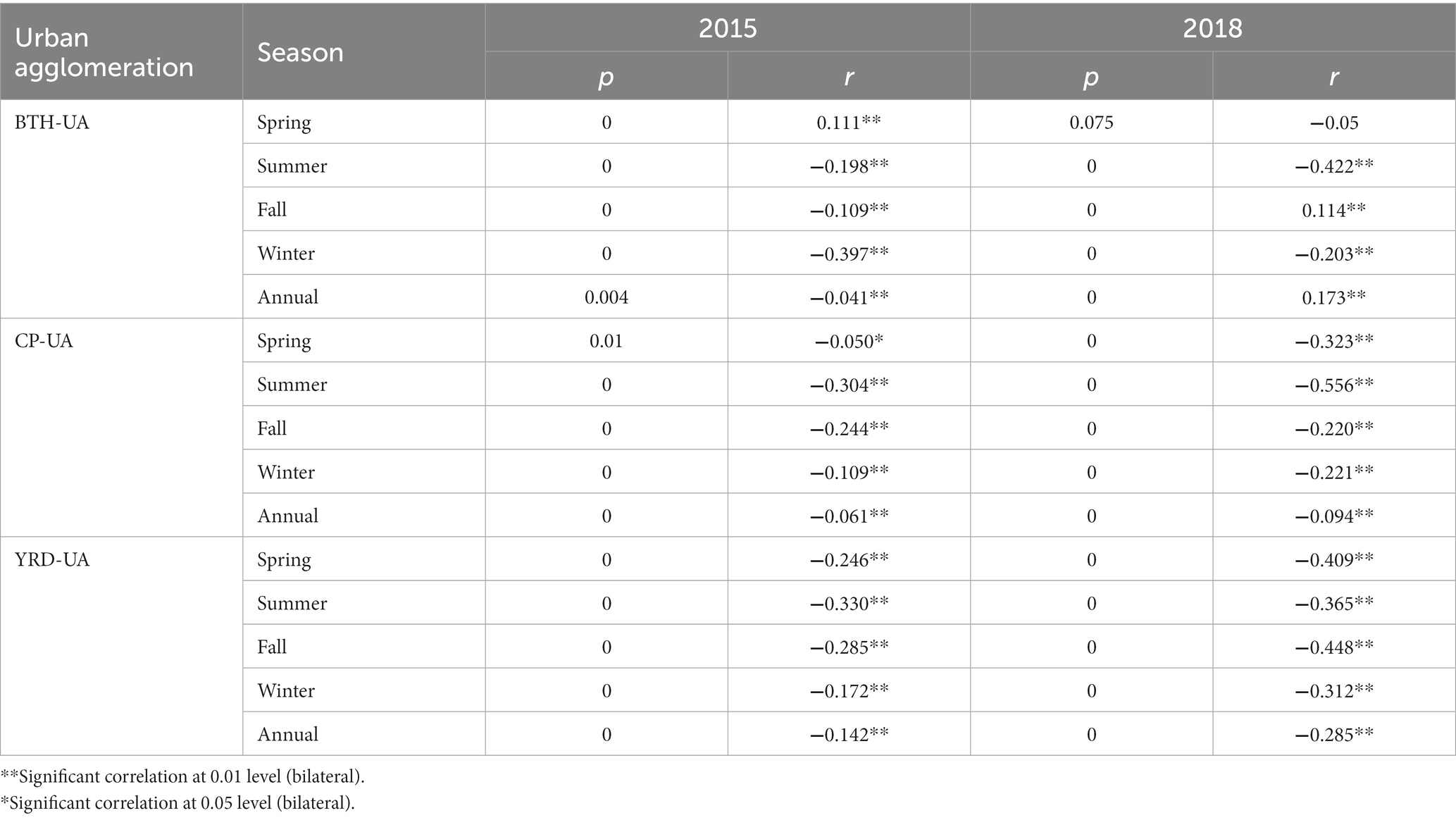
Table 3. Correlation between O₃ concentration and relative humidity in different seasons.

3.4.3. Wind speed

Wind speed, especially near-ground wind speed, determines the speed of pollutant handling and dilution (Yang et al., 2021). The correlation between O₃ concentration and wind speed in different seasons was shown in Table 4. The annual O₃ concentration of the CP-UA and the YRD-UA showed significantly negative correlation with the wind speed. While annual O₃ concentration of the BTH-UA was significantly positively correlated with the wind speed. From the seasonal point of view, the O₃ concentration in spring, summer, and autumn of the three urban agglomerations all showed significantly negative correlation with wind speed, while the O₃ concentration in winter showed significantly positive correlation with wind speed. It might have the reasons of O₃ increasing were the elevation of atmospheric boundary height and the increase of vertical momentum transport due to the increase of wind speed, which then promotes the transfer of O₃ to the ground (Chen et al., 2022; Liu et al., 2022). The reason for the O₃ decrease may be that the wind speed increases the horizontal diffusion movement of O₃.

TABLE 4

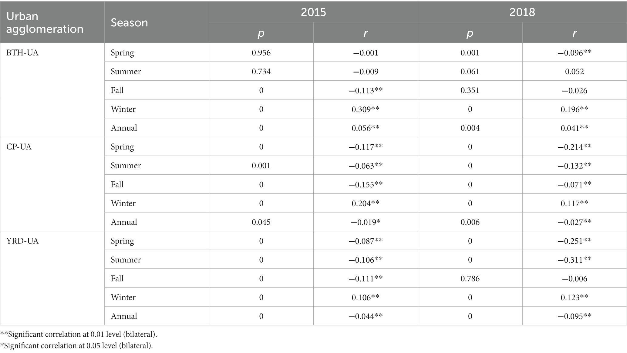
Table 4. Correlation between O₃ concentration and wind speed in different seasons.

The meteorological factors alter the O₃ concentration through physical and chemical processes. Among the meteorological factors, temperature was most associated with O₃ concentration in 2015 and 2018 (Tables 2–4). Temperature was directly affecting O₃ concentration by affecting the photochemical reaction generation efficiency of the O₃ (Chen et al., 2017), higher temperature, more frequent molecular collisions, and accelerated photochemical reaction rates. The wind speed and relative humidity had a negative effect on the O₃ concentration in BTH-UA, YRD-UA, and CP-UA. It was due to that high wind speed can promote horizontal diffusion and reduce the accumulation of air pollutants in headwind areas (Wang et al., 2019), indicating that the enhanced atmospheric diffusions efficiently reduced O₃ concentration levels. Moreover, O₃ pollution has changed significantly along with the season, so the seasonal O₃ pollution response measures should be strengthened. First, continue to strengthen the O₃ response in summer, and spring and fall should also be valued. Specifically, avoid or reduce VOCs process production in March–November, and stagger the peak emission in the O₃-prone period (12:00–17:00). Second, formulate a positive inventory of seasonal VOCs intensive emission reduction measures and implemented differentiated emission reduction measures. Enterprises that conform to the conditions of the positive inventory may not implement strengthened emission reduction. Third, in the critical areas such as BTH-UA, YRD-UA, and CP-UA, formulate pollution control plans for key industries, such as painting, printing, and textile, to help enterprises effectively carry out comprehensive control of VOCs.

3.5. Socioeconomic factors

3.5.1. Analysis of the VIF results

This study conducted multicollinearity tests of 14 socioeconomic factors of agglomeration regions in 2015 and 2018, including total population at year-end (TP), population density (PD), the gross domestic product (GDP), the per capita GDP (Per_GDP), share of the primary industry in GDP (%; Primary), share of the secondary industry in GDP (%; Secondary), share of the tertiary industry in the GDP (%; Tertiary), industrial soot emissions (ISE), annual average population (AP), total land area of administrative region (Administration), area of green land (Green), industrial SO₂ emission (ISO₂), average annual concentration of inhaled fine particulate matter (PM₁₀), and annual electricity consumption (AEC). The ArcGIS 10.2 analysis results were shown in Supplementary Table S2. The VIF of TP, GDP, Primary, Secondary, Tertiary, AP, and AEC were more than 10, which indicated that these seven factors had strong multicollinearity by themselves or with other factors, so these seven factors should be discarded. While PD, Per_GDP, ISE, Administration, Green, ISO₂, and PM₁₀ do not exist seriously multicollinearity, which can be used for GWR.

3.5.2. Analysis of the GWR results

The GWR model was fitted with seven socioeconomic factors (PD, Per_GDP, ISE, Administration, Green, ISO₂, and PM₁₀). The number of conditions on the sample points in 2015 and 2018 were all lower than 30, showing that there was no local collinearity. The coefficients of variables were all significant at the level of 1%, and the model estimation results were credible. The R² and adjusted R² were 0.46 and 0.31 in 2015, 0.66 and 0.56 in 2018 respectively, indicating the model had a better fit for both metrics in 2018. The standardized residual distribution was shown in Figure 7. The residue in the regression residue spatial distribution diagram was spatially random, demonstrating that the regression residue obeyed to the normal distribution. The regression results of normalized residual ranges were −2.51 to 2.07 in 2015, −3.11 to 1.63 in 2018, and values in the range of −2.00 to 2.00 accounted for 92.42 and 93.94% of the total results respectively, revealing the GWR model fit well. To further analyze the spatial changes of the various socioeconomic factors and the significance level of the O₃, Supplementary Table S3 reports the descriptive statistical results of the various socioeconomic factors of the GWR regression model.

FIGURE 7

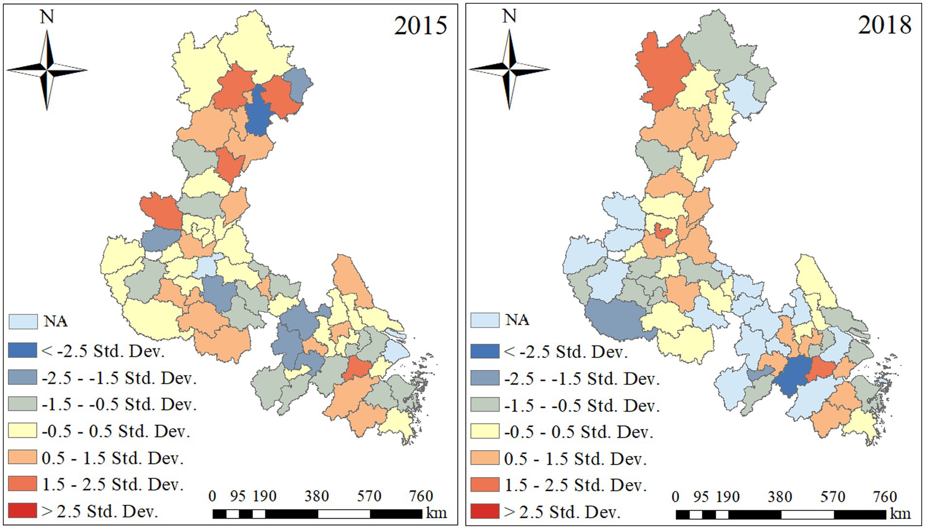
Figure 7. Standard residual error distribution of O₃ and socioeconomic factors.

The impact of PD, Per_GDP, ISE, Administration, Green, ISO₂, and PM₁₀ on O₃ pollution of urban agglomeration could be measured by the estimated coefficient of the influencing factors in various regions derived from the GWR model. The greater the coefficient of factor is, the greater the influence is, and the positive and negative of the coefficient represents the directionality of this factor. The parameter of the seven variables selected by the GWR differed in each region, indicating a spatial variation in the influence of each variable on the O₃ concentration.

3.5.3. The driving of urbanization factors

The urbanization factors included PD, Administration, and Green, and the adjusted R² were 0.42, 0.39, and 0.34 in 2015 respectively, and those were 0.57, 0.54, and 0.54 in 2018. This statistically demonstrated that the O₃ concentration distribution was closely related to the degree of urbanization. Figure 7 shows the distribution of the urbanization factors (PD, Administration, and Green) regression coefficient in 2015 and 2018.

Areas with high population density tend to have more pollution sources and pollution activity. Standardized residues for GWR between O₃ and PD ranged from −2.88 to 1.96 in 2015, and − 3.23 to 1.70 in 2018, values in the range of −2.00 to 2.00 accounted for 93.94 and 95.45% of the total results, respectively. Figure 7 shows that population density was positively associated with O₃ concentration in the majority cities, namely O₃ concentrations increased with the density of the population. The top five cities with the greatest correlation influence in 2015 were Chuzhou, Bengbu, Suzhou, Hefei, and Ma’anshan, located in the east of the CP-UA and the west of the YRD-UA. The top five cities with the highest correlation influence in 2018 were Qinhuangdao, Tangshan, Chengde, Xinyang, and Wuhu, mainly located in the BTH-UA. It was due to densely populated areas where human activity was more intense, and O₃ pollution was closely related to precursor emissions, such as VOCs, CO, and NOx. Therefore, the future control policies should be deeply concentrated in BTH-UA areas with high population density.

As shown in Figure 8, O₃ pollution was negatively correlated with Administration and Green in the majority of cities. Standardized residues for GWR between O₃ and Administration ranged from −2.85 to 2.12 in 2015, −3.72 to 2.32 in 2018, values in the range of −2.00 to 2.00 accounted for 92.42 and 92.42% of the total results, respectively. Standardized residues for GWR between O₃ and Green ranged from −3.05 to 1.70 in 2015, −2.84 to 1.74 in 2018, values in the range of −2.00 to 2.00 accounted for 93.94 and 95.45% of the total results, respectively. The high-value area was located in the YRD-UA, and the low-value area was located in the BTH-UA and the area between the border of the BTH-UA and CP-UA, which shows that the larger the green space area in this area is, the more it was conducive to reduce O₃ pollution. While some cities in the BTH-UA such as Tangshan, Qinhuangdao, Hengshui, Xingtai, Handan, and CP-UA such as Liaocheng, Puyang, Xinxiang, Zhengzhou, Administration, and Green were positively related to O₃ pollution in the majority cities. It was due to that the high O₃ concentration caused a certain degree of damage to plants, and greening did not play a role in reducing O₃ pollution. Overall, green space could help to improve air pollution and it was necessary to further expand green space in various cities.

FIGURE 8

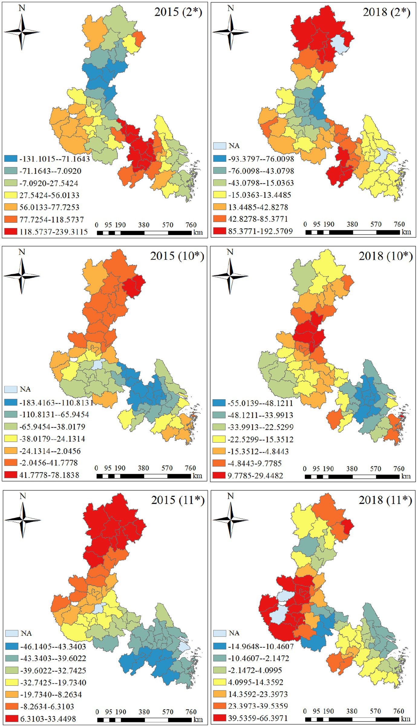
Figure 8. The distribution of the urbanization factors regression coefficient in 2015 and 2018. Population density (2^*), total land area of administrative region (10^*), and area of green land (11^*).

To alleviate O3 pollution caused by urbanization, the government needs to enhance the role of spatial allocation in urban planning, and create a spatial intensive urban pattern. Although central cities with high population density help to give full play to the advantages of agglomeration economy, high population will increase the ecological and environmental pressure and drive O₃ pollution. The reasonable layout and design of urban architectural could promote the dispersions of O₃ and improve the air quality. With the acceleration of urbanization in China, there were a large number of construction activities in developed and developing cities. Therefore, reasonable development plan of the administrative area and green space will be conducive to reduce O₃ pollution and improve the urban air quality.

3.5.4. The driving of economic structural factor

According to the analysis of GWR model, the adjusted R² of Per_GDP in 2015 and 2018 was 0.38 and 0.59, respectively (Supplementary Table S3). And as shown in Figure 9, O₃ pollution was positively correlated with Per_GDP in the majority cities. Standardized residues for GWR between O₃ and Per_GDP ranged from −2.76 to 1.66 in 2015, and − 2.83 to 1.71 in 2018, values in the range of −2.00 to 2.00 accounted for 93.94 and 95.45% of the total results, respectively. The high-value area was located in the YRD-UA, and the low-value area was located in the BTH-UA.

FIGURE 9

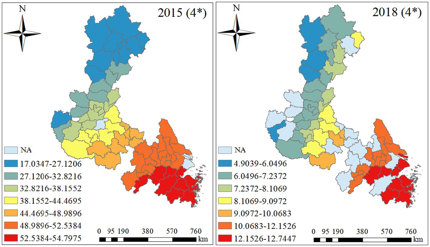
Figure 9. The distribution of the economic structural factor regression coefficient in 2015 and 2018. The per capita GDP (4^*).

Yang (2021) argued that China’s economic growth and environmental pollution showed a “U-shaped” relationship, that was, when the economic level was low, pollution improves with economic growth, and when it reaches an “inflection point,” pollution will deteriorate with economic growth. In this study, with the rapid development of economy from 2015 to 2018, O₃ pollution deteriorated. It could be seen that the BTH-UA, CP-UA, and YRD-UA were all in this “U-shaped” climbing period. With the further growth of the economy, regional O₃ pollution had a trend to deteriorate. Per_GDP was an important indicator reflecting the level of regional economic development. To realize the sustainable development of environmental protection and economic growth, the BTH-UA, CP-UA, and YRD-UA (especially YRD-UA) needed to build a joint pollution prevention and control model dominated by economic coordination and supplemented by policy and management coordination.

3.5.5. The driving of industrial production

In this study, the anthropogenic factors included ISE, ISO₂, and PM₁₀. The adjusted R² of ISE, ISO₂, and PM₁₀ were 0.34, 0.45, and 0.31 in 2015, and those were 0.56, 0.59, and 0.6 in 2018, respectively (Supplementary Table S3). Standardized residues for GWR between O₃ and ISE ranged from −3.25 to 1.73 and −2.81 to 1.57 in 2015, 2018, values in the range of −2.00 to 2.00 accounted for 95.45 and 93.94% of the total results, respectively. Standardized residues for GWR between O₃ and ISO₂ ranged from −2.80 to 1.79 in 2015, and − 2.83 to 1.78 in 2018, values in the range of −2.00 to 2.00 accounted for 93.94 and 96.97% of the total results, respectively. Standardized residues for GWR between O₃ and PM₁₀ ranged from −3.19 to 1.63, values in the range of −2.00 to 2.00 accounted for 93.94% in 2015, and ranged from −2.96 to 2.00 and values in the range of −2.00 to 2.00 accounted for 95.45% of the total results in 2018. O₃ pollution was positively correlated with the anthropogenic factors (ISE, ISO₂, and PM₁₀) in the majority cities as shown in Figure 10. It indicated that industrial soot emissions, industrial SO₂ emissions, and inhaled fine particulate matter increased O₃ pollution. The high-value area was located in the CP-UA and YRD-UA, and the low-value area was located in the BTH-UA.

FIGURE 10

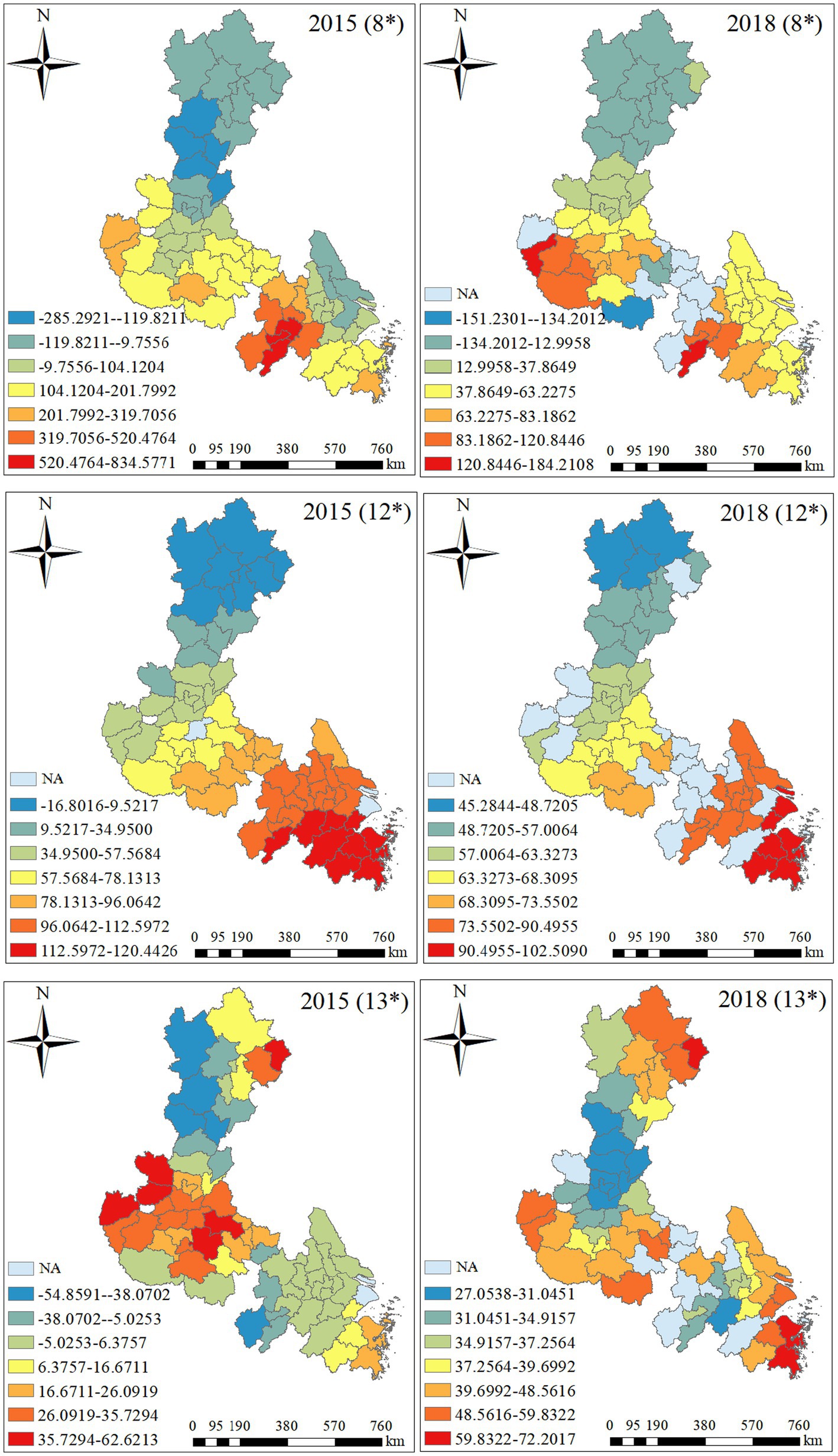
Figure 10. The distribution of the anthropogenic factors regression coefficient in 2015 and 2018. Industrial soot emissions (8^*), industrial SO₂ emissions (12^*), and average annual concentration of inhaled fine particulate matter (13^*).

Compared with 2015, the impacts of ISE on O₃ pollution in 2018 were reduced, while the impacts of ISO₂ and PM₁₀ emission were more significant. These mean that the upcoming industrial emission control policy should place greater emphasis on limiting the SO₂ and PM₁₀ emissions in the CP-UA and YRD-UA. Specifically, SO₂ emissions should be strictly controlled in the YRD-UA. And to control PM₁₀ emissions, all kinds of open-air incineration should be strictly controlled and the government should strengthen the main responsibility of CP-UA governments for straw burning at all levels. In addition, the major sources of pollution in SO₂, soot, and PM₁₀ were industrial emissions. Therefore, the government needs to grasp the development direction of environmental protection technology of the “Made in China 2025” strategy, and encourage industrial enterprises to research, develop and introduce environmental protection technology, and accelerate the adjustment and optimization of the industrial structure in the BTH-UA, CP-UA, and YRD-UA. It will help to reduce the environmental burden. Specifically, control of exhaust pollution from mobile pollution sources should be strengthened and rigid industrial emission standards should be established, factories, which could not meet the standards, should be thus eliminated.

4. Conclusion

Spatiotemporal variation of urban surface O₃ and population-weighted exposure risk characteristics were analyzed across China and the three typical urban agglomerations (BTH-UA, YRD-UA, and CP-UA) were identified as the hot regions, where their O₃ concentration exceed 160 μg·m⁻³, exceedance rate more than 20% and relatively high population-weighted exposure risk. The correlation analysis results in the hot regions show that high surface temperature, low relative humidity, and low wind speed were positive to O₃ increase and O₃ pollution has changed significantly along with the season. So continue to strengthen the O₃ response in summer and formulate a positive inventory of seasonal VOCs intensive emission reduction measures and implemented differentiated emission reduction measures. Moreover, GWR results revealed that O₃ in majority cities were positively related with PD, Per_GDP, ISE, ISO₂, and PM₁₀, while negatively related with Administration and Green. Then, the urban agglomerations management strategies were established: (i) reasonable development plan of the administrative area and green space will be conducive to reduce O₃ pollution and improve the urban air quality; (ii) the BTH-UA, CP-UA, and YRD-UA (especially YRD-UA) needed to build a joint pollution prevention and control model dominated by economic coordination and supplemented by policy and management coordination; and (iii) the upcoming industrial emission control policy should place greater emphasis on limiting the SO₂ and PM₁₀ emissions in the CP-UA and YRD-UA. And control of exhaust pollution from mobile pollution sources should be strengthened and rigid industrial emission standards should be established, factories, which could not meet the standards, should be thus eliminated.

Data availability statement

The raw data supporting the conclusions of this article will be made available by the authors, without undue reservation.

Author contributions

SK: writing—original draft preparation and data analysis. TW and FL: methodology, reviewing and revision, and validation. JY: investigation and reviewing. ZQ: coordinate organization and reviewing. All authors contributed to the article and approved the submitted version.

Funding

This study was supported by National Social Science Foundation of China (Youth Fund: 19CGL042), Hubei Provincial Outstanding Young Science and Technology Innovation Team Project (T2021032) and the Fundamental Research Funds for the Central Universities, Zhongnan University of Economics and Law (2722023EZ009, 202351418).

Conflict of interest

The authors declare that the research was conducted in the absence of any commercial or financial relationships that could be construed as a potential conflict of interest.

Publisher’s note

All claims expressed in this article are solely those of the authors and do not necessarily represent those of their affiliated organizations, or those of the publisher, the editors and the reviewers. Any product that may be evaluated in this article, or claim that may be made by its manufacturer, is not guaranteed or endorsed by the publisher.

Supplementary material

The Supplementary material for this article can be found online at: https://www.frontiersin.org/articles/10.3389/fevo.2023.1103503/full#supplementary-material

References

Anselin, L. (2010). Local indicators of spatial association-LISA. Geogr. Anal. 27, 93–115. doi: 10.1111/j.1538-4632.1995.tb00338.x

CrossRef Full Text | Google Scholar

Bai, L. Y., Feng, J. Z., Li, Z. W., Han, C. M., Yan, F. L., and Ding, Y. X. (2022). Spatiotemporal dynamics of surface ozone and its relationship with meteorological factors over the Beijing-Tianjin-Tangshan region, China, from 2016 to 2019. Sensors 22:4854. doi: 10.3390/s22134854

PubMed Abstract | CrossRef Full Text | Google Scholar

Blanchard, C. L., and Fairley, D. (2001). Spatial mapping of VOC and NOx-limitation of ozone formation in Central California. Atmos. Environ. 35, 3861–3873. doi: 10.1016/S1352-2310(01)00153-4

CrossRef Full Text | Google Scholar

Chang, L. Y., He, F. F., Tie, X. X., Xu, J. M., and Gao, W. (2021). Meteorology driving the highest ozone level occurred during mid-spring to early summer in Shanghai. Sci. Total Environ. 785:147253. doi: 10.1016/j.scitotenv.2021.147253

CrossRef Full Text | Google Scholar

Che, H. Z., Gui, K., Xia, X. G., Wang, Y. Q., Holben, B., Goloub, P., et al. (2019). Large contribution of meteorological factors to inter-decadal changes in regional aerosol optical depth. Atmos. Chem. Phys. Discuss. 19, 10497–10523. doi: 10.5194/acp-19-10497-2019

CrossRef Full Text | Google Scholar

Chen, Y. G. (2021). An analytical process of spatial autocorrelation functions based on Moran's index. PLoS One 16:e0249589. doi: 10.1371/journal.pone.0249589

PubMed Abstract | CrossRef Full Text | Google Scholar

Chen, X. P., Ju, T. Z., Zhang, J. Y., Xian, L., Wang, P. Y., and Zhang, S. C. (2019). Correlation between atmospheric ozone and precursor and meteorological factors in Lanzhou city. Res. Environ. Sci. 32, 2075–2083. doi: 10.13198/j.issn.1001-6929.2019.06.01

CrossRef Full Text | Google Scholar

Chen, X. Y., Li, F., Zhang, J. D., Zhou, W., Wang, X. Y., and Fu, H. J. (2020). Spatiotemporal mapping and multiple driving forces identifying of PM_2.5 variation and its joint management strategies across China. J. Clean. Prod. 250:119534. doi: 10.1016/j.jclepro.2019.119534

CrossRef Full Text | Google Scholar

Chen, B., Yang, X. B., and Xu, J. J. (2022). Spatio-temporal variation and influencing factors of ozone pollution in Beijing. Atmosfera 13:359. doi: 10.3390/atmos13020359

CrossRef Full Text | Google Scholar

Chen, Y., Zhang, J. P., and Huang, Z. Z. (2017). Spatial-temporal variation of surface ozone in Guangzhou and its relations with meteorological factors. Environ. Monitor. China. 33, 99–10. doi: 10.19316/j.issn.1002-6002.2017.04.13

CrossRef Full Text | Google Scholar

Chen, Z. Y., Zhuang, Y., Xie, X. M., Chen, D. L., Cheng, N. L., Yang, L., et al. (2019). Understanding long-term variations of meteorological influences on ground ozone concentrations in Beijing during 2006-2016. Environ. Pollut. 245, 29–37. doi: 10.1016/j.envpol.2018.10.117

PubMed Abstract | CrossRef Full Text | Google Scholar

Cheng, N. L., Chen, Z. Y., Sun, F., Sun, R. W., Dong, X., Xie, X. M., et al. (2018). Ground ozone concentrations over Beijing from 2004 to 2015: variation patterns, indicative precursors and effects of emission-reduction. Environ. Pollut. 237, 262–274. doi: 10.1016/j.envpol.2018.02.051

PubMed Abstract | CrossRef Full Text | Google Scholar

Dong, H., Cheng, L., Wang, H. Y., Zhao, X. H., and Zhu, Y. (2021). Analysis of ozone pollution characteristics and meteorological factors in Anhui province. Environ. Monitor. China. 37, 58–68. doi: 10.19316/j.issn.1002-6002.2021.01.09

CrossRef Full Text | Google Scholar

Environmental Protection Department (EPD) (2012). GB3095-2012 Ambient Air Quality Standards. Beijing: China Environ. Sci. Publish. House

Google Scholar

Fu, Q. Y., and Kan, H. D. (2004). Methods for health risk assessment of urban air pollution, unit 4: air pollution exposure assessment, section 2: dispersion model and population-weighted air pollution exposure assessment. J. Environ. Health 21, 414–416. doi: 10.3969/j.issn.1001-5914.2004.06.024

CrossRef Full Text | Google Scholar

Guo, J. P., Deng, M. J., Lee, S. S., Wang, F., Li, Z. Q., Zhai, P. M., et al. (2016). Delaying precipitation and lightning by air pollution over the Pearl River Delta. Part I: observational analyses. J. Geophys. Res. Atmos. 121, 6472–6488. doi: 10.1002/2015JD023257

CrossRef Full Text | Google Scholar

Harmens, H., Hayes, F., Mills, G., Sharps, K., Osborne, S., and Pleijel, H. (2018). Wheat yield responses to stomatal uptake of ozone: peak vs rising background ozone conditions. Atmos. Environ. 173, 1–5. doi: 10.1016/j.atmosenv.2017.10.059

CrossRef Full Text | Google Scholar

He, J. J., Gong, S. L., Yu, Y., Yu, L. J., Wu, L., Mao, H. J., et al. (2017). Air pollution characteristics and their relation to meteorological conditions during 2014-2015 in major Chinese cities. Environ. Pollut. 223, 484–496. doi: 10.1016/j.envpol.2017.01.050

PubMed Abstract | CrossRef Full Text | Google Scholar

He, Y. P., Wang, H. L., Wang, H. C., Xu, X. Q., Li, Y. M., and Fan, S. J. (2021). Meteorology and topographic influences on nocturnal ozone increase during the summertime over Shaoguan. Chin. Atmos. Environ. 256:118459. doi: 10.1016/j.atmosenv.2021.118459

CrossRef Full Text | Google Scholar

Hu, C. Y., Kang, P., Jaffe, D. A., Li, C. K., Zhang, X. L., Wu, K., et al. (2021). Understanding the impact of meteorology on ozone in 334 cities of China. Atoms. Environ. 248:118221. doi: 10.1016/j.atmosenv.2021.118221

CrossRef Full Text | Google Scholar

Huang, X. G., Shao, T. J., Zhao, J. B., Cao, J. J., and Yue, D. P. (2019). Impact of meteorological factors and precursors on spatial distribution of ozone concentration in eastern China. China Environ. Sci. 36, 2273–2282. doi: 10.19674/j.cnki.issn1000-6923.2019.0270

CrossRef Full Text | Google Scholar

Karlsson, P. E., Klingberg, J., Engardt, M., Andersson, C., Langner, J., Karlsson, G. P., et al. (2017). Past, present and future concentrations of ground-level ozone and potential impacts on ecosystems and human health in northern Europe. Sci. Total Environ. 576, 22–35. doi: 10.1016/j.scitotenv.2016.10.061

PubMed Abstract | CrossRef Full Text | Google Scholar

Li, P., De Marco, A., Feng, Z. Z., Anav, A., Zhou, D. J., and Paoletti, E. (2018). Nationwide ground-level ozone measurements in China suggest serious risks to forests. Environ. Pollut. 237, 803–813. doi: 10.1016/j.envpol.2017.11.002

PubMed Abstract | CrossRef Full Text | Google Scholar

Liang, Y., Huang, D., Li, J. Q., Song, M. H., Zhong, K. Y., and Cheng, X. (2020). Study on the influence of meteorological factors on the ozone concentration in Panzhihua city. J. Green Sci. Technol. 12, 98–104. doi: 10.16663/j.cnki.lskj.2020.12.033

CrossRef Full Text | Google Scholar

Liang, J. N., Ma, Q. X., Wang, P., and Liu, J. (2019). Analysis of the relationship between ozone and meteorological factors in summer at airport new city of xi Xian new area, China. Ecol. Environ. Sci. 28, 2020–2026. doi: 10.16258/j.cnki.1674-5906.2019.10.012

CrossRef Full Text | Google Scholar

Liu, C., Dong, J. L., Tian, L., and Kong, H. J. (2022). Analysis of ozone concentration characteristics and meteorological factors in Zhengzhou in 2017[J]. Meteorol. Environ. Sci. 45, 33–38. doi: 10.16765/j.cnki.1673-7148.2022.04.004

CrossRef Full Text | Google Scholar

Liu, H., Liu, S., Xue, B. R., Lv, Z. F., Meng, Z. H., Yang, X. F., et al. (2018). Ground-level ozone pollution and its health impacts in China. Atmos. Environ. 173, 223–230. doi: 10.1016/j.atmosenv.2017.11.014

CrossRef Full Text | Google Scholar

Liu, P. F., Song, H. Q., Wang, T. H., Wang, F., Li, X. Y., Miao, C. H., et al. (2020). Effects of meteorological conditions and anthropogenic precursors on ground-level ozone concentrations in Chinese cities. Environ. Pollut. 262:114366. doi: 10.1016/j.envpol.2020.114366

PubMed Abstract | CrossRef Full Text | Google Scholar

Liu, H. L., Zhang, M. G., and Han, X. (2020). A review of surface ozone source apportionment in China. Atmos. Ocean. Sci. Lett. 13, 470–484. doi: 10.1080/16742834.2020.1768025

CrossRef Full Text | Google Scholar

Ministry of Ecology and Environment of the People’s Republic of China (MEE-PRC) (2016). 2015 China Ecological and Environment Bulletin. Beijing: China Environmental Publishing Group

Google Scholar

Qu, L. L., Liu, S. J., Ma, L. L., Zhang, Z. Z., Du, J. H., Zhou, Y. H., et al. (2020). Evaluating the meteorological normalized PM2.5 trend (2014-2019) in the “2+26” region of China using an ensemble learning technique. Environ. Pollut. 266:115346. doi: 10.1016/j.envpol.2020.115346

PubMed Abstract | CrossRef Full Text | Google Scholar

Tan, J. G., Lu, G. L., Geng, F. H., and Zhen, X. R. (2007). Analysis and prediction of surface O₃ concentration and related meteorological factors in summer time in urban area of Shanghai. J. Trop. Meteorol. 23, 515–520. doi: 10.16032/j.issn.1004-4965.2007.05.014

CrossRef Full Text | Google Scholar

Wang, Y. C., Chen, J., Wang, Q. Y., Qin, Q. D., Ye, J. H., Han, Y. M., et al. (2019). Increased secondary aerosol contribution and possible processing on polluted winter days in China. Environ. Int. 127, 78–84. doi: 10.1016/j.envint.2019.03.021

PubMed Abstract | CrossRef Full Text | Google Scholar

Wang, S. J., Gao, S., and Chen, J. (2020). Spatial heterogeneity of driving factors of urban haze pollution in China based on GWR model. Geogr. Res. 39, 651–668. doi: 10.11821/dlyj020181389

CrossRef Full Text | Google Scholar

Wang, Z. B., Li, J. X., and Liang, L. W. (2020). Spatio-temporal evolution of ozone pollution and its influencing factors in the Beijing-Tianjin-Hebei urban agglomeration. Environ. Pollut. 256:113419. doi: 10.1016/j.envpol.2019.113419

PubMed Abstract | CrossRef Full Text | Google Scholar

Wang, Y. C., Liu, C. G., Wang, Q. Y., Qin, Q. D., Ren, H. H., and Cao, J. J. (2021). Impacts of natural and socioeconomic factors on PM2.5 from 2014 to 2017. J. Environ. Manag. 284:112071. doi: 10.1016/j.jenvman.2021.112071

PubMed Abstract | CrossRef Full Text | Google Scholar

Wang, X. L., Zhao, W. J., Li, L. J., Yang, X. C., Jiang, J. F., and Sun, S. (2020). Characteristics of spatiotemporal distribution of O₃ in China and impact analysis of socio-economic factors. Earth Environ. 48, 66–75. doi: 10.14050/j.cnki.1672-9250.2020.48.006

CrossRef Full Text | Google Scholar

Wei, P. R., Shao, T. J., Huang, X. G., and Zhang, Z. D. (2020). Study of spatio-temporal variation and the influencing factors of ozone in Northeast China during 2015-2018. J. Ecol. Rural Environ. 36, 988–997. doi: 10.19741/j.issn.1673-4831.2019.0741

CrossRef Full Text | Google Scholar

Yan, G., Xue, W. B., Lei, Y., Ning, M., Wu, W. L., and Liu, W. (2020). Situation and control measures of ozone pollution in China. Environ. Prot. 48, 15–19. doi: 10.14026/j.cnki.0253-9705.2020.15.003

CrossRef Full Text | Google Scholar

Yang, C. S. (2021). Relationship between environmental pollution and economic growth-an empirical analysis based on China’s environmental Kuznets curve. J. Ankang Univ. 33, 112–121. doi: 10.16858/j.issn.1674-0092.2021.02.019

CrossRef Full Text | Google Scholar

Yang, Y. L., Hao, J. F., and Zhao, Y. G. (2021). Characteristics of ozone pollution and influence of meteorological factors in typical city in central and southern Hebei Province. Environ. Sci. Manag. 46, 5–9. doi: 10.3969/j.issn.1673-1212.2021.05.005

CrossRef Full Text | Google Scholar

Zhan, C. C., Xie, M., Liu, J., Wang, T. J., Xu, M., Chen, B., et al. (2021). Surface ozone in the Yangtze River Delta, China: a synthesis of basic features, meteorological driving factors, and health impacts. Atmosfera 126:e2020JD033600. doi: 10.1029/2020JD033600

CrossRef Full Text | Google Scholar

Zhao, W., Fan, S. J., Guo, H., Gao, B., Sun, J. R., and Chen, L. G. (2016). Assessing the impact of local meteorological variables on surface ozone in Hong Kong during 2000-2015 using quantile and multiple line regression models. Atmos. Environ. 144, 182–193. doi: 10.1016/j.atmosenv.2016.08.077

CrossRef Full Text | Google Scholar

Zhao, S. P., Yin, D. Y., Yu, Y., Kang, S. C., Qin, D. H., and Dong, L. X. (2020). PM_2.5 and O₃ pollution during 2015-2019 over 367 Chinese cities: spatiotemporal variations, meteorological and topographical impacts. Environ. Pollut. 264:114694. doi: 10.1016/j.envpol.2020.114694

PubMed Abstract | CrossRef Full Text | Google Scholar

Zhou, M. W., Kang, P., Wang, K. K., Zhang, X. L., and Hu, C. Y. (2020). The spatio-temporal aggregation pattern of ozone concentration in China from 2016 to 2018. China. Environ. Sci. 40, 1963–1974. doi: 10.19674/j.cnki.issn1000-6923.2020.0222

CrossRef Full Text | Google Scholar

Zhou, X. S., Liao, Z. H., Wang, M., Chen, J. L., Dong, J., Zhao, X. F., et al. (2019). Characteristics of ozone concentration and its relationship with meteorological factors in Zhuhai during 2013-2016. Acta Sci. Circum. 39, 143–153. doi: 10.13671/j.hjkxxb.2018.0390

CrossRef Full Text | Google Scholar

Ziemke, J. R., Oman, L. D., Strode, S. A., Douglass, A. R., Olsen, M. A., McPeters, R. D., et al. (2019). Trends in global tropospheric ozone inferred from a composite record of TOMS/OMI/MLS/OMPS satellite measurements and the MERRA-2 GMI simulation. Atmos. Chem. Phys. 19, 3257–3269. doi: 10.5194/acp-19-3257-2019

CrossRef Full Text | Google Scholar