 Dena J. Clink
 Isabel Kier
 Abdul Hamid Ahmad2
 Holger Klinck
- 1K. Lisa Yang Center for Conservation Bioacoustics, Cornell Lab of Ornithology, Cornell University, Ithaca, NY, United States
- 2Institute for Tropical Biology and Conservation, Universiti Malaysia Sabah, Kota Kinabalu, Sabah, Malaysia
Passive acoustic monitoring (PAM) allows for the study of vocal animals on temporal and spatial scales difficult to achieve using only human observers. Recent improvements in recording technology, data storage, and battery capacity have led to increased use of PAM. One of the main obstacles in implementing wide-scale PAM programs is the lack of open-source programs that efficiently process terabytes of sound recordings and do not require large amounts of training data. Here we describe a workflow for detecting, classifying, and visualizing female Northern grey gibbon calls in Sabah, Malaysia. Our approach detects sound events using band-limited energy summation and does binary classification of these events (gibbon female or not) using machine learning algorithms (support vector machine and random forest). We then applied an unsupervised approach (affinity propagation clustering) to see if we could further differentiate between true and false positives or the number of gibbon females in our dataset. We used this workflow to address three questions: (1) does this automated approach provide reliable estimates of temporal patterns of gibbon calling activity; (2) can unsupervised approaches be applied as a post-processing step to improve the performance of the system; and (3) can unsupervised approaches be used to estimate how many female individuals (or clusters) there are in our study area? We found that performance plateaued with >160 clips of training data for each of our two classes. Using optimized settings, our automated approach achieved a satisfactory performance (F1 score ~ 80%). The unsupervised approach did not effectively differentiate between true and false positives or return clusters that appear to correspond to the number of females in our study area. Our results indicate that more work needs to be done before unsupervised approaches can be reliably used to estimate the number of individual animals occupying an area from PAM data. Future work applying these methods across sites and different gibbon species and comparisons to deep learning approaches will be crucial for future gibbon conservation initiatives across Southeast Asia.
Introduction
Passive acoustic monitoring
Researchers worldwide are increasingly interested in passive acoustic monitoring (PAM), which relies on autonomous recording units to monitor vocal animals and their habitats. Increased availability of low-cost recording units (Hill et al., 2018; Sethi et al., 2018; Sugai et al., 2019), along with advances in data storage capabilities, makes the use of PAM an attractive option for monitoring vocal species in inaccessible areas where the animals are difficult to monitor visually (such as dense rainforests) or when the animals exhibit cryptic behavior (Deichmann et al., 2018). Even in cases where other methods such as visual surveys are feasible, PAM may be superior as it may be able to detect animals continuously for extended periods of time, at a greater range than visual methods, can operate under any light conditions, and is more amenable to automated data collection than visual or trapping techniques (Marques et al., 2013). In addition, PAM provides an objective, non-invasive method that limits observer bias in detection of target signals.
One of the most widely recognized benefits of using acoustic monitoring, apart from the potential to reduce the amount of time needed for human observers, is that there is a permanent record of the monitored soundscape (Zwart et al., 2014; Sugai and Llusia, 2019). In addition, the use of archived acoustic data allows for multiple analysts at different times to review and validate detections/classifications, as opposed to point-counts where one or multiple observers, often with varying degrees of experience, collect the data in-situ. It is, therefore, not surprising that, in many cases, analysis of recordings taken by autonomous recorders can be more effective than using trained human observers in the field. For example, a comparison of PAM and human observers to detect European nightjars (Caprimulgus europaeus) showed that PAM detected nightjars during 19 of 22 survey periods, while surveyors detected nightjars on only six of these occasions (Zwart et al., 2014). An analysis of 21 bird studies that compared detections by human observers and detections from acoustic data collected using autonomous recorders found that for 15 of the studies, manual analysis of PAM acoustic data led to results that were equal to or better than results from point counts done using human observers (Shonfield and Bayne, 2017). Despite the rapidly expanding advances in PAM technology, the use of PAM is limited by a lack of widely applicable analytical methods and the limited availability of open-source audio processing tools, particularly for the tropics, where soundscapes are very complex (Gibb et al., 2018).
Interest in the use of PAM to monitor nonhuman primates has increased in recent years, with one of the foundational papers using PAM to estimate occupancy of three signal types: chimpanzee buttress drumming (Pan troglodytes) and the loud calls of the Diana monkey (Cercopithecus diana) and king colobus monkey (Colobus polykomos) in Taï National Park, Côte d’Ivoire (Kalan et al., 2015). The authors found that occurrence data from PAM combined with automated processing methods was comparable to that collected by human observers. Since then, PAM has been used to investigate chimpanzee group ranging and territory use (Kalan et al., 2016), vocal calling patterns of gibbons (Hylobates funereus; Clink et al., 2020b) and howler monkeys (Alouatta caraya; Pérez-Granados and Schuchmann, 2021), occupancy modeling of gibbons (Nomascus gabriellae; Vu and Tran, 2019) and density estimation of pale fork-marked lemurs (Phaner pallescens) based on calling bout rates (Markolf et al., 2022).
Acoustic analysis of long-term datasets
Traditional approaches for finding signals of interest include hand-browsing spectrograms to identify signals of interest using programs such as Raven Pro (K. Lisa Yang Center for Conservation Bioacoustics, Ithaca, NY, USA). This approach can reduce processing time relative to listening to the recordings but requires trained analysts and substantial human investment. Another approach is hand-browsing of long-term spectral averages (LTSAs), which still requires a significant time investment, but allows analysts to process data at a faster rate than hand-browsing of regular spectrograms, as LTSAs provide a visual representation of the soundscape over a larger time period [days to weeks to years (Wiggins, 2003; Clink et al., 2020b)]. However, particularly with the advances in data storage capabilities and deployment of arrays of recorders collecting data continuously, the amount of time necessary for hand-browsing or listening to recordings for signals of interest is prohibitive and is not consistent with conservation goals that require rapid assessment. This necessitates reliable, automated approaches to efficiently process large amounts of acoustic data.
Automated detection and classification
Machine listening, a fast-growing field in computer science, is a form of artificial intelligence that “learns” from training data to perform particular tasks, such as detecting and classifying acoustic signals (Wäldchen and Mäder, 2018). Artificial neural networks (Mielke and Zuberbühler, 2013), Gaussian mixture models (Heinicke et al., 2015), and Support Vector Machines (Heinicke et al., 2015; Keen et al., 2017) – some of the more commonly used algorithms for early applications of human speech recognition (Muda et al., 2010; Dahake and Shaw, 2016) – can be used for the automated detection of terrestrial animal signals from long-term recordings. Many different automated detection approaches for terrestrial animals using these early machine-learning models have been developed (Kalan et al., 2015; Zeppelzauer et al., 2015; Keen et al., 2017). Given the diversity of signal types and acoustic environments, no single detection algorithm performs well across all signal types and recording environments.
A summary of existing automated detection/classification approaches
Python and R are the two most popular open-source programming languages for scientific research (Scavetta and Angelov, 2021). Although Python has surpassed R in overall popularity, R remains an important and complementary language, especially in the life sciences (Lawlor et al., 2022). An analysis of 30 ecology journals indicated that in 2017 over 58% of ecological studies utilized the R programming environment (Lai et al., 2019). Although we could not find a more recent assessment, we are certain that R remains an important tool for ecologists and conservationists. Therefore, automated detection/classification workflows in R may be more accessible to ecologists already familiar with the R programming environment. Already, many existing R packages can be used for importing, visualizing, and manipulating sound files. For example, “seewave” (Sueur et al., 2008) and “tuneR” (Ligges et al., 2016) are some of the more commonly used packages for reading in sound files, visualizing spectrograms and extracting features.
An early workflow and R package “flightcallr” used random forest classification to classify bird calls, but the detection of candidate signals using band-limited energy summation was done using an external program, Raven Pro (Ross and Allen, 2014). One of the first R packages that provided a complete automated detection/classification of acoustic signals workflow in R was “monitoR,” which provides functions for detection using spectrogram cross-correlation and bin template matching (Katz et al., 2016b). In spectrogram cross-correlation, the detection and classification steps are combined. The R package “warbleR” has functions for visualization and detection of acoustic signals using band-limited energy summation, all done in R (Araya-Salas and Smith-Vidaurre, 2017).
There has been an increase in the use of deep learning—a subfield of machine listening that utilizes neural network architecture—for the combined automated detection/classification of acoustic signals. Target species include North Atlantic right whales (Eubalaena glacialis, Shiu et al., 2020), fin whales (Balaenoptera physalus, Madhusudhana et al., 2021), North American and European bird species (Kahl et al., 2021), multiple forest birds and mammals in the Pacific Northwest (Ruff et al., 2021), chimpanzees (Pan troglodytes, Anders et al., 2021), high frequency and ultrasonic mouse lemur (Microcebus murinus) calls (Romero-Mujalli et al., 2021) and Hainan gibbon (Nomascus hainanus) vocalizations (Dufourq et al., 2021). See Table 1 for a summary of existing approaches that use R or Python for the automated detection of acoustic signals from terrestrial PAM data. Note that the only applications for gibbons are on a single species, the Hainan gibbon.
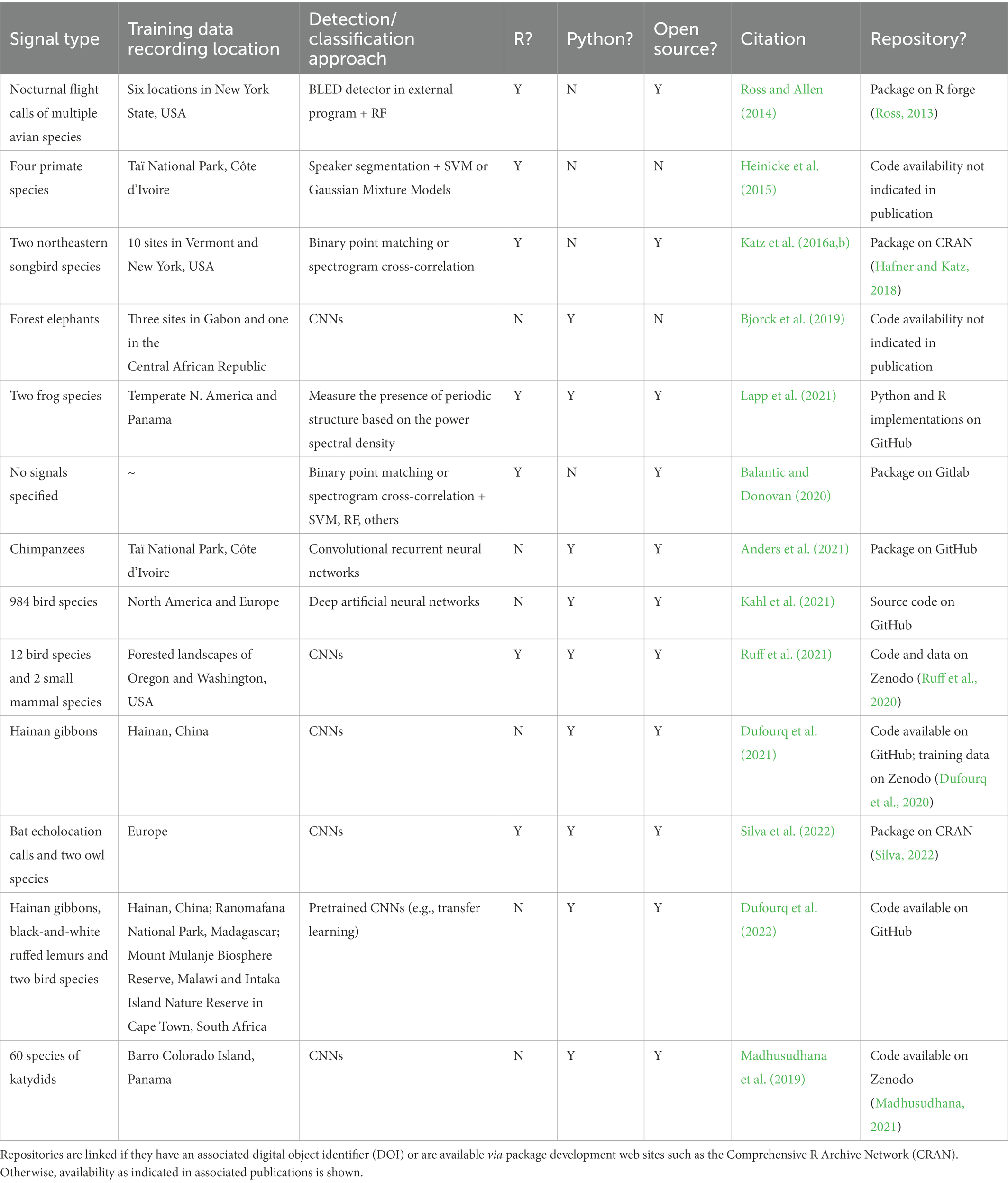
Table 1. Summary of existing approaches that use R or Python for the automated detection/classification of acoustic signals from terrestrial PAM data.
Recently, a workflow was developed that provided a graphical interface through a Shiny application and RStudio for the automated detection of acoustic signals, with the automated detection and classification done using a deep convolutional neural network (CNN) implemented in Python (Ruff et al., 2021). Another R package utilizes deep learning for the automated detection of bat echolocation calls; this package also relies on CNNs implemented in Python (Silva et al., 2022). Deep learning approaches are promising, but they often require large amounts of training data, which can be challenging to obtain, particularly for rare animals or signals (Anders et al., 2021). In addition, training deep learning models may require extensive computational power and specialized hardware (Dufourq et al., 2022); effective training of deep learning models also generally requires a high level of domain knowledge (Hodnett et al., 2019).
Feature extraction
An often necessary step for classification of acoustic signals (unless using deep learning or spectrogram cross-correlation) is feature extraction, wherein the digital waveform is reduced to a meaningful number of informative acoustic features. Traditional approaches relied on manual feature extraction from the spectrogram, but this method requires substantial effort from human observers, which means it is not optimal for automated approaches. Early automated approaches utilized feature sets such as Mel-frequency cepstral coefficients; MFCCs (Heinicke et al., 2015), a feature extraction method originally designed for human speech applications (Han et al., 2006; Muda et al., 2010). Despite their relative simplicity, MFCCs can be used to effectively distinguish between female Northern grey gibbon individuals (Clink et al., 2018a), terrestrial and underwater soundscapes (Dias et al., 2021), urban soundscapes (Noviyanti et al., 2019), and even the presence or absence of queen bees in a bee hive (Soares et al., 2022). Although the use of MFCCs as features for distinguishing between individuals in other gibbon species has been limited, the many documented cases of vocal individuality across gibbon species (Haimoff and Gittins, 1985; Haimoff and Tilson, 1985; Sun et al., 2011; Wanelik et al., 2012; Feng et al., 2014) indicate that MFCCs will most likely be effective features for discriminating individuals of other gibbon species. There are numerous other options for feature extraction, including automated generation of spectro-temporal features for sound events (Sueur et al., 2008; Ross and Allen, 2014) and calculating a set of acoustic indices (Huancapaza Hilasaca et al., 2021).
Other approaches rely on spectrogram images and treat sound classification as an image classification problem (Lucio et al., 2015; Wäldchen and Mäder, 2018; Zottesso et al., 2018). For many of the current deep learning approaches, the input for the classification is the spectrogram, which can be on the linear or Mel-frequency scale (reviewed in Stowell, 2022). An approach that has gained traction in recent years is the use of embeddings, wherein a pre-trained convolutional neural network (CNN), for example, using ‘Google’s AudioSet’ dataset (Gemmeke et al., 2017), is used to create a set of informative, representative features. A common way to do this is to remove the final classification layer from the pre-trained network, which leaves a high-dimensional feature representation of the acoustic data (Stowell, 2022). This approach has been used successfully in numerous ecoacoustic applications (Sethi et al., 2020, 2022; Heath et al., 2021).
Training, validation, and test datasets
When doing automated detection of animal calls, the number and diversity of training data samples must be taken into consideration to minimize false positives (where the system falsely classifies the signal as the signal of interest) and false negatives (e.g., missed opportunities), where the system fails to detect the signal of interest. To avoid overfitting — a phenomenon that occurs when model performance is not generalizable to data that was not included in the training dataset — it is essential to separate data into training, validation, and test sets (Heinicke et al., 2015; Mellinger et al., 2016). The training dataset is the sample of data that was used to fit the model, the validation set is used to provide an unbiased evaluation of a model fit on the training dataset while tuning model hyperparameters, and the test dataset is the sample of data used to provide an unbiased evaluation of a final model fit. Some commonly used metrics include precision (the proportion of detections that are true detections) and recall (the proportion of actual calls that are successfully detected; Mellinger et al., 2016). Often, these metrics are converted to false alarm rates, such as the rate of false positives per hour, which can help guide decisions about the detection threshold. In addition, when doing automated detection and classification, it is common to use a threshold (such as the probability assigned to a classification by a machine learning algorithm) to make decisions about rejecting or accepting a detection (Mellinger et al., 2016). Varying these thresholds will result in changes to false-positive and the proportion of missed calls. These can be plotted with receiver operating curves (ROC; Swets, 1964) or detection error tradeoff curves (DET; Martin et al., 1997).
PAM of gibbons
Gibbons are pair-living, territorial small apes that regularly emit species- and sex-specific long-distance vocalizations that can be heard >1 km in a dense forest (Mitani, 1984, 1985; Geissmann, 2002; Clarke et al., 2006). All but one of the approximately 20 gibbon species are classified as Endangered or Critically Endangered, making them an important target for conservation efforts (IUCN, 2022). Gibbons are often difficult to observe visually in the forest canopy but relatively easy to detect acoustically (Mitani, 1985), which makes them ideal candidates for PAM. Indeed, many early studies relied on human observers listening to calling gibbons to estimate group density using fixed-point counts (Brockelman and Srikosamatara, 1993; Hamard et al., 2010; Phoonjampa et al., 2011; Kidney et al., 2016). To date, relatively few gibbon species have been monitored using PAM, including the Hainan gibbon in China (Dufourq et al., 2021), yellow-cheeked gibbons in Vietnam (Vu and Tran, 2019, 2020), and Northern grey gibbons (Hylobates funereus) on Malaysian Borneo (Clink et al., 2020b). However, this will undoubtedly change over the next few years with increased interest and accessibility of equipment and analytical tools needed for effective PAM of gibbon species across Southeast Asia.
Most gibbon species have two types of long-distance vocalizations. Male solo is the term used for male vocalizations emitted while vocalizing alone, and duets are the coordinated vocal exchange between the adult male and female of the pair (Cowlishaw, 1992, 1996). Gibbons generally call in the early morning, with male gibbon solos starting earlier than the duets (Clink et al., 2020b). In the current paper, we focused our analysis on a call type in the female contribution to the duet, known as the great call, for two reasons. First, the structure of the great call is highly stereotyped, individually distinct (Terleph et al., 2015; Clink et al., 2017), of longer duration than other types of gibbon vocalizations, and the males tend to be silent during the female great call, which facilitates better automated detection. Second, most acoustic density estimation techniques focus on duets, as females rarely sing if they are not in a mated pair (Mitani, 1984). In contrast, males will solo whether in a mated pair or drifters (Brockelman and Srikosamatara, 1993), which means automated detection of the female call will be more relevant for density estimation (Kidney et al., 2016) using PAM. Northern grey gibbon females have been shown to emit individually distinct calls (Clink et al., 2017, 2018a), and these calls can be discriminated well using both supervised and unsupervised methods (Clink and Klinck, 2021).
Individual vocal signatures and PAM
A major hurdle in the implementation of many PAM applications is the fact that individual identity is unknown, as data are collected in the absence of a human observer. In particular, density estimation using PAM data would greatly benefit from the ability to infer the number of individuals in the survey area from acoustic data (Stevenson et al., 2015). The location of the calling animal can infer individual identity. Still, precise acoustic localization that relies on the time difference of arrival (TDOA) of a signal at multiple autonomous recording units can be logistically and analytically challenging (Wijers et al., 2021). Another way that individual identity can be inferred from acoustic data is through individually distinct vocal signatures. Individual vocal signatures have been identified across a diverse range of taxonomic groups (Darden et al., 2003; Gillam and Chaverri, 2012; Kershenbaum et al., 2013; Favaro et al., 2016). Most studies investigating individual signatures use supervised methods, wherein the identity of the calling individual is known, but see Sainburg et al. (2020) for unsupervised applications on individual vocal signatures. Identifying the number of individuals based on acoustic differences from PAM data remains a challenge, as unsupervised approaches must be used since the data are, by definition, collected in the absence of human observers (Clink and Klinck, 2021; Sadhukhan et al., 2021).
Overview of the automated detection/classification workflow
This workflow complements existing R packages for acoustic analysis, such as tuneR (Ligges et al., 2016), seewave (Sueur et al., 2008), warbleR (Araya-Salas and Smith-Vidaurre, 2017), and monitoR (Katz et al., 2016b), and contributes functionalities for automated detection and classification using support vector machine, SVM (Meyer et al., 2017) and random forest, RF (Liaw and Wiener, 2002) algorithms. Automated detection of signals in this workflow follows nine main steps: (1) Create labeled training, validation, and test datasets; (2) identify potential sound events using a band-limited energy detector; (3) data reduction and feature extraction of sound events using Mel-frequency cepstral coefficients; MFCCs (Han et al., 2006; Muda et al., 2010); (4) train machine learning algorithms on the training dataset (5) classify the sound events in the validation dataset using trained machine learning algorithms and calculate performance metrics on the validation dataset to find optimal settings; (6) use a manually labeled test dataset to evaluate model performance; (7) run the detector/classifier over the entire dataset (once the optimal settings have been identified); (8) verify all detections and remove false positives; and (9) use the validated output from the detector/classifier for inference (Figure 1).
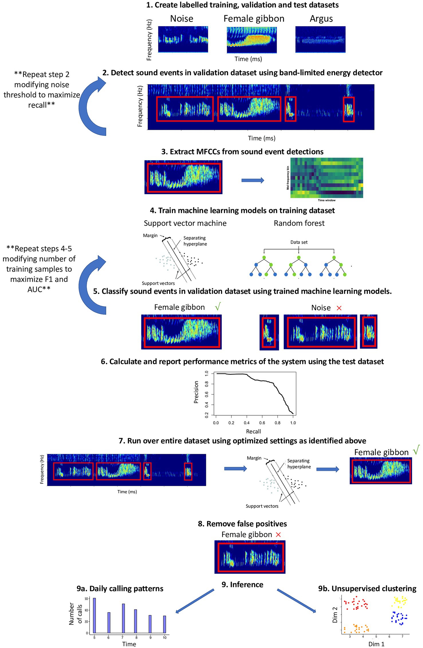
Figure 1. Schematic of automated detection/classification workflow presented in the current study. See the text for details about each step.
When training the system, it is important to use data that will not be used in the subsequent testing phase, as this may artificially inflate accuracy estimates (Heinicke et al., 2015). Creating labeled datasets and subsequent validation of detections to remove false positives requires substantial input and investment by trained analysts; this is the case for all automated detection approaches, even those that utilize sophisticated deep learning approaches. In addition, automated approaches generally require substantial investment in modifying and tuning parameters to identify optimal settings. Therefore, although automated approaches substantially reduce processing time relative to manual review, they still require high levels of human investment throughout the process.
Objectives
We have three main objectives with this manuscript. Although more sophisticated methods of automated detection that utilize deep learning approaches exist (e.g., Dufourq et al., 2021, 2022; Wang et al., 2022), these methods generally require substantial training datasets and are not readily available for users of the R programming environment (R Core Team, 2022). However, (see Silva et al., 2022) for a comprehensive deep-learning R package that relies heavily on Python. We aim to provide an open-source, step-by-step workflow for the automated detection and classification of Northern grey gibbon (H. funereus; hereafter gibbons) female calls using readily available machine learning algorithms in the R programming environment. The results of our study will provide an important benchmark for automated detection/classification applications for gibbon female great calls. We also test whether a post-processing step that utilizes unsupervised clustering can help improve the performance of our system, namely if this approach can help further differentiate between true and false positives. Lastly, as there have been relatively few studies of gibbons that utilize automated detection methods to address a well-defined research question (but see Dufourq et al., 2021 for an example on Hainan gibbons), we aimed to show how PAM can be used to address two different research questions. Specifically, we aim to answer the questions: (1) can we use unsupervised approaches to estimate how many female individuals (or clusters) there are in our study area, and (2) can this approach be used to investigate temporal patterns of gibbon calling activity? We utilized affinity propagation clustering to estimate the number of females (or clusters) in our dataset (Dueck, 2009). This unsupervised clustering algorithm has been shown to be useful for identifying the number of gibbon females in a labeled dataset (Clink and Klinck, 2021). To investigate temporal patterns of calling activity, we compared estimates derived from our automated system to those obtained using manual annotations from LTSAs by a human observer (Clink et al., 2020b).
Materials and methods
Data collection
Acoustic data were collected using first-generation Swift recorders (Koch et al., 2016) developed by the K. Lisa Yang Center for Conservation Bioacoustics at the Cornell Lab of Ornithology. The sensitivity of the used microphones was −44 (+/−3) dB re 1 V/Pa. The microphone’s frequency response was not measured but is assumed to be flat (+/− 2 dB) in the frequency range 100 Hz to 7.5 kHz. The analog signal was amplified by 40 dB and digitized (16-bit resolution) using an analog-to-digital converter (ADC) with a clipping level of −/+ 0.9 V. Recordings were saved as consecutive two-hour Waveform Audio File Format (WAV) with a size of approximately 230 MB. We recorded using a sampling rate of 16 kHz, giving a Nyquist frequency of 8 kHz, which is well above the range of the fundamental frequency of Northern grey gibbon calls (0.5 to 1.6 kHz). We deployed eleven Swift autonomous recording units spaced on a 750-m grid encompassing an area of approximately 3 km2 in the Danum Valley Conservation Area, Sabah, Malaysia (4°57′53.00″N, 117°48′18.38″E) from February 13–April 21, 2018. We attached recorders to trees at approximately 2-m height and recorded continuously over a 24-h period.
Source height (Darras et al., 2016) and presumably recorder height can influence the detection range of the target signal, along with the frequency range of the signal, levels of ambient noise in the frequency range of interest, topography, and source level of the calling animal (Darras et al., 2018). Given the monetary and logistical constraints for placing recorders in the canopy, we opted to place the recorders at a lower height. Our estimated detection range is approximately 500 meters using the settings described below (Clink and Klinck, 2019), and future work investigating the effect of recorder height on detection range will be informative. Danum Valley Conservation Area encompasses approximately 440 km2 of lowland dipterocarp forest and is considered ‘aseasonal’ as it does not have distinct wet and dry seasons like many tropical forest regions (Walsh and Newbery, 1999). Gibbons are less likely to vocalize if there was rain the night before, although rain appears to have a stronger influence on male solos than coordinated duets (Clink et al., 2020b). The reported group density of gibbons in the Danum Valley Conservation Area is ~4.7 per km2 (Hanya and Bernard, 2021), and the home range size of two groups was reported as 0.33 and 0.34 km2 (33 and 34 ha; Inoue et al., 2016).
We limited our analysis to recordings taken between 06:00 and 11:00 local time, as gibbons tend to restrict their calling to the early morning hours (Mitani, 1985; Clink et al., 2020b), which resulted in a total of over 4,500 h of recordings for the automated detection. See Clink et al. (2020b) for a detailed description of the study design and Figure 2 for a study area map. On average, the gibbon duets at this site are 15.1 min long (range = 1.6–55.4 min) (Clink et al., 2020b). The duets are comprised of combinations of notes emitted by both the male and female, often with silent gaps of varying duration between the different components of the duet. The variability of note types and silent intervals in the duet would make training an automated detector/classifier system to identify any component of the duet a challenge (especially in the absence of a lot of training data). In addition, focusing on a certain call type within the longer vocalization is the established approach for automated detection/classification of gibbon vocalizations (Dufourq et al., 2021). Therefore, our automated detection/classification approach focused on the female great call. See Figure 3 for a representative spectrogram of a Northern grey gibbon duet and female great calls within the duet.
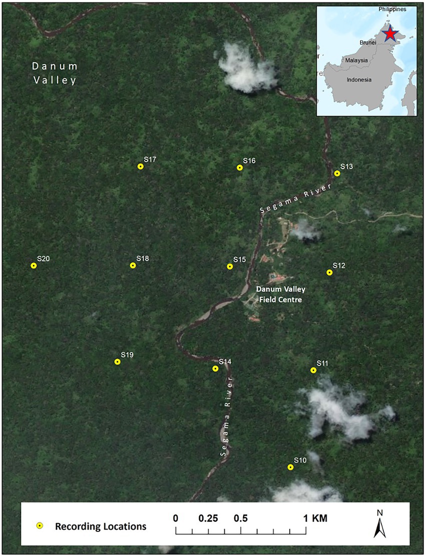
Figure 2. Map of recording locations of Swift autonomous recording units in Danum Valley Conservation Area, Sabah, Malaysia.
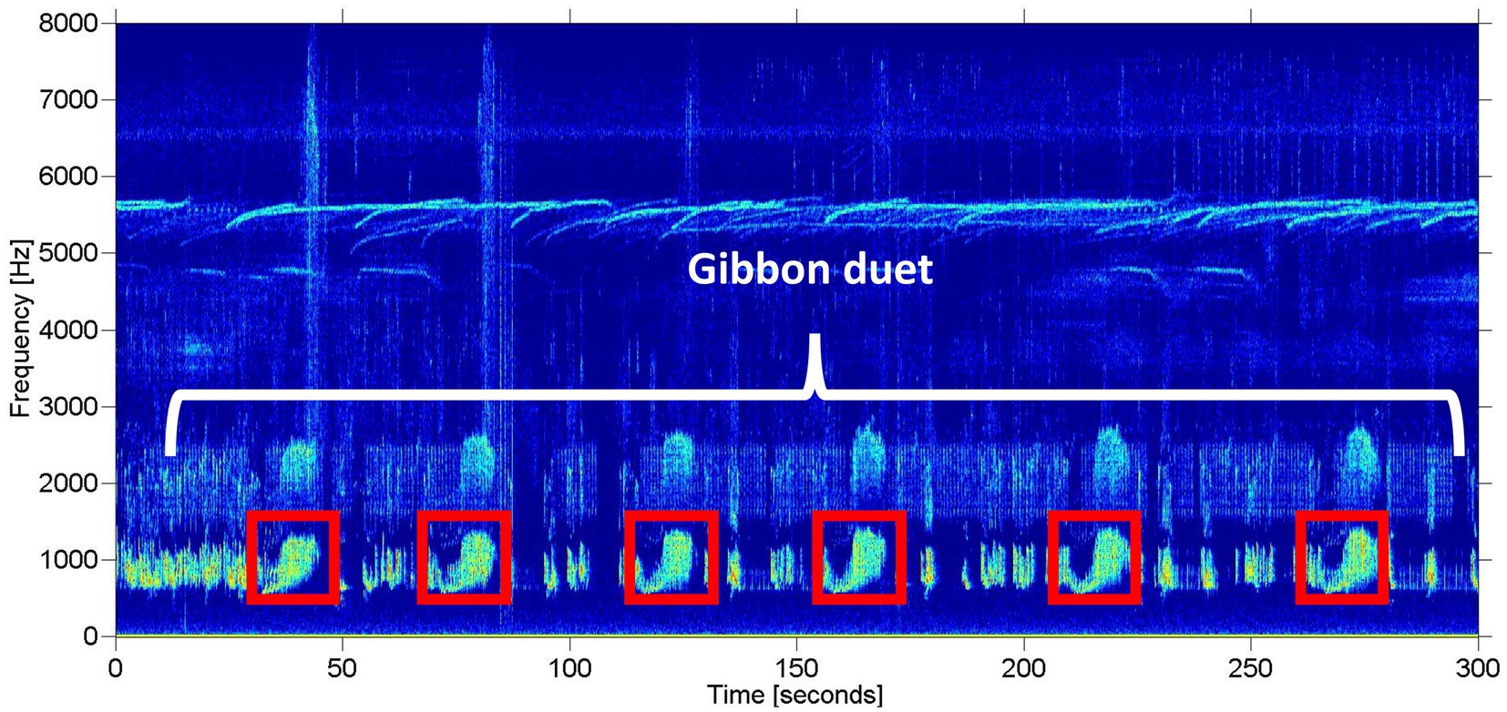
Figure 3. Representative spectrogram of a Northern grey gibbon duet recorded in Danum Valley Conservation Area, Sabah, Malaysia. The white bracket indicates a portion of the gibbon duet (also known as a bout), and the red boxes indicate unique great calls emitted by the gibbon female. The spectrogram was created using the Matlab-based program Triton (Wiggins, 2003).
Creating a labeled training dataset
It is necessary to validate automated detection and classification systems using different training and test datasets (Heinicke et al., 2015). We randomly chose approximately 500 h of recordings to use for our training dataset and used a band-limited energy detector (settings described below) to identify potential sounds of interest in the gibbon frequency range, which resulted in 1,439 unique sound events. The subsequent sound events were then annotated by a single observer (DJC) using a custom-written function in R to visualize the spectrograms into the following categories: great argus pheasant (Argusianus argus) long and short calls (Clink et al., 2021), helmeted hornbills (Rhinoplax vigil), rhinoceros hornbills (Buceros rhinoceros), female gibbons and a catch-all “noise” category. For simplicity of training the machine learning algorithms, we converted our training data into two categories: “female gibbon” or “noise,” and subsequently trained binary classifiers, although the classifiers can also deal with multi-class classification problems. The binary noise class contained all signals that were not female gibbon great calls, including great argus pheasants and hornbills. To investigate how the number of training data samples influences our system’s performance, we randomly subset our training data into batches of 10, 20, 40, 80, 160, 320, and 400 samples of each category (female gibbon and noise) over 10 iterations each. We were also interested to see how the addition of high-quality focal recordings influenced the performance, so we added 60 female gibbon calls collected during focal recordings from previous field seasons (Clink et al., 2018b) to a set of training data. We compared the performance of the detection/classification system using random iterations to the training dataset containing all the training data samples (n = 1,439) and the dataset with the female calls added.
Sound event detection
Detectors are commonly used to isolate potential sound events of interest from background noise (Delacourt and Wellekens, 2000; Davy and Godsill, 2002; Lu et al., 2003). In this workflow, we identified potential sound events based on band-limited energy summation (Mellinger et al., 2016). For the band-limited energy detector (BLED), we first converted the 2-h recordings to a spectrogram (made with a 1,600-point (100 ms) Hamming window (3 dB bandwidth = 13 Hz), with 0% overlap and a 2,048-point DFT) using the package “seewave” (Sueur et al., 2008). We filtered the spectrogram to the frequency range of interest (in the case of Northern grey gibbons 0.5–1.6 kHz). For each non-overlapping time window, we calculated the sum of the energy across frequency bins, which resulted in a single value for each 100 ms time window. We then used the “quantile” function in base R to calculate the threshold value for signal versus noise. We ran early experiments using different quantile values and found that using the 15th quantile gave the best recall for our signal of interest. We then considered any events which lasted for 5 s or longer to be detections. Note that settings for the band-limited energy detector, MFCCs, and machine learning algorithms can be modified; we modified the detector and MFCC settings as independent steps in early experiments. We found in early experiments that modifying the quantile values and the duration of the detections influenced the performance of our system, so we suggest practitioners adopting this method experiment with modifying these settings to fit their system.
Supervised classification
We were interested in testing the performance of secondary classifiers —support vector machine (SVM) or random forest (RF) — for classifying our detected sound events. To train the classifiers, we used the training datasets outlined above and calculated Mel-frequency cepstral coefficients (MFCCs) for each of the labeled sound events using the R package “tuneR” (Ligges et al., 2016). We calculated MFCCs focusing on the fundamental frequency range of female gibbon calls (0.5–1.6 kHz). We focused on the fundamental frequency range because harmonics are generally not visible in the recordings unless the animals were very close to the recording units. As the duration of sound events is variable, and machine learning classification approaches require feature vectors of equal length, we averaged MFCCs over time windows. First, we divided each sound event into 8 evenly spaced time windows (with the actual length of each window varying based on the duration of the event) and calculated 12 MFCCs along with the delta coefficients for each time window (Ligges et al., 2016). We appended the duration of the event onto the MFCC vector, resulting in a vector for each sound event of length 177. We then used the E1071 package (Meyer et al., 2017) to train a SVM and the “randomForest” package (Liaw and Wiener, 2002) to train a RF, respectively. Each algorithm assigned each sound event to a class (“female gibbon” or “noise”) and returned an associated probability. For SVM, we set “cross = 25,” meaning that we used 25-fold cross-validation, set the kernel to “radial,” and used the “tune” parameter to find optimal settings for the cost and gamma parameters. For the random forest algorithm, we used the default settings apart from setting the number of trees = 10,000.
Validation and test datasets
We annotated our validation and test datasets using a slightly different approach than we used for the training data. We did this because our system utilizes a band-limited energy detector. If we simply labeled the resulting clips (like we did with the training data), our performance metrics would not account for the detections that were missed initially by the detector. Therefore, to create our test and validation datasets, one observer (DJC) manually annotated 48 randomly chosen hours of recordings taken from different recorders and times across our study site using spectrograms created in Raven Pro 1.6. Twenty-four hours were used for validation, and the remaining 24 h were used as a test dataset to report the final performance metrics of the system. For each sound file, we identified the begin and end time of any female gibbon vocalization. We also labeled calls as high quality (wherein the full structure of the call was visible in the spectrogram and there were no overlapping bird calls or other background noises) or low quality (wherein the call was visible in the spectrogram, but the full structure was not, or there was overlapping with another calling animal/noise). As the detector isolates sound events based on energy in a certain frequency band, sometimes the start time of the detection does not align exactly with the annotated start time of the call; therefore, when calculating the performance metrics we considered sound events that started 4 s before the annotations or 2 s after the annotations to be a match.
We evaluated our system using five different metrics using the R package ‘ROCR’ (Sing et al., 2005) to calculate precision, recall, and false alarm rate. We were interested to see how the performance of our classifiers varied when we changed the probability threshold, so we calculated the area under the precision-recall curves, which shows the trade-off between the rate of false-positives and false-negatives at different probability thresholds. We calculated the area under the receiver operating characteristic curve (AUC) for each machine learning algorithm and training dataset configuration. We also calculated the F1 score, as it integrates both precision and recall information into the metric.
We used a model selection approach to test for the effects of training data and machine learning algorithm on our performance metrics (AUC), so we created as series of two linear models using the R package “lme4” (Bates et al., 2017). The first model we considered, the null model, had only AUC as the outcome, with no predictor variables. The second model, which we considered the full model, contained the machine learning algorithm (SVM or RF) and training data category as predictors. We used the Akaike information criterion (AIC) to compare the fit of the two models to our data, implemented in the “bbmle” package (AICctab adjusted for small sample sizes; Bolker, 2014). We chose the settings that maximized AUC and the F1-score for the subsequent analysis of the full dataset (described below).
Verification workflow
The optimal detector/classifier settings for our two main objectives were slightly different. For our first objective, wherein we wanted to compare patterns of vocal activity based on the output of our automated detector to patterns identified using human-annotated datasets (Clink et al., 2020b), we aimed to maximize recall while also maintaining an acceptable number of false positives. In early tests, we found that using a smaller quantile threshold (0.15) for the BLED detector improved recall. One observer (IK) manually verified all detections using a custom function in R that allows observers to quickly view spectrograms and verify detections. Although duet bouts contain many great calls, we considered instances where at least one great call was detected during each hour as the presence of a duet. We then compared our results to those identified using a human observer and calculated the percent of annotated duets the automated system detected. To compare the two distributions, we used a Kolmogorov–Smirnov test implemented using the ‘ks.test’ function in the R version 4.2.1 programming environment (R Core Team, 2022). We first converted the times to “Unix time” (the number of seconds since 1970-01-01 00:00:00 UTC; Grolemund and Wickham, 2011) so that we had continuous values for comparison. We used a non-parametric test as we did not assume a normal distribution of our data.
For the objective wherein we used unsupervised clustering to quantify the number of females (clusters) in our dataset, we needed higher quality calls in terms of signal-to-noise ratio (SNR) and overall structure. This is because the use of MFCCs as features for discriminating among individuals is highly dependent on SNR (Spillmann et al., 2017). For this objective, we manually omitted all detections that did not follow the species-specific structure with longer introductory notes that transition into rapidly repeating trill notes and only used detections with a probability >0.99 as assigned by the SVM (Clink et al., 2017).
Unsupervised clustering
We used unsupervised clustering to investigate the tendency to cluster in: (A) the verified detections containing true and false positives after running the detector/classifier over our entire dataset: and (B) female calls that follow the species-specific structure of the great call wherein different clusters may reflect different individuals. We used affinity propagation clustering, a state-of-the-art unsupervised approach (Dueck, 2009) that has been used successfully in a few bioacoustics applications, including anomaly detection in a forest environment (Sethi et al., 2020) and clustering of female gibbon calls with known identity (Clink and Klinck, 2021). Our previous work showed that out of three unsupervised algorithms compared, affinity propagation clustering returned a number of clusters that matched the number of known female individuals in our dataset most closely (Clink and Klinck, 2021). Input preferences for the affinity propagation clustering algorithm can vary the number of clusters returned. We initially used an adaptive approach wherein we varied the input preference from 0.1 to 1 in increments of 0.1 (indicated by “q” in the “APCluster” R package; Bodenhofer et al., 2011) and calculated silhouette coefficients using the “cluster” package (Maechler et al., 2019). We found that the optimal q identified in this manner led to an unreasonably high number of clusters for the true/false positives, so we set q = 0.1, resulting in fewer clusters.
We input an MFCC vector for each sound event into the affinity propagation clustering algorithm. For the true/false positives, we calculated the MFCCs slightly differently than outlined above, as fewer features resulted in better clustering. Instead of creating a standardized number of time windows for each event, we calculated MFCCs for each sound event using the default settings (wintime = 0.025, hoptime = 0.01, and numcep = 12). We then took the mean and standard deviation for each Mel-frequency band and the delta coefficients, resulting in 48 unique values for each sound event. We also included the duration of the signal. For the true and false positive detections, we used normalized mutual information (NMI) as an external validation measure implemented in the ‘aricode’ package (Chiquet and Rigaill, 2019). NMI provides a value between 0 and 1, with 1 indicating a perfect match between two sets of labels (Xuan et al., 2010). For clustering of the high-quality female calls, we used the adaptive approach to find the optimal value of q. We used the standard number of MFCC windows approach as outlined above.
To visualize clustering in our dataset, we used a uniform manifold learning technique (UMAP) implemented in the R package ‘umap’ (Konopka, 2020). UMAP is a data reduction and visualization approach that has been used to visualize differences in forest soundscapes (Sethi et al., 2020), taxonomic groups of neotropical birds (Parra-Hernández et al., 2020), and female gibbon great calls (Clink and Klinck, 2021).
Data availability
A tutorial, annotated code, and all data needed to recreate figures presented in the manuscript are available on GitHub.1 Access to raw sound files used for training and testing can be granted by request to the corresponding author.
Results
Training data and algorithm influence performance
The classification accuracy of SVM for the training dataset containing all samples was 98.82%, and the accuracy of the RF was 97.85%. We found that the number of training data samples and the selected machine learning algorithm substantially influenced the performance of our detector/classifier using the validation dataset (Table 2). Using an AIC model selection approach, we found that the model with AUC as an outcome and with the machine learning algorithm and training data category as predictors performed much better than the null model (ΔAICc = 11.2; 100% of model weight). When using AUC as the metric, we found that SVM performed slightly better than RF, and performance normalized when the number of training samples was greater than n = 160 (Figure 4). We also found that the model with F1 score as an outcome and machine learning algorithm and training data category as predictors performed much better than the null model (ΔAICc = 34,730.6; 100% of model weight; Figure 4). Again, SVM performed better than RF, but in this case, the training dataset that contained all the samples (n = 433 female calls and n = 1,006 noise events) or all the samples plus extra female calls performed better (Figure 4). There were noticeable differences in the performance of the two algorithms regarding F1 score across different probability thresholds (Figure 5). SVM had a higher performance at higher probability thresholds, whereas performance for RF had the highest F1 value when the probability threshold was 0.60. We decided to use the SVM algorithm with all the training samples for our full analysis. We used the 24-h test dataset to calculate the final performance metrics of our system. We found that the highest F1 score (0.78) was when the probability threshold was 0.90, precision was 0.88, and recall was 0.71.
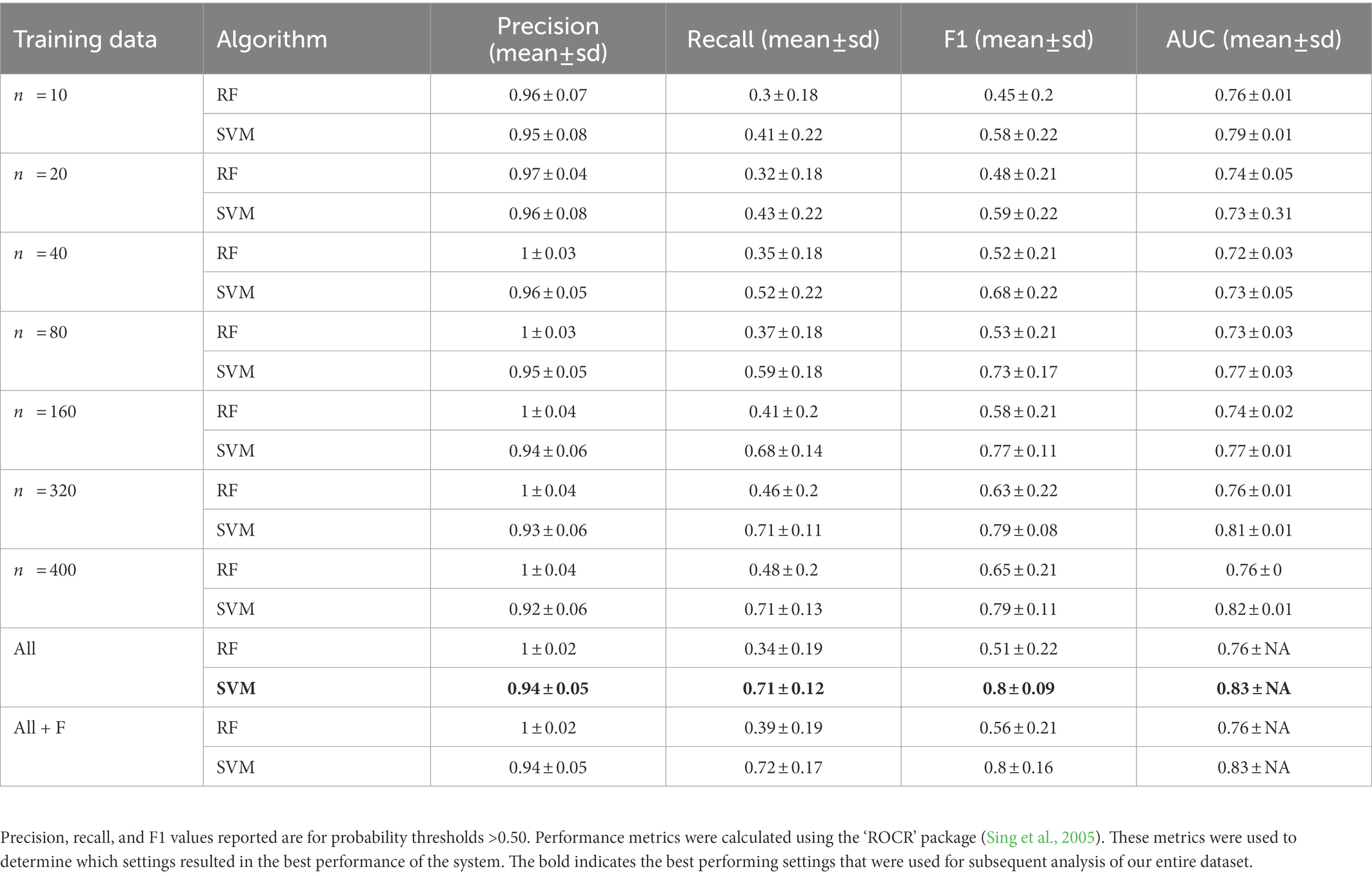
Table 2. Summary of precision, recall, F1, and area under the curve (AUC) calculated using the validation dataset for random subsets of training data compared to the full training dataset and the full dataset augmented with female great calls.
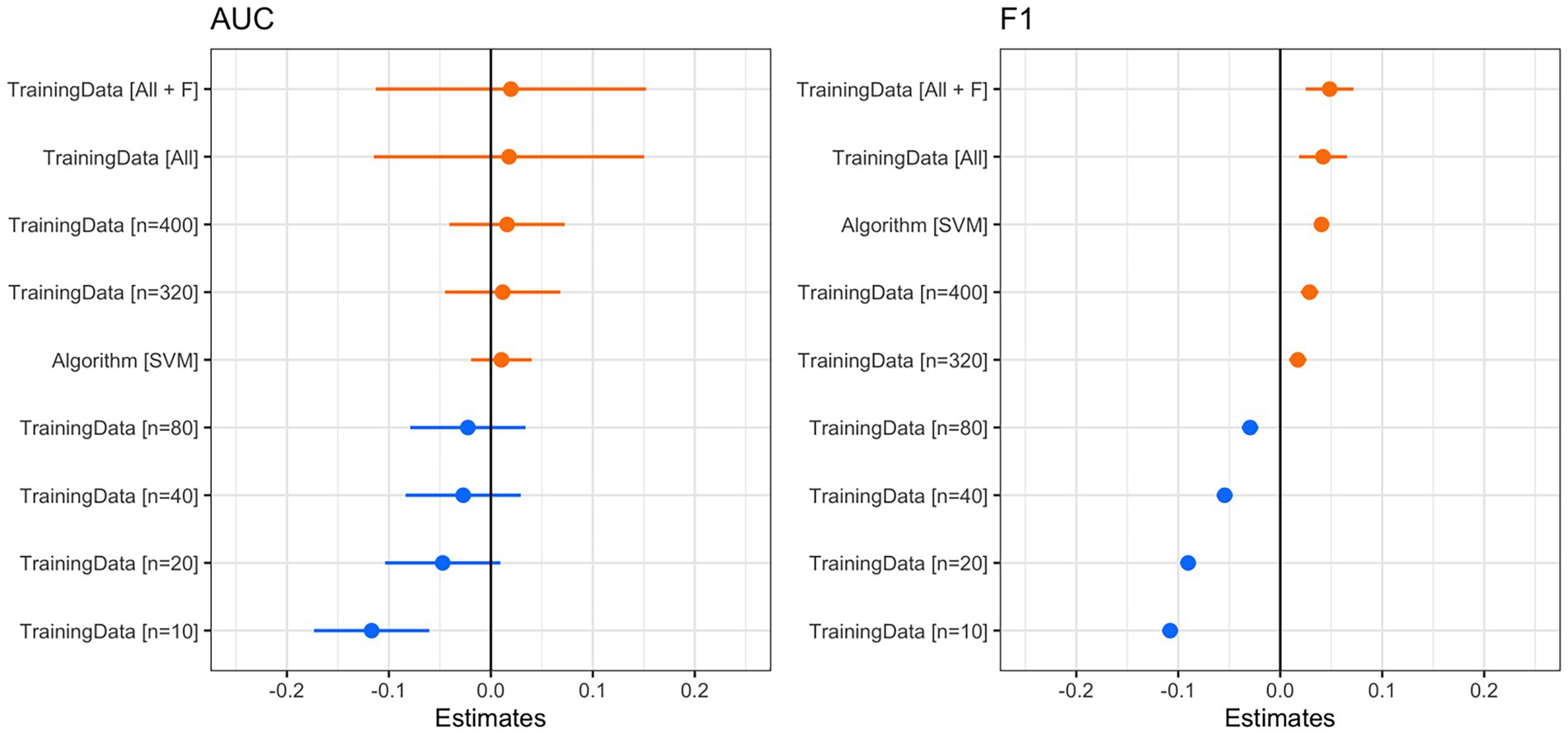
Figure 4. Coefficient plots from the linear model with AUC (left) or F1 score (right) as the outcome and training data category and machine learning algorithm as predictors. Using AIC, we found that both models performed substantially better than the null model. For both coefficient plots, the reference training data category is n = 160. We considered predictors to be reliable if the confidence intervals did not overlap zero. For AUC (left), training data samples smaller than n = 160 had a slightly negative impact on AUC, whereas a larger number of training data samples had a slightly positive impact. Note that the confidence intervals overlap zero, so these can be interpreted only as trends. The use of the SVM algorithm had a slightly positive effect on AUC. For the F1 score (right), the number of training samples had a reliable effect on the F1 score. When samples were less than n = 160, the F1 score was lower. When there were more samples, the F1 score was higher. SVM also had a reliably positive effect on the F1 score.
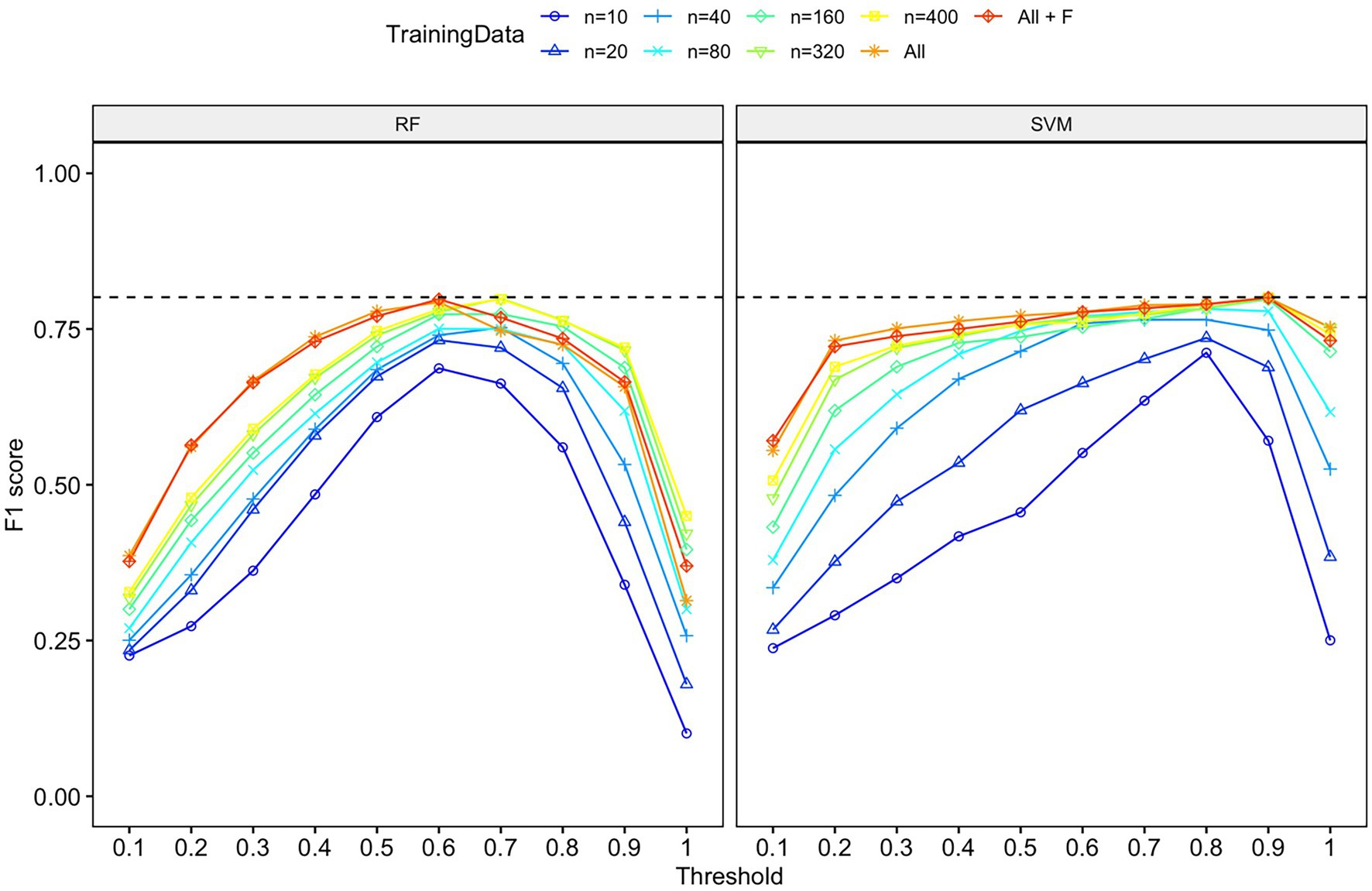
Figure 5. F1-score for each machine learning algorithm (RF or SVM), probability threshold category, and training data category. Both algorithms had comparable performance in terms of F1 score, although the probability threshold with the highest F1 score differed. The dashed line indicates the highest F-1 score (0.80) for both algorithms on the validation dataset.
Comparison of an automated system to human annotations
We used the SVM algorithm and all training data samples to run over our full dataset resulting in 4,771 detections, of which 3,662 were true positives and 1109 were false positives (precision = 0.77). A histogram showing the distributions of automatically detected calls and manually annotated calls is shown in Figure 6. A Kolmogorov–Smirnov test indicated that the two distributions were not significantly different D = 0.07, p > 0.05.
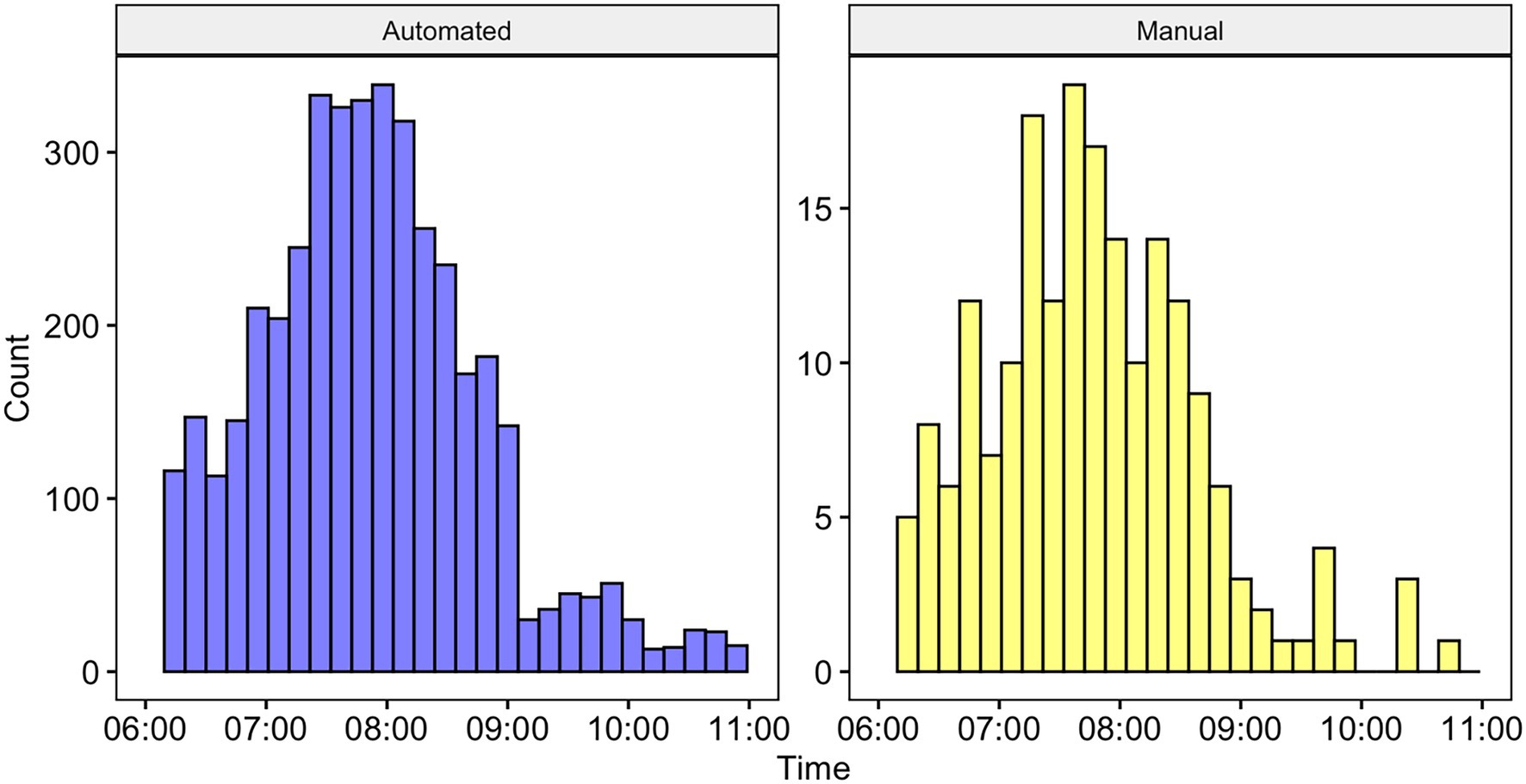
Figure 6. Histogram showing the number of calls detected by time using the automated system (left) and manually annotated by a human observer (right). Note that the differences in axes are due to the detections for the automated system being at the call level, whereas the annotations were at the bout level (and bouts are comprised of multiple calls). There was no statistically significant difference between the two distributions (see text for details).
Unsupervised clustering
We used unsupervised clustering to investigate the tendency to cluster in true/false positives and high-quality female calls. For our first aim, we used affinity propagation clustering to differentiate between true and false positives after we used our detection/classification system. We did not find that affinity propagation clustering effectively separated false positives, as the NMI score was close to zero (NMI = 0.03). Although there were only two classes in our dataset (true and false positives), the clustering results indicated 53 distinct clusters. Supervised classification accuracy using SVM for true and false positives was ~95%. UMAP projections of the true and false positive detections are shown in Figure 7. For our second aim, we used affinity propagation clustering to investigate the tendency to cluster in the high-quality female calls detected by our system (n = 194). Using adaptive affinity propagation clustering, we found that setting q = 0.2 resulted in the highest silhouette coefficient (0.18) and returned ten unique clusters. UMAP projections of female calls are shown in Figure 8. Histograms indicating the number of calls from each recorder assigned to each cluster by the affinity propagation algorithm are shown in Figure 9.
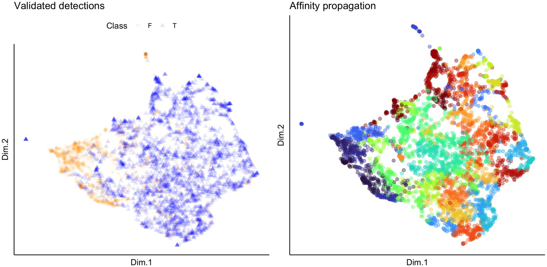
Figure 7. UMAP projections indicating validated detections (left) and cluster assignment by affinity propagation clustering (right). Each point represents a detection, and the colors in the plot on the left indicate whether the detection was a true (T; indicated by the blue triangles) or false (F; indicated by the orange circles) positive. The colors in the plot on the right indicate which of the 53 clusters returned by the affinity propagation clustering algorithm the detection was assigned to.
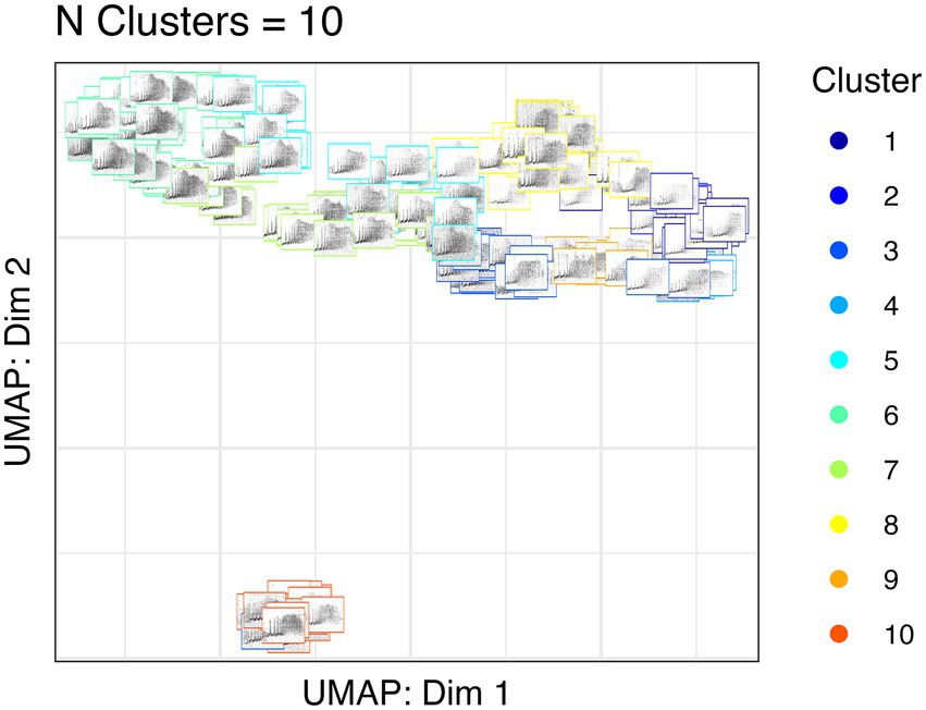
Figure 8. UMAP projections of Northern grey gibbon female calls. The location of each spectrogram indicates the UMAP projection of the call, and the border color indicates cluster assignment by affinity propagation clustering.
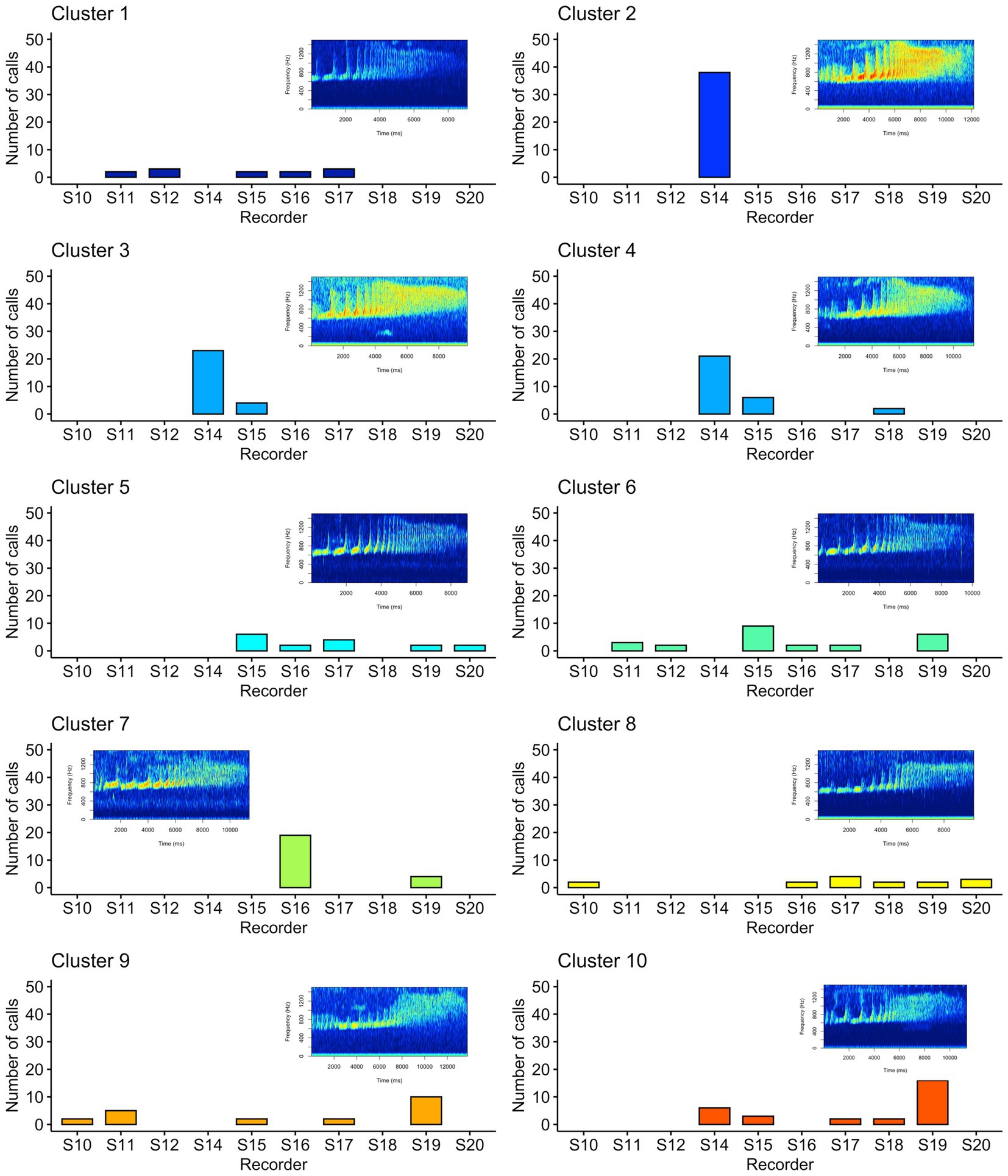
Figure 9. Histograms showing the number of calls assigned to each cluster by the affinity propagation algorithm. Each panel indicates one of the clusters as assigned by affinity propagation clustering, the x-axis indicates the associated recording unit where the call was detected, and the y-axis indicates the number of calls for each cluster and recorder. The spectrograms shown exemplify each cluster assigned by the affinity propagation clustering algorithm.
Discussion
We show that using open-source R packages, a detector and classifier can be developed with an acceptable performance that exceeds that of previously published automated detector/classifiers for primate calls [e.g., Diana monkey F1 based on reported precision and recall = 65.62 (Heinicke et al., 2015)]. However, the performance of this system (maximum F1 score = 0.78) was below some reported deep learning approaches [e.g., F1 score = 90.55 for Hainan gibbons (Dufourq et al., 2021), F1 score = ~87.5 for owl species (Ruff et al., 2021), F1 score = 87.0 for bats (Silva et al., 2022)]. In addition, we found that temporal patterns of calling based on our automated system matched those of the human annotation approach. We also tested whether using an unsupervised approach (affinity propagation clustering) could help further distinguish true and false positive detections but found that the clustering results (n = 53 clusters) did not differentiate true and false positives in any meaningful way. Visual inspection of the false positives indicated that many of them were overlapping with great argus pheasants, or were other parts of the gibbon duet or solo. A majority of the false positives were male solo phrases, and these vocalization types contain rapidly repeating notes in the same frequency range as the female gibbon call. Lastly, we applied unsupervised clustering to a reduced dataset of validated detections of female calls that followed the species-specific call structure and found evidence for ten unique clusters. Inspection of spatial patterns of distribution of the clusters indicates that the clusters do not correlate with female identity.
Calls versus bouts
Our analysis focused on one call type within the gibbon duet: the female great call. We did this for practical reasons, as female calls tend to be stereotyped and follow a species- and sex-specific pattern. In addition, females rarely call alone, which means the presence of the female call can be used to infer the presence of a pair of gibbons. Also, most acoustic survey methods focus on the duet for the reasons described above, and generally, only data on the presence or absence of a duet bout at a particular time and location are needed (Brockelman and Srikosamatara, 1993; Kidney et al., 2016). When calculating the performance of our automated detection/classification system, we focused on the level of the call, as this is a common way to evaluate the performance of automated systems (Dufourq et al., 2020). Finally, when comparing temporal patterns of calling behavior, we compared to an existing dataset of annotations at the level of the duet bout. We did this because annotating duet bouts using LTSAs is much more efficient than annotating each individual call for the entire dataset. However, for certain applications such as individual vocal signatures, the analysis necessarily focuses on individual calls within a bout.
Comparison of ML algorithms
We found that SVM performed slightly better than RF in most metrics reported (except precision). However, RF had a comparable classification accuracy to SVM on the training dataset (SVM accuracy = 98.82% and RF accuracy = 97.85% for all training data samples). This reduced performance can be attributed to the substantially lower recall of RF relative to SVM, despite RF having higher precision in many cases (data summarized in Table 2). The precision of SVM decreased slightly as we increased the number of training samples, which may be due to increased variability in the training data samples that influenced the algorithm’s precision. We did not see that the precision of RF decreased with an increased number of training samples, but RF recall remained low regardless of the amount of training data. These patterns are reflected in differences in the F1 scores across probabilities for both algorithms.
The tolerable number of false positives, or the minimum tolerable recall of the system, will depend heavily on the research question. For example, when modeling occupancy, it may be important that no calls are missed, and hence, a higher recall would be desirable. But, for studies that focus more on the behavioral ecology of the calling animals (Clink et al., 2020a,b), it may be important for the detector to identify calls with a low amount of false positives but less important if the detector misses many low signal-to-noise calls. Therefore, in some cases where high precision is desired but recall is less important, RF may be a better choice. It is also possible that tuning the RF (as we did with SVM) may result in better performance. However, we did not do this as it is generally agreed that RF works well using default values of the hyperparameters (Probst et al., 2019).
Influence of training data
We found that the AUC and F1 metrics normalized when using 160 samples of training data or more for each of the two classes (gibbon female and noise). However, using all training data or data augmented with female calls resulted in better F1 scores. The training datasets that contained all the samples and added females were unbalanced and contained many more noise samples than female calls. Including more diverse noise samples lead to better performance in this system, and both RF and SVM handle unbalanced datasets effectively. It is important to note that although we found performance normalized when training with 160 calls or more, this number does not account for the additional number of calls needed for validation and training. Therefore, the total number of calls or observations to effectively train and subsequently evaluate the performance of the system will be >160 calls. We realize that compiling a dataset of 160 or more calls for rare sound events from elusive species may be unrealistic. We found that our in our system including as few as 40 calls allowed for acceptable performance (F1 score for SVM = 0.70), so the approach could be potentially used successfully with a much smaller training dataset.
In addition, our training, validation, and test datasets came from different recording units, times of day, and multiple territories of different gibbon groups. Including 40 calls from the same recorder and same individual would presumably not be as effective as including calls from different individuals and recording locations. A full discussion of the effective preparation of datasets for machine learning is out of the scope of the present paper, but readers are urged to think carefully about the preparation of acoustic datasets for automated detection and aim to include samples from a diverse number of recording locations, individuals and time of day. Transfer learning which utilizes pre-trained convolutional neural networks for different classification problems than the model was originally trained, provides another alternative for small datasets, with transfer learning providing up to an 82% F1 score with small datasets (Dufourq et al., 2022). Future work that compares the approach presented here with transfer learning will be highly informative.
Unsupervised clustering to distinguish true/false positives
We did not find that affinity propagation clustering helped further differentiate true and false positives in our dataset, despite being able to differentiate between the two classes using supervised methods with ~95% accuracy. As noted above, many of the false positives were phrases from male solos, and these phrases are highly variable in note order and note sequence (Clink et al., 2020a), which may have led to the high number of clusters observed. The NMI score was close to zero, indicating a lack of accordance between the unsupervised cluster assignments and the true labels. These types of unsupervised approaches have been fruitful in distinguishing among many different types of acoustic signals, including soundscapes (Sethi et al., 2020), bird species (Parra-Hernández et al., 2020), and gibbon individuals (Clink and Klinck, 2021). We extracted MFCCs for all sound events focusing on the relevant frequency range for female gibbon great calls. As detections were based on band-limited energy summation in this frequency range, extracting MFCCs in this frequency range was a logical choice. We did early experiments where we summarized the extracted MFCCs in different ways and slightly modified the frequency range. We did not find that these early experiments led to better separation of true and false positives. Therefore, we conclude that the use of MFCCs and affinity propagation clustering is not an effective way to differentiate between true and false positives in our dataset. It is possible that using different features may have led to different results, and embeddings from convolutional neural networks as features (e.g., Sethi et al., 2020) or the use of low dimentional latent space projections learned from the spectrograms (Sainburg et al., 2020) are promising future directions.
Unsupervised clustering of validated gibbon female calls
The ability to distinguish between individuals based on their vocalizations is important for many different PAM applications, and population density estimation in particular (Augustine et al., 2018, 2019). The home range size of two gibbon pairs in our population was previously reported to be about 0.34 km2 (34 ha; Inoue et al., 2016), but within gibbon populations, the home range size can vary substantially (Cheyne et al., 2019), making it difficult to know exactly how many pairs were included in our study area. In another study, gibbon group density was reported as 4.7 groups per km2; the discrepancy between this value and home range size estimates provided by Inoue et al. (2016) is presumably due to the fact that the studies were measuring different parameters (density vs. home range) and the fact that home ranges can overlap, even in territorial species. Therefore, based on conservative estimates of gibbon density and home range size, up to 12 pairs may occur in our 3 km2 study area.
Our unsupervised approach using affinity propagation clustering on high-quality female calls returned ten unique clusters. We showed that affinity propagation clustering consistently returned a similar number of clusters to the actual number of individuals in a different dataset (Clink and Klinck, 2021). However, an inspection of the histograms in Figure 9 shows that some clusters appear to have strong spatial patterns (e.g., only appearing on a few recorders in close spatial proximity), whereas others appear on many recorders. In some cases, the same clusters appear on recorders that are >1.5 km apart — a presumably larger distance than the width of a gibbon home range — therefore, it seems unlikely that these clusters are associated with female identity. When using unsupervised approaches, it is common practice to assign each cluster to the class that contains the highest number of observations, and we showed affinity propagation clustering reliably returned a number of clusters that matched the number of individuals in the dataset, but often ‘misclassified’ calls to the wrong cluster/individual (Clink and Klinck, 2021). Importantly, our previous work was done on high-quality, focal recordings with a substantial amount of preprocessing to ensure the calls were comparable (e.g., did not contain shorter introductory notes or overlap with the male). In the present study, we manually screened calls to ensure they followed the species-specific structure and were relatively high-quality, but the limitations of PAM data (collected using an omnidirectional, relatively inexpensive microphone, and at variable distances to the calling animals) may preclude effective unsupervised clustering of individuals.
We conclude that more work needs to be done before we can reliably use unsupervised methods to estimate the number of individuals in a study area. Our current ability to utilize these approaches to return the number of individuals reliably is presently limited, especially because there is not a lot of information regarding the stability of individual signatures over time; but (see Feng et al., 2014). Future work that utilizes labeled training datasets collected using PAM data to train classifiers that can subsequently predict new individuals (e.g., an approach similar to that presented in; Sadhukhan et al., 2021) will help further our ability to identify unknown individuals from PAM data.
Generalizability of the system
Gibbon female calls are well-suited for automated detection and classification as they are loud and highly stereotyped, and gibbon females tend to call often. During a particular calling bout, they emit multiple calls, allowing for ample training data. Although gibbon female calls are individually distinct (Clink et al., 2017, 2018a), the differences between individuals were not sufficient to preclude detection and classification using our system. Importantly, the fact that gibbon female calls tend to be of longer duration (> 6-s) than many other signals in the frequency range meant that the duration of the signal could be used as an effective metric to reject nonrelevant signals. The generalizability of our methods to other systems/datasets will depend on a variety of conditions, in particular, the signal-to-noise ratio of the call(s) of interest, type and variability of background noise, the amount of stereotypy in the calls of interest, and the amount of training data that can be obtained to train the system. Future applications that apply this approach to other gibbon species, or compare this approach with deep learning techniques, will be important next steps to determine the utility and effectiveness of automated detection approaches for other taxa.
Future directions
Due to the three-step design of our automated detection, classification, and unsupervised clustering approach, modifying the system at various stages should be relatively straightforward. In particular, using MFCCs as features was a logical approach given how well MFCCs work to distinguish among gibbon calls [this paper and Clink et al. (2018a)]. However, it is possible that using different types of feature sets may result in even better performance of the automated system. As mentioned above, the use of embeddings from pre-trained convolutional neural networks is a possibility. In addition, the supervised classification algorithms included in our approach were not optimized; the RF algorithm, in particular, was implemented using the default values set by the algorithm developers. Therefore, further tuning and optimization of the algorithms may also influence the performance. Lastly, this approach was developed using training, validation, and test data from one site (Danum Valley Conservation Area). Future work investigating the performance of this system in other locations with (presumably) different types of ambient noise will be informative.
Conclusion
Here we highlight how the open-source R-programming environment can be used to process and visualize acoustic data collected using autonomous recorders that are often programmed to record continuously for long periods of time. Even the most sophisticated machine learning algorithms are never 100% accurate or precise and will return false positives or negatives (Bardeli et al., 2010; Heinicke et al., 2015; Keen et al., 2017), which is also the case with human observers, but this is rarely quantified statistically (Heinicke et al., 2015). We hope this relatively simple automated detection/classification approach will serve as a useful foundation for practitioners interested in automated acoustic analysis methods. We also show that unsupervised approaches need further work and refinement before they can be reliably used to distinguish between different data classes recorded using autonomous recording units. Given the importance of being able to distinguish among individuals for numerous types of PAM applications, this should be a high-priority area for future research.
Data availability statement
The raw data supporting the conclusions of this article will be made available by the authors, without undue reservation.
Ethics statement
Institutional approval was provided by Cornell University (IACUC 2017-0098).
Author contributions
DC, AA, and HK conceived the ideas and designed the methodology. DC and IK annotated and validated data. DC and IK led the writing of the manuscript. All authors contributed critically to the drafts and gave final approval for publication.
Funding
DC acknowledges the Fulbright ASEAN Research Award for U.S. Scholars for providing funding for the field research.
Acknowledgments
The authors thank the two reviewers who provided valuable feedback that greatly improved the manuscript. We thank the makers of the packages “randomforest,” “e1017,” “seewave,” “signal,” and “tuneR,” on which this workflow relies extensively. We thank Yoel Majikil for his assistance with data collection for this project.
Conflict of interest
The authors declare that the research was conducted in the absence of any commercial or financial relationships that could be construed as a potential conflict of interest.
Publisher’s note
All claims expressed in this article are solely those of the authors and do not necessarily represent those of their affiliated organizations, or those of the publisher, the editors and the reviewers. Any product that may be evaluated in this article, or claim that may be made by its manufacturer, is not guaranteed or endorsed by the publisher.
Footnotes
References
Anders, F., Kalan, A. K., Kühl, H. S., and Fuchs, M. (2021). Compensating class imbalance for acoustic chimpanzee detection with convolutional recurrent neural networks. Eco. Inform. 65:101423. doi: 10.1016/j.ecoinf.2021.101423
Araya-Salas, M., and Smith-Vidaurre, G. (2017). warbleR: an R package to streamline analysis of animal acoustic signals. Methods Ecol. Evol. 8, 184–191. doi: 10.1111/2041-210X.12624
Augustine, B. C., Royle, J. A., Kelly, M. J., Satter, C. B., Alonso, R. S., Boydston, E. E., et al. (2018). Spatial capture–recapture with partial identity: an application to camera traps. Ann. Appl. Stat. 12, 67–95. doi: 10.1214/17-AOAS1091
Augustine, B. C., Royle, J. A., Murphy, S. M., Chandler, R. B., Cox, J. J., and Kelly, M. J. (2019). Spatial capture–recapture for categorically marked populations with an application to genetic capture–recapture. Ecosphere 10:e02627. doi: 10.1002/ecs2.2627
Balantic, C., and Donovan, T. (2020). AMMonitor: remote monitoring of biodiversity in an adaptive framework with r. Methods Ecol. Evol. 11, 869–877. doi: 10.1111/2041-210X.13397
Bardeli, R., Wolff, D., Kurth, F., Koch, M., Tauchert, K. H., and Frommolt, K. H. (2010). Detecting bird sounds in a complex acoustic environment and application to bioacoustic monitoring. Pattern Recogn. Lett. 31, 1524–1534. doi: 10.1016/j.patrec.2009.09.014
Bates, D., Maechler, M., Bolker, B. M., and Walker, S. (2017). lme4: Linear Mixed-Effects Models Using “Eigen” and S4. R package version 1.1-13. Available at: http://keziamanlove.com/wp-content/uploads/2015/04/StatsInRTutorial.pdf https://cran.r-project.org/web/packages/lme4/lme4.pdf (Accessed January 23, 2023).
Bjorck, J., Rappazzo, B. H., Chen, D., Bernstein, R., Wrege, P. H., and Gomes, C. P. (2019). Automatic detection and compression for passive acoustic monitoring of the african forest elephant. Proc. AAAI Conf. Artific. Intellig. 33, 476–484. doi: 10.1609/aaai.v33i01.3301476
Bodenhofer, U., Kothmeier, A., and Hochreiter, S. (2011). APCluster: an R package for affinity propagation clustering. Bioinformatics 27, 2463–2464. doi: 10.1093/bioinformatics/btr406
Bolker, B. M. (2014). bbmle: tools for general maximum likelihood estimation. Available at: http://cran.stat.sfu.ca/web/packages/bbmle/ (Accessed January 23, 2023).
Brockelman, W. Y., and Srikosamatara, S. (1993). Estimation of density of gibbon groups by use of loud songs. Am. J. Primatol. 29, 93–108. doi: 10.1002/ajp.1350290203
Cheyne, S. M., Capilla, B. R., K, A., Supiansyah,, Adul,, Cahyaningrum, E., et al. (2019). Home range variation and site fidelity of Bornean southern gibbons [Hylobates albibarbis] from 2010–2018. PLoS One 14, e0217784–e0217713. doi: 10.1371/journal.pone.0217784
Chiquet, J., and Rigaill, G. (2019). Aricode: efficient computations of standard clustering comparison measures. Available at: https://cran.r-project.org/package=aricode (Accessed January 23, 2023).
Clarke, E., Reichard, U. H., and Zuberbühler, K. (2006). The syntax and meaning of wild gibbon songs. PLoS One 1:e73. doi: 10.1371/journal.pone.0000073
Clink, D. J., Bernard, H., Crofoot, M. C., and Marshall, A. J. (2017). Investigating individual vocal signatures and small-scale patterns of geographic variation in female bornean gibbon (Hylobates muelleri) great calls. Int. J. Primatol. 38, 656–671. doi: 10.1007/s10764-017-9972-y
Clink, D. J., Crofoot, M. C., and Marshall, A. J. (2018a). Application of a semi-automated vocal fingerprinting approach to monitor Bornean gibbon females in an experimentally fragmented landscape in Sabah, Malaysia. Bioacoustics 28, 193–209. doi: 10.1080/09524622.2018.1426042
Clink, D. J., Grote, M. N., Crofoot, M. C., and Marshall, A. J. (2018b). Understanding sources of variance and correlation among features of Bornean gibbon (Hylobates muelleri) female calls. J. Acoust. Soc. Am. 144, 698–708. doi: 10.1121/1.5049578
Clink, D. J., Groves, T., Ahmad, A. H., and Klinck, H. (2021). Not by the light of the moon: investigating circadian rhythms and environmental predictors of calling in Bornean great argus. PLoS One 16:e0246564. doi: 10.1371/journal.pone.0246564
Clink, D. J., Hamid Ahmad, A., and Klinck, H. (2020a). Brevity is not a universal in animal communication: evidence for compression depends on the unit of analysis in small ape vocalizations. R. Soc. Open Sci. 7. doi: 10.1098/rsos.200151
Clink, D. J., Hamid Ahmad, A., and Klinck, H. (2020b). Gibbons aren’t singing in the rain: presence and amount of rainfall influences ape calling behavior in Sabah, Malaysia. Sci. Rep. 10:1282. doi: 10.1038/s41598-020-57976-x
Clink, D. J., and Klinck, H. (2019). A case study on Bornean gibbons highlights the challenges for incorporating individual identity into passive acoustic monitoring surveys. J. Acoust. Soc. Am. 146:2855. doi: 10.1121/1.5136908
Clink, D. J., and Klinck, H. (2021). Unsupervised acoustic classification of individual gibbon females and the implications for passive acoustic monitoring. Methods Ecol. Evol. 12, 328–341. doi: 10.1111/2041-210X.13520
Cowlishaw, G. (1992). Song function in gibbons. Behaviour 121, 131–153. doi: 10.1163/156853992X00471
Cowlishaw, G. (1996). Sexual selection and information content in gibbon song bouts. Ethology 102, 272–284. doi: 10.1111/j.1439-0310.1996.tb01125.x
Dahake, P. P., and Shaw, K. (2016). Speaker dependent speech emotion recognition using MFCC and support vector machine. in International Conference on Automatic Control and Dynamic Optimization Techniques (ICACDOT), 1080–1084.
Darden, S. K., Dabelsteen, T., and Pedersen, S. B. (2003). A potential tool for swift fox (Vulpes velox) conservation: individuality of long-range barking sequences. J. Mammal. 84, 1417–1427. doi: 10.1644/BEM-031
Darras, K., Furnas, B., Fitriawan, I., Mulyani, Y., and Tscharntke, T. (2018). Estimating bird detection distances in sound recordings for standardizing detection ranges and distance sampling. Methods Ecol. Evol. 9, 1928–1938. doi: 10.1111/2041-210X.13031
Darras, K., Pütz, P., Rembold, K., and Tscharntke, T. (2016). Measuring sound detection spaces for acoustic animal sampling and monitoring. Biol. Conserv. 201, 29–37. doi: 10.1016/j.biocon.2016.06.021
Davy, M., and Godsill, S. (2002). Detection of abrupt spectral changes using support vector machines an application to audio signal segmentation. 2002 IEEE International Conference on Acoustics, Speech, and Signal Processing Orlando, FL: IEEE. 1313–1316.
Deichmann, J. L., Acevedo-Charry, O., Barclay, L., Burivalova, Z., Campos-Cerqueira, M., d’Horta, F., et al. (2018). It’s time to listen: there is much to be learned from the sounds of tropical ecosystems. Biotropica 50, 713–718. doi: 10.1111/btp.12593
Delacourt, P., and Wellekens, C. J. (2000). DISTBIC: a speaker-based segmentation for audio data indexing. Speech Comm. 32, 111–126. doi: 10.1016/S0167-6393(00)00027-3
Dias, F. F., Pedrini, H., and Minghim, R. (2021). Soundscape segregation based on visual analysis and discriminating features. Eco. Inform. 61:101184. doi: 10.1016/j.ecoinf.2020.101184
Dueck, D. (2009). Affinity propagation: Clustering data by passing messages. Toronto, ON, Canada: University of Toronto, 144.
Dufourq, E., Batist, C., Foquet, R., and Durbach, I. (2022). Passive acoustic monitoring of animal populations with transfer learning. Eco. Inform. 70:101688. doi: 10.1016/j.ecoinf.2022.101688
Dufourq, E., Durbach, I., Hansford, J. P., Hoepfner, A., Ma, H., Bryant, J. V., et al. (2021). Automated detection of Hainan gibbon calls for passive acoustic monitoring. Remote Sens. Ecol. Conserv. 7, 475–487. doi: 10.1002/rse2.201
Dufourq, E., Durbach, I., Hansford, J. P., Hoepfner, A., Ma, H., Bryant, J. V., et al. (2020). Automated detection of Hainan gibbon calls for passive acoustic monitoring. doi: 10.5281/zenodo.3991714.
Favaro, L., Gili, C., Da Rugna, C., Gnone, G., Fissore, C., Sanchez, D., et al. (2016). Vocal individuality and species divergence in the contact calls of banded penguins. Behav. Process. 128, 83–88. doi: 10.1016/j.beproc.2016.04.010
Feng, J.-J., Cui, L.-W., Ma, C.-Y., Fei, H.-L., and Fan, P.-F. (2014). Individuality and stability in male songs of cao vit gibbons (Nomascus nasutus) with potential to monitor population dynamics. PLoS One 9:e96317. doi: 10.1371/journal.pone.0096317
Geissmann, T. (2002). Duet-splitting and the evolution of gibbon songs. Biol. Rev. 77, 57–76. doi: 10.1017/S1464793101005826
Gemmeke, J. F., Ellis, D. P., Freedman, D., Jansen, A., Lawrence, W., Moore, R. C., et al. (2017). Audio set: an ontology and human-labeled dataset for audio events. in 2017 IEEE international conference on acoustics, speech and signal processing (ICASSP), Piscataway, NJ IEEE 776–780.
Gibb, R., Browning, E., Glover-Kapfer, P., and Jones, K. E. (2018). Emerging opportunities and challenges for passive acoustics in ecological assessment and monitoring. Methods Ecol. Evol. 10, 169–185. doi: 10.1111/2041-210X.13101
Gillam, E. H., and Chaverri, G. (2012). Strong individual signatures and weaker group signatures in contact calls of Spix’s disc-winged bat, Thyroptera tricolor. Anim. Behav. 83, 269–276. doi: 10.1016/j.anbehav.2011.11.002
Grolemund, G., and Wickham, H. (2011). Dates and times made easy with lubridate. J. Stat. Softw. 40, 1–25. doi: 10.18637/jss.v040.i03
Hafner, S. D., and Katz, J. (2018). monitoR: acoustic template detection in R. Available at: http://www.uvm.edu/rsenr/vtcfwru/R/?Page=monitoR/monitoR.htm (Accessed January 23, 2023).
Haimoff, E., and Gittins, S. (1985). Individuality in the songs of wild agile gibbons (Hylobates agilis) of Peninsular Malaysia. Am. J. Primatol. 8, 239–247. doi: 10.1002/ajp.1350080306
Haimoff, E., and Tilson, R. (1985). Individuality in the female songs of wild kloss’ gibbons (Hylobates klossii) on Siberut Island, Indonesia. Folia Primatol. 44, 129–137. doi: 10.1159/000156207
Hamard, M., Cheyne, S. M., and Nijman, V. (2010). Vegetation correlates of gibbon density in the peat-swamp forest of the Sabangau catchment, Central Kalimantan, Indonesia. Am. J. Primatol. 72, 607–616. doi: 10.1002/ajp.20815
Han, W., Chan, C.-F., Choy, C.-S., and Pun, K.-P. (2006). An efficient MFCC extraction method in speech recognition. in 2006 IEEE International Symposium on Circuits and Systems, Piscataway, NJ IEEE 4.
Hanya, G., and Bernard, H. (2021). Interspecific encounters among diurnal primates in Danum Valley, Borneo. Int. J. Primatol. 42, 442–462. doi: 10.1007/s10764-021-00211-9
Heath, B. E., Sethi, S. S., Orme, C. D. L., Ewers, R. M., and Picinali, L. (2021). How index selection, compression, and recording schedule impact the description of ecological soundscapes. Ecol. Evol. 11, 13206–13217. doi: 10.1002/ece3.8042
Heinicke, S., Kalan, A. K., Wagner, O. J. J., Mundry, R., Lukashevich, H., and Kühl, H. S. (2015). Assessing the performance of a semi-automated acoustic monitoring system for primates. Methods Ecol. Evol. 6, 753–763. doi: 10.1111/2041-210X.12384
Hill, A. P., Prince, P., Piña Covarrubias, E., Doncaster, C. P., Snaddon, J. L., and Rogers, A. (2018). AudioMoth: evaluation of a smart open acoustic device for monitoring biodiversity and the environment. Methods Ecol. Evol. 9, 1199–1211. doi: 10.1111/2041-210X.12955
Hodnett, M., Wiley, J. F., Liu, Y. H., and Maldonado, P. (2019). Deep Learning with R for Beginners: Design Neural Network Models in R 3.5 Using TensorFlow, Keras, and MXNet. Birmingham Packt Publishing Ltd.
Huancapaza Hilasaca, L. M., Gaspar, L. P., Ribeiro, M. C., and Minghim, R. (2021). Visualization and categorization of ecological acoustic events based on discriminant features. Ecol. Indic. 126:107316. doi: 10.1016/j.ecolind.2020.107316
Inoue, Y., Sinun, W., and Okanoya, K. (2016). Activity budget, travel distance, sleeping time, height of activity and travel order of wild east Bornean Grey gibbons (Hylobates funereus) in Danum Valley conservation area. Raff. Bull. Zool. 64, 127–138.
IUCN (2022). The IUCN Red List of Threatened Species. The IUCN Red List of Threatened Species. Available at: https://www.iucnredlist.org ().
Kahl, S., Wood, C. M., Eibl, M., and Klinck, H. (2021). BirdNET: a deep learning solution for avian diversity monitoring. Eco. Inform. 61:101236. doi: 10.1016/j.ecoinf.2021.101236
Kalan, A. K., Mundry, R., Wagner, O. J. J., Heinicke, S., Boesch, C., and Kühl, H. S. (2015). Towards the automated detection and occupancy estimation of primates using passive acoustic monitoring. Ecol. Indic. 54, 217–226. doi: 10.1016/j.ecolind.2015.02.023
Kalan, A. K., Piel, A. K., Mundry, R., Wittig, R. M., Boesch, C., and Kühl, H. S. (2016). Passive acoustic monitoring reveals group ranging and territory use: a case study of wild chimpanzees (pan troglodytes). Front. Zool. 13:34. doi: 10.1186/s12983-016-0167-8
Katz, J., Hafner, S. D., and Donovan, T. (2016a). Assessment of error rates in acoustic monitoring with the R package monitoR. Bioacoustics 25, 177–196. doi: 10.1080/09524622.2015.1133320
Katz, J., Hafner, S. D., and Donovan, T. (2016b). Tools for automated acoustic monitoring within the R package monitoR. Bioacoustics 25, 197–210. doi: 10.1080/09524622.2016.1138415
Keen, S. C., Shiu, Y., Wrege, P. H., and Rowland, E. D. (2017). Automated detection of low-frequency rumbles of forest elephants: a critical tool for their conservation. J. Acoust. Soc. Am. 141, 2715–2726. doi: 10.1121/1.4979476
Kershenbaum, A., Sayigh, L. S., and Janik, V. M. (2013). The encoding of individual identity in dolphin signature whistles: how much information is needed? PLoS One 8:e77671. doi: 10.1371/journal.pone.0077671
Kidney, D., Rawson, B. M., Borchers, D. L., Stevenson, B. C., Marques, T. A., and Thomas, L. (2016). An efficient acoustic density estimation method with human detectors applied to gibbons in Cambodia. PLoS One 11:e0155066. doi: 10.1371/journal.pone.0155066
Koch, R., Raymond, M., Wrege, P., and Klinck, H. (2016). SWIFT: a small, low-cost acoustic recorder for terrestrial wildlife monitoring applications. in North American Ornithological Conference Washington, DC, 619.
Konopka, T. (2020). Umap: uniform manifold approximation and projection. Available at: https://cran.r-project.org/package=umap (Accessed January 23, 2023).
Lai, J., Lortie, C. J., Muenchen, R. A., Yang, J., and Ma, K. (2019). Evaluating the popularity of R in ecology. Ecosphere 10:e02567. doi: 10.1002/ecs2.2567
Lapp, S., Wu, T., Richards-Zawacki, C., Voyles, J., Rodriguez, K. M., Shamon, H., et al. (2021). Automated detection of frog calls and choruses by pulse repetition rate. Conserv. Biol. 35, 1659–1668. doi: 10.1111/cobi.13718
Lawlor, J., Banville, F., Forero-Muñoz, N.-R., Hébert, K., Martínez-Lanfranco, J. A., Rogy, P., et al. (2022). Ten simple rules for teaching yourself R. PLoS Comput. Biol. 18:e1010372. doi: 10.1371/journal.pcbi.1010372
Ligges, U., Krey, S., Mersmann, O., and Schnackenberg, S. (2016). {tuneR}: analysis of music. Available at: https://r-forge.r-project.org/projects/tuner/
Lu, L., Zhang, H.-J., and Li, S. Z. (2003). Content-based audio classification and segmentation by using support vector machines. Multimed. Syst. 8, 482–492. doi: 10.1007/s00530-002-0065-0
Lucio, D. R., Maldonado, Y., and da Costa, G. (2015). Bird species classification using spectrograms. in 2015 Latin American Computing Conference (CLEI), Arequipa, Peru 1–11.
Madhusudhana, S., Shiu, Y., Klinck, H., Fleishman, E., Liu, X., Nosal, E.-M., et al. (2021). Improve automatic detection of animal call sequences with temporal context. J. R. Soc. Interface 18:20210297. doi: 10.1098/rsif.2021.0297
Madhusudhana, S. K., Symes, L. B., and Klinck, H. (2019). A deep convolutional neural network based classifier for passive acoustic monitoring of neotropical katydids. J. Acoust. Soc. Am. 146:2982. doi: 10.1121/1.5137323
Maechler, M., Rousseeuw, P., Struyf, A., Hubert, M., and Hornik, K. (2019). Cluster: cluster analysis basics and extensions.
Markolf, M., Zinowsky, M., Keller, J. K., Borys, J., Cillov, A., and Schülke, O. (2022). Toward passive acoustic monitoring of lemurs: using an affordable open-source system to monitor Phaner vocal activity and density. Int. J. Primatol. 43, 409–433. doi: 10.1007/s10764-022-00285-z
Marques, T. A., Thomas, L., Martin, S. W., Mellinger, D. K., Ward, J. A., Moretti, D. J., et al. (2013). Estimating animal population density using passive acoustics. Biol. Rev. 88, 287–309. doi: 10.1111/brv.12001
Martin, A., Doddington, G., Kamm, T., Ordowski, M., and Przybocki, M. (1997). The DET curve in assessment of detection task performance. Proc. Eurospeech 4, 1895–1898.
Mellinger, D. K., Roch, M. A., Nosal, E.-M., and Klinck, H. (2016). “Signal processing” in Listening in the Ocean. eds. W. W. Au and M. O. Lammers (Berlin: Springer), 359–409.
Meyer, D., Dimitriadou, E., Hornik, K., Weingessel, A., and Leisch, F. (2017). e1071: Misc functions of the Department of Statistics.
Mielke, A., and Zuberbühler, K. (2013). A method for automated individual, species and call type recognition in free-ranging animals. Anim. Behav. 86, 475–482. doi: 10.1016/j.anbehav.2013.04.017
Mitani, J. C. (1984). The behavioral regulation of monogamy in gibbons (Hylobates muelleri). Behav. Ecol. Sociobiol. 15, 225–229. doi: 10.1007/BF00292979
Mitani, J. C. (1985). Gibbon song duets and intergroup spacing. Behaviour 92, 59–96. doi: 10.1080/0141192032000137321
Muda, L., Begam, M., and Elamvazuthi, I. (2010). Voice recognition algorithms using Mel frequency cepstral coefficient (MFCC) and dynamic time warping (DTW) techniques. J. Comput. 2, 2151–9617. doi: 10.48550/arXiv.1003.4083
Noviyanti, A., Sudarsono, A. S., and Kusumaningrum, D. (2019). Urban soundscape prediction based on acoustic ecology and MFCC parameters. AIP Conf. Proc. 2187:050005. doi: 10.1063/1.5138335
Parra-Hernández, R. M., Posada-Quintero, J. I., Acevedo-Charry, O., and Posada-Quintero, H. F. (2020). Uniform manifold approximation and projection for clustering taxa through vocalizations in a neotropical passerine (rough-legged tyrannulet, Phyllomyias burmeisteri). Animals 10:1406. doi: 10.3390/ani10081406
Pérez-Granados, C., and Schuchmann, K.-L. (2021). Passive acoustic monitoring of the diel and annual vocal behavior of the Black and Gold Howler Monkey. Am. J. Primatol. 83:e23241. doi: 10.1002/ajp.23241
Phoonjampa, R., Koenig, A., Brockelman, W. Y., Borries, C., Gale, G. A., Carroll, J. P., et al. (2011). Pileated gibbon density in relation to habitat characteristics and post-logging forest recovery. Biotropica 43, 619–627. doi: 10.1111/j.1744-7429.2010.00743.x
Probst, P., Wright, M. N., and Boulesteix, A.-L. (2019). Hyperparameters and tuning strategies for random forest. Wiley Interdiscipl. Rev. 9:e1301. doi: 10.1002/widm.1301
R Core Team (2022). R: A Language and Environment for Statistical Computing. Vienna, Austria: R Foundation for Statistical Computing. Available at: https://www.R-project.org/ (Accessed January 23, 2023).
Romero-Mujalli, D., Bergmann, T., Zimmermann, A., and Scheumann, M. (2021). Utilizing DeepSqueak for automatic detection and classification of mammalian vocalizations: a case study on primate vocalizations. Sci. Rep. 11:24463. doi: 10.1038/s41598-021-03941-1
Ross, J. C. (2013). Flightcallr: Classify Night Flight Calls Based on Acoustic Measurements. Available at: https://R-Forge.R-project.org/projects/flightcallr/ (Accessed January 23, 2023).
Ross, J. C., and Allen, P. E. (2014). Random Forest for improved analysis efficiency in passive acoustic monitoring. Eco. Inform. 21, 34–39. doi: 10.1016/j.ecoinf.2013.12.002
Ruff, Z. J., Lesmeister, D. B., Appel, C. L., and Sullivan, C. M. (2020). Convolutional neural network and R-Shiny app for identifying vocalizations in Pacific Northwest forests. doi: 10.5281/zenodo.4092393.
Ruff, Z. J., Lesmeister, D. B., Appel, C. L., and Sullivan, C. M. (2021). Workflow and convolutional neural network for automated identification of animal sounds. Ecol. Indic. 124:107419. doi: 10.1016/j.ecolind.2021.107419
Sadhukhan, S., Root-Gutteridge, H., and Habib, B. (2021). Identifying unknown Indian wolves by their distinctive howls: its potential as a non-invasive survey method. Sci. Rep. 11:7309. doi: 10.1038/s41598-021-86718-w
Sainburg, T., Thielk, M., and Gentner, T. Q. (2020). Finding, visualizing, and quantifying latent structure across diverse animal vocal repertoires. PLoS Comput. Biol. 16:e1008228. doi: 10.1371/journal.pcbi.1008228
Scavetta, R. J., and Angelov, B. (2021). Python and R for the Modern Data Scientist. California, USA: O’Reilly Media, Inc.
Sethi, S. S., Ewers, R. M., Jones, N. S., Orme, C. D. L., and Picinali, L. (2018). Robust, real-time and autonomous monitoring of ecosystems with an open, low-cost, networked device. Methods Ecol. Evol. 9, 2383–2387. doi: 10.1111/2041-210X.13089
Sethi, S. S., Ewers, R. M., Jones, N. S., Sleutel, J., Shabrani, A., Zulkifli, N., et al. (2022). Soundscapes predict species occurrence in tropical forests. Oikos 2022:e08525. doi: 10.1111/oik.08525
Sethi, S. S., Jones, N. S., Fulcher, B. D., Picinali, L., Clink, D. J., Klinck, H., et al. (2020). Characterizing soundscapes across diverse ecosystems using a universal acoustic feature set. Proc. Natl. Acad. Sci. 117, 17049–17055. doi: 10.1073/pnas.2004702117
Shiu, Y., Palmer, K. J., Roch, M. A., Fleishman, E., Liu, X., Nosal, E.-M., et al. (2020). Deep neural networks for automated detection of marine mammal species. Sci. Rep. 10, 1–12. doi: 10.1038/s41598-020-57549-y
Shonfield, J., and Bayne, E. M. (2017). Autonomous recording units in avian ecological research: current use and future applications. Avian Conserv. Ecol. 12:art14. doi: 10.5751/ACE-00974-120114
Silva, B. (2022). soundClass: Sound Classification Using Convolutional Neural Networks. Available at: https://CRAN.R-project.org/package=soundClass (Accessed January 23, 2023).
Silva, B., Mestre, F., Barreiro, S., Alves, P. J., and Herrera, J. M. (2022). soundClass: an automatic sound classification tool for biodiversity monitoring using machine learning. Methods Ecol. Evolut. 13, 2356–2362. doi: 10.1111/2041-210X.13964
Sing, T., Sander, O., Beerenwinkel, N., Lengauer, T., Sing, T., Sander, O., et al. (2005). ROCR: visualizing classifier performance in R. Bioinformatics 21, 3940–3941. doi: 10.1093/bioinformatics/bti623
Soares, B. S., Luz, J. S., de Macêdo, V. F., Silva, R. R. V. E., De Araújo, F. H. D., and Magalhães, D. M. V. (2022). MFCC-based descriptor for bee queen presence detection. Expert Syst. Appl. 201:117104. doi: 10.1016/j.eswa.2022.117104
Spillmann, B., van Schaik, C. P., Setia, T. M., and Sadjadi, S. O. (2017). Who shall I say is calling? Validation of a caller recognition procedure in Bornean flanged male orangutan (Pongo pygmaeus) long calls. Bioacoustics 26, 109–120. doi: 10.1080/09524622.2016.1216802
Stevenson, B. C., Borchers, D. L., Altwegg, R., Swift, R. J., Gillespie, D. M., and Measey, G. J. (2015). A general framework for animal density estimation from acoustic detections across a fixed microphone array. Methods Ecol. Evol. 6, 38–48. doi: 10.1111/2041-210X.12291
Stowell, D. (2022). Computational bioacoustics with deep learning: a review and roadmap. PeerJ 10:e13152. doi: 10.7717/peerj.13152
Sueur, J., Aubin, T., and Simonis, C. (2008). Seewave: a free modular tool for sound analysis and synthesis. Bioacoustics 18, 213–226. doi: 10.1080/09524622.2008.9753600
Sugai, L. S. M., and Llusia, D. (2019). Bioacoustic time capsules: using acoustic monitoring to document biodiversity. Ecol. Indic. 99, 149–152. doi: 10.1016/j.ecolind.2018.12.021
Sugai, L. S. M., Silva, T. S. F., Ribeiro, J. W., and Llusia, D. (2019). Terrestrial passive acoustic monitoring: review and perspectives. Bioscience 69, 15–25. doi: 10.1093/biosci/biy147
Sun, G.-Z., Huang, B., Guan, Z.-H., Geissmann, T., and Jiang, X.-L. (2011). Individuality in male songs of wild black crested gibbons (Nomascus concolor ). Am. J. Primatol. 73, 431–438. doi: 10.1002/ajp.20917
Swets, J. A. (1964). Signal Detection and Recognition by Human Observers: Contemporary Readings. New York, NY: Wiley.
Terleph, T. A., Malaivijitnond, S., and Reichard, U. H. (2015). Lar gibbon (Hylobates lar) great call reveals individual caller identity. Am. J. Primatol. 77, 811–821. doi: 10.1002/ajp.22406
Vu, T. T., and Tran, L. M. (2019). An application of autonomous recorders for gibbon monitoring. Int. J. Primatol. 40, 169–186. doi: 10.1007/s10764-018-0073-3
Vu, T. T., and Tran, D. V. (2020). Using autonomous recorders and bioacoustics to monitor the globally endangered wildlife in the Annamite mountain landscape: a case study with crested argus in Song Thanh Nature Reserve. J. Nat. Conserv. 56:125843. doi: 10.1016/j.jnc.2020.125843
Wäldchen, J., and Mäder, P. (2018). Machine learning for image based species identification. Methods Ecol. Evol. 9, 2216–2225. doi: 10.1111/2041-210X.13075
Walsh, R. P., and Newbery, D. M. (1999). The ecoclimatology of Danum, Sabah, in the context of the world’s rainforest regions, with particular reference to dry periods and their impact. Philos. Trans. R. Soc. Lond. B Biol. Sci 354, 1869–1883. doi: 10.1098/rstb.1999.0528
Wanelik, K. M., Azis, A., and Cheyne, S. M. (2012). Note-, phrase- and song-specific acoustic variables contributing to the individuality of male duet song in the Bornean southern gibbon (Hylobates albibarbis). Primates 54, 159–170. doi: 10.1007/s10329-012-0338-y
Wang, Y., Ye, J., and Borchers, D. L. (2022). Automated call detection for acoustic surveys with structured calls of varying length. Methods Ecol. Evolut. 13, 1552–1567. doi: 10.1111/2041-210X.13873
Wiggins, S. (2003). Autonomous acoustic recording packages (ARPs) for long-term monitoring of whale sounds. Mar. Technol. Soc. J. 37, 13–22. doi: 10.4031/002533203787537375
Wijers, M., Loveridge, A., Macdonald, D. W., and Markham, A. (2021). CARACAL: A versatile passive acoustic monitoring tool for wildlife research and conservation. Bioacoustics 30, 41–57.
Xuan, N., Julien, V., Wales, S., and Bailey, J. (2010). Information theoretic measures for clusterings comparison: variants, properties, normalization and correction for chance. J. Mach. Learn. Res. 11, 2837–2854.
Zeppelzauer, M., Hensman, S., and Stoeger, A. S. (2015). Towards an automated acoustic detection system for free-ranging elephants. Bioacoustics 24, 13–29. doi: 10.1080/09524622.2014.906321
Zottesso, R. H. D., Costa, Y. M. G., Bertolini, D., and Oliveira, L. E. S. (2018). Bird species identification using spectrogram and dissimilarity approach. Eco. Inform. 48, 187–197. doi: 10.1016/j.ecoinf.2018.08.007
Keywords: machine learning, Hylobates, R programing language, signal processing, bioacoustics, Southeast Asia
Citation: Clink DJ, Kier I, Ahmad AH and Klinck H (2023) A workflow for the automated detection and classification of female gibbon calls from long-term acoustic recordings. Front. Ecol. Evol. 11:1071640. doi: 10.3389/fevo.2023.1071640
Edited by:
Marco Gamba, University of Turin, ItalyReviewed by:
Lydia Light, University of North Carolina at Charlotte, United StatesTim Sainburg, University of California, San Diego, United States
Copyright © 2023 Clink, Kier, Ahmad and Klinck. This is an open-access article distributed under the terms of the Creative Commons Attribution License (CC BY). The use, distribution or reproduction in other forums is permitted, provided the original author(s) and the copyright owner(s) are credited and that the original publication in this journal is cited, in accordance with accepted academic practice. No use, distribution or reproduction is permitted which does not comply with these terms.
*Correspondence: Dena J. Clink, ✉ ZGVuYS5jbGlua0Bjb3JuZWxsLmVkdQ==