 Alec F. Henderson
 Jennifer A. Santoro
 Peleg Kremer
- Department of Geography and the Environment, Villanova University, Villanova, PA, United States
The American chestnut (Castanea dentata Borkh.) was an economically, ecologically, and culturally important tree in eastern American hardwood forests. However, the American chestnut is currently functionally absent from these forests due to the introduction of an invasive fungus (Cryphonectria parasitica (Murr.) Barr) and causal agent of chestnut blight in the early 1900s. Field experiments are being carried out to develop a blight-resistant American chestnut tree, but range-wide restoration will require localized understanding of its current distribution and what factors contribute to suitable American chestnut habitat. While previous studies have researched species distribution of the American chestnut, it is important to understand how species distribution modeling (SDM) technique impacts model results. In this paper we create an ensemble model that combines multiple different SDM techniques to predict areas of suitable American chestnut habitat in Pennsylvania. Results indicate that model accuracy varied considerably by SDM technique – with artificial neural networks performing the worst (Area-Under-the-Curve, AUC = 0.705) and gradient boosting models performing the best (AUC = 0.877). Even though SDM technique accuracy varied, most models identified the same environmental variables as the most important: ratio of sand to clay in the soil, canopy cover, topographic convergence index, and topographic position index. This study offers insight into the best SDM techniques to use, as well as a method of combining SDMs for higher prediction confidence.
Introduction
American chestnut background
Until the beginning of the 20th century, the American chestnut (Castanea dentata Borkh.) was a hallmark tree of eastern American hardwood forests, ranging from Ontario to Alabama and spanning from the Atlantic coast to Illinois (Russell, 1987; Collins et al., 2017). Throughout this range, C. dentata had crucial ecological, economic, and cultural importance–providing a valuable nut crop for wildlife (Diamond et al., 2000), rot resistant and durable timber for manufacturing (MacDonald et al., 1978), and properties enabling the ways of life of Native Americans and Appalachian communities (Steiner and Carlson, 2006). In 1904, an invasive chestnut blight, cased by the ascomycete fungus Cryphonectria parasitica (Murr.) Barr, was discovered on C. dentata trees (Rigling and Prospero, 2018). This fungus was unintentionally introduced to eastern American forests prior to 1904, probably on nursery stock from Japan (Milgroom et al., 1996; Dutech et al., 2012; Rigling and Prospero, 2018) and the blight spread rapidly, functionally extirpating C. dentata from the overstory in just 50 years (Paillet, 2002).
Since the loss of C. dentata from the forest overstory, considerable efforts have been made to introduce genes for blight resistance via introgression from the Asian species of Castanea into locally adapted populations of C. dentata throughout its native range. The American Chestnut Foundation (TACF) is piloting per-state chestnut backcross breeding programs to develop a hybrid American chestnut tree with C. dentata traits but blight resistance from other chestnut species, including C. crenata, C. henryi, and C. mollissima. Researchers at SUNY-ESF have independently been developing a transgenic method enhancing blight resistance in C. dentata (Steiner et al., 2017); recently, both TACF and SUNY ESF have converged these methods into one united approach (Westbrook et al., 2019). Both methodologies seem promising, but both require finding genetic material from surviving mature C. dentata trees. Field breeding methods are important, but it is also crucial to understand C. dentata habitat preferences to determine where to plant blight-resistant trees in the future.
Species distribution models
Species distribution models (SDMs) are useful tools to predict probable areas of species presence as well as areas of suitable habitat for a given species and can contribute valuable knowledge on species extent across a landscape (Elith and Leathwick, 2009). By using SDMs over large areas, managers can efficiently isolate the most ideal locations for C. dentata habitat before using boots-on-the-ground approaches such as soil samples to choose the best sites for restoration. SDMs use layers of environmental data, species occurrence points, and species absence points to generate statistics and predictions of species distribution (Franklin, 2010). Environmental variables used for SDM are often layers describing the topography, land cover, climate, or soil attributes of the region that may impact suitable habitat. For example, historical accounts of C. dentata in Pennsylvania suggest that chestnut was typically found on sandy soils and ridge topography, which describe important environmental layers to include in SDMs (Nowacki and Abrams, 1992).
Species distribution modelings have been used to model habitat distribution for a variety of tree species in order to inform land management strategies in the face of climate change (Booth, 2018). Matthews et al. (2011) examined 134 tree species responses to climate change using SDMs and found that species life history characteristics played a role in range shifts. Previous research has also used SDMs to explore C. dentata distribution at various spatial scales and extents across its range. Full-range studies found that temperature, precipitation, and soil factors influenced C. dentata distribution (Barnes and Delborne, 2019; Noah et al., 2021). Finer-scale SDMs for individual states or sub-regions often identified soil and topographic variables as most influential. Fei et al. (2007) modeled habitat of American chestnut in Mammoth Cave National Park using ecological niche factor analysis and found that ridges and steeper slopes were strong predictors of chestnut habitat. Tulowiecki modeled the range of American chestnut trees in western New York using historical tree records and nine different SDM techniques [artificial neural networks (stocktickerANN), classification tree analysis (CTA), flexible discriminant analysis (FDA), generalized additive models (GAM), gradient boosting models (GBM), generalized linear models (stocktickerGLM), multiple adaptive regression splines (MARS), maximum entropy modeling (MaxEnt), and random forests (RF)], and found that soil pH and slope were important habitat predictors (2020). These multiple SDMs differ in their approach to modeling species distribution by whether they utilize statistical or machine-learning methods, whether they model linear and/or non-linear relationships between variables, and whether they can model interactions between variables, and comparison between approaches can enhance the reliability of results (Tulowiecki, 2020).
This study contributes to understanding of SDMs of C. dentata across the state of Pennsylvania, which is central to its former range, by identifying the strengths and weaknesses of different SDM approaches and enhancing model robustness through ensemble modeling. Results of this study can be used to find further genetic material for development of blight-resistant American chestnut trees and help identify locations for pilot restoration projects to focus their money and energy (Fei et al., 2012). Using an ensemble of species distribution models, following the methodology outlined in Tulowiecki (2020), this study aims to better understand the distribution of C. dentata across environmental ranges in the state of Pennsylvania, identify areas most suitable for reintroduction efforts, and determine how different modeling techniques perform in modeling spatial distribution of American chestnuts in Pennsylvania.
Methods
Overview of methods
We used a dataset of mature C. dentata locations maintained by TACF to model species distribution across all of Pennsylvania. We utilized nine different SDM techniques in the “Biomod2” package from R statistical software utilizing the “ShinyBIOMOD” GUI (Thuiller et al., 2009, 2016; R Core Team, 2013). All environmental variables used for modeling were generated and processed using ArcMap 10.7.1 geospatial software (ESRI, 2011). Determining true absence points for the whole region was not feasible due to the scale of this study across the state of Pennsylvania so pseudo-absence points for C. dentata locations were selected randomly from the entire set of potential absences within the “Biomod2” modeling process (Phillips et al., 2009). These pseudo-absence points were used as absence locations for the SDMs that required these points.
Statewide chestnut data
Surviving C. dentata locations were acquired from TACF’s “dentataBase” of known and verified mature American chestnut tree locations (TACF, 2020). Most tree locations in this database have been collected by volunteers who are asked to send samples to TACF so that they can be verified by experts. These samples contain freshly cut twigs with mature leaves attached and the location of the tree. Presence points collected in this manner can contain uncertainty and sampling bias due to GPS inaccuracy and the greater likelihood of finding and marking trees near roads or trails where humans have access, but these points represent the most comprehensive dataset of verified surviving C. dentata locations and are thus the most useful input to SDMs despite their limitations. We filtered this database so that it would only include C. dentata records within Pennsylvania. Filtering the database resulted in 295 non-hybrid C. dentata points in Pennsylvania.
Generation of environmental variables
Ten environmental variables representing land cover, topography, and soil attributes were included in the species distribution models to predict C. dentata habitat suitability. Variables were identified to represent a range of habitat characteristics that could describe growing conditions for C. dentata based on prior knowledge of the species biology (Paillet, 2002; Collins et al., 2017) and other modeling research for chestnuts (Fei et al., 2007; Tulowiecki, 2020). These variables included canopy cover variables acquired from National Land Cover Database (NLCD) (Homer et al., 2012), soil composition collected from ISRIC soil grids (Poggio et al., 2021), a Euclidean distance to streams layer generated from an Environmental Resources Research Institute streams shapefile (Environmental Resources Research Institute, 1998), and seven digital elevation model-derived variables that represent a range of topographic and moisture conditions. The digital elevation model was acquired from a U.S. Geological Survey (2000). The digital elevation model-derived aspect layer was transformed using a Beers transformation to change a cyclic variable to a linear one for more accurate consideration in modeling (Beers et al., 1966). Other variables, such as soil pH, that have been considered important for chestnut habitat in prior studies were unavailable at the spatial scale and extent for this study and thus could not be included in our models. We acknowledge that our results may be impacted due to exclusion of such layers. All variables were resampled to a resolution of 238 m to match the resolution of the soil data. Table 1 shows all environmental variables used in the models, their value ranges, and their initial resolutions.
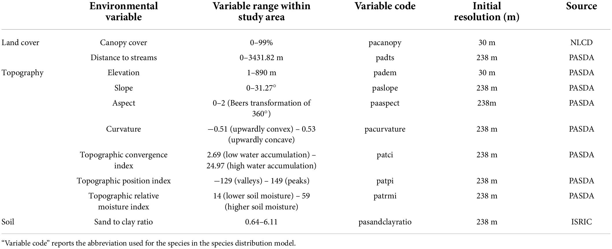
Table 1. Environmental variables used in all species distribution models, the range of values present for each variable, and the initial resolution of the layer.
In preparation for SDM, environmental raster data layers were processed in ArcMap 10.7.1. All rasters were reclassified to have the same cell snaping, mask, and cell size (approximately 238 m2). We generated Elevation, Slope, Aspect, Curvature, Topographic convergence index, Topographic position index, and Topographic relative moisture index (Parker, 1982) layers from the Pennsylvania digital elevation model acquired from PASDA (Pennsylvania Spatial Data Access, 2022). We generated a Distance to streams layer by using the ArcMap Euclidian Distance tool on the streams shapefile acquired from PASDA. The species location points were generated from the TACF dentataBase and we recalculated their coordinates to match with the coordinate system of the environmental layers.
Species distribution modeling
We used ShinyBIOMOD, a graphical interface for the R package “biomod2,” to streamline the SDM process. We defined a geographic region of the state of Pennsylvania and uploaded the species occurrence data and environmental data we previously generated to train and apply the models. As our dataset only contained occurrence records, we generated three pseudo-absence datasets of 290 randomly generated pseudo-absence points in order to run the SDMs. We ran nine different SDMs (summarized in Franklin, 2010) to model C. dentata distribution. These models were ANN, CTA, FDA, GAM, GBM, GLM, MARS, MaxEnt, and RF.
Presence and pseudo-absence points were randomly split into 80% training data and 20% validation data. We ran five replications of all models with each of the three pseudo-absence datasets (totaling 15 replications of each model) to determine C. dentata species distribution and model statistics. Each model replication recorded True Skill Statistic (TSS) and Area-Under-the-Curve (AUC) error evaluation metrics which are commonly used to evaluate model performance (Swets, 1988; Allouche et al., 2006; Fawcett, 2006). Finally, we built ensemble-models of all generated SDMs to evaluate C. dentata distribution as informed by all nine modeling approaches. We generated three different predictions of C. dentata distribution using ensemble modeling outputs. These outputs were predicted probability of presence, binary predictions of presence/absence, and predicted probability of presence by committee agreement of binary individual model outputs. Binary predictions were made by creating a threshold of predicted probability to maximize sensitivity and specificity of the model. This means that a threshold was applied to probability predictions to maximize the true positive rate (sensitivity) and true negative rate (specificity) across the entire range. Pixels with probability values below the threshold were categorized as absences and pixels with probability values above the threshold were categorized as presences.
Results
Comparison of models performance
Accuracy statistics for each species distribution model are summarized in Table 2. These values represent the mean values for AUC (area under the receiver operating characteristics curve) and TSS (True Skill Statistic) between all model replications. AUC values range from 0 to 1 and represents the probability that assigning a predicted suitability value at a random presence point is higher than assigning a predicted suitability value at a random absence point (Fawcett, 2006). Generally, AUC values between 0.6 and 0.7 are interpreted as “fair” models and AUC values between 0.7 and 0.8 are interpreted as “good” models (Swets, 1988; Fawcett, 2006). TSS ranges from −1 to 1, with 0 representing a model that performs no better than random guesses (Allouche et al., 2006). Aside from the random forest models which showed an AUC and TSS value of 1,000, the gradient boosting model and classification tree analysis had the highest AUC and TSS values. AUC and TSS values of 1,000 indicate perfect agreement or fit between errors of sensitivity and specificity (Allouche et al., 2006) and we suspect model overfitting occurred in the random forest model, skewing its results. Artificial neural networks and generalized linear models had the lowest AUC and TSS values.
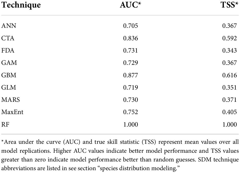
Table 2. Species distribution model performance based on each model’s validation data against the test data.
Environmental variables importance
We generated variable importance measurements for all environmental variables in each SDM technique to identify the most important predictors for C. dentata habitat (Table 3). Sand to clay ratio of the soil was the most frequent top predictor of C. dentata distribution, identified in eight out of nine models. These models identified a positive relationship between sand to clay ratio of the soil and probability of C. dentata presence (indicating higher probability of American chestnut presence in sandier soils). Canopy cover (identified as important in five of eight models) showed a positive relationship with probability of C. dentata presence (indicating higher probability of American chestnut presence in areas of denser canopies). Other important variables included topographic convergence index (three models with a negative relationship) and topographic position index (three models with a positive relationship). The negative relationship with topographic convergence index indicates lower probability of American chestnut presence in areas of higher water accumulation, while the positive relationship with topographic position index indicates a higher probability of American chestnut presence along peaks and ridgeline formations. The artificial neural network model differed the most from other models in identification of variable importance, indicating canopy cover, distance to streams, and elevation as the three most important variables for modeling C. dentata distribution.
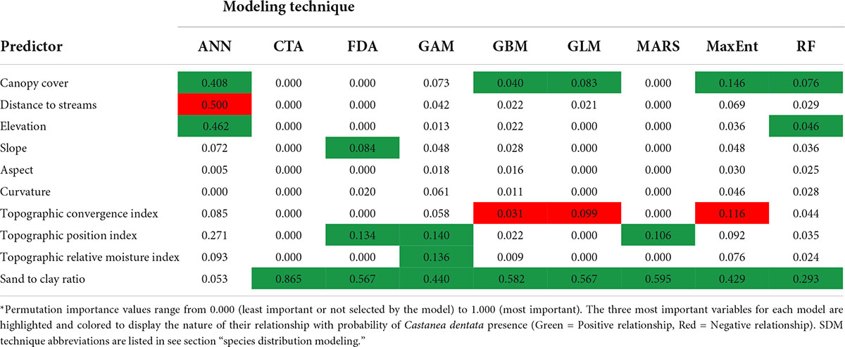
Table 3. Environmental variables used for SDMs and their median permutation importance* for each SDM technique over five replications.
Ensemble model predictions
We generated three maps representing predicted C. dentata species distribution across Pennsylvania through ensemble modeling of all SDMs. The first map (Figure 1A) displays the mean of SDM predictions with the influence of each SDM being weighted by the TSS of that model. This means that all models contributed to determining the suitability of each pixel, but models determined to be more accurate had more influence than models determined to be less accurate. This figure shows higher values of distribution probability in areas such as Pike County in the northeast of the state and along the Spine of Appalachia throughout the center of the state. High areas of C. dentata suitability can also be seen in Allegheny National Forest and along Lake Erie in the northwest of the state.
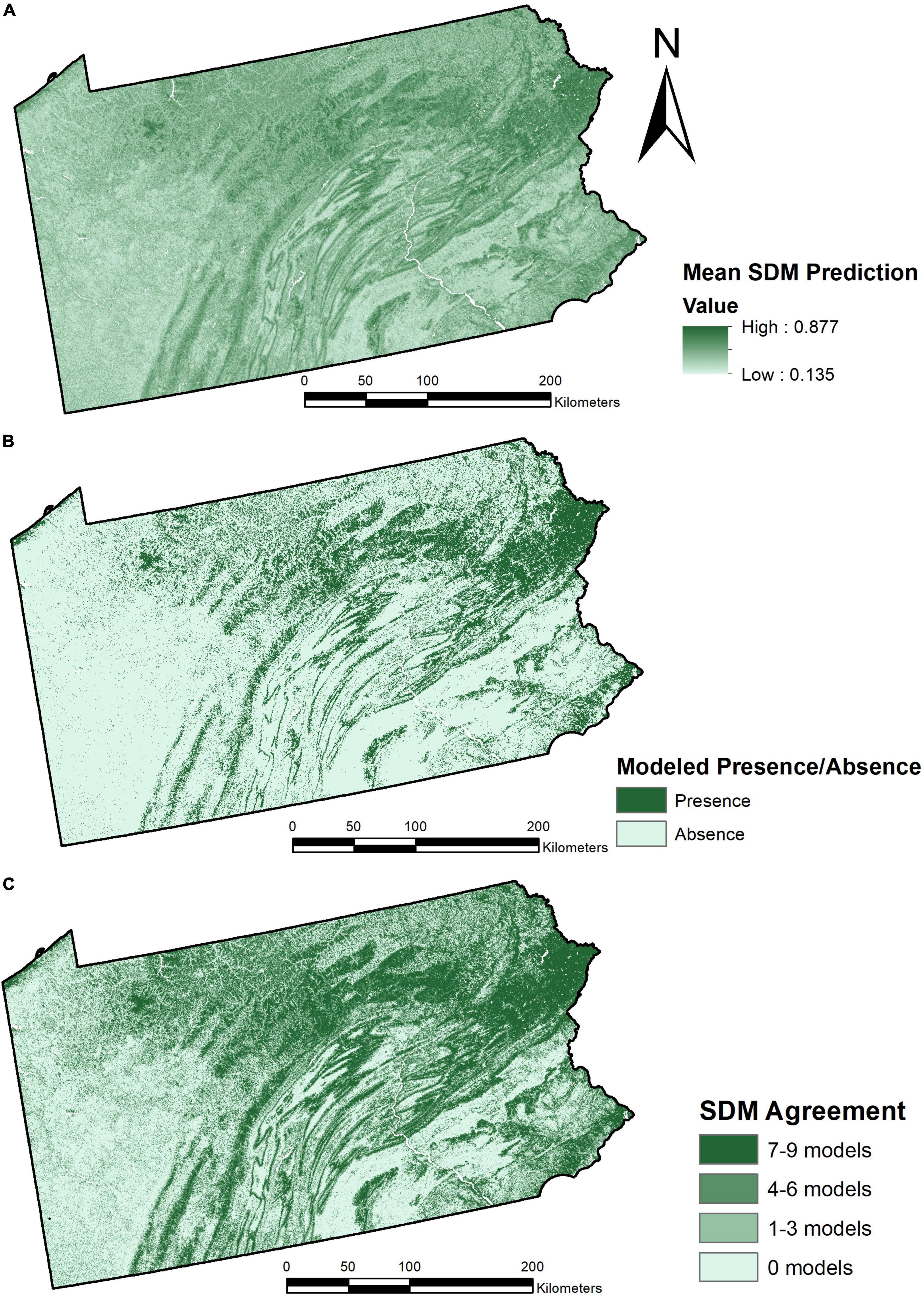
Figure 1. Three panel map showing mean SDM predictions of Castanea dentata distribution weighted by TSS scores of each individual model (A), modeled binary presence/absence of Castanea dentata in Pennsylvania, with a threshold to maximize sensitivity and specificity of the model (B), and SDM techniques committee agreement of species distribution of Castanea dentata (C).
Figure 1B represents a model of binary presence/absence of C. dentata in Pennsylvania based on the combined ensemble model of SDMs. This model defined a suitability threshold in order to maximize the sensitivity and specificity of the prediction. All pixels with suitability values lower than the optimal threshold were defined as absences and all pixels with suitability values higher than the optimal threshold were defined as presences. We determined the optimal threshold to be a value of 0.58, which – when tested with the presence and pseudo-absence points – resulted in 74 true positives, 786 true negatives, 75 false positives, and 23 false negative. According to this binary presence/absence, approximately 16,088 square kilometers of Pennsylvania are considered suitable for C. dentata occupancy.
Finally, we generated a model of predicted spatial distribution of C. dentata in Pennsylvania determined by committee agreement of individual models (Figure 1C). This model was generated by first creating binary presence/absence models for each individual SDM technique, applying a threshold to maximize sensitivity and specificity. Each pixel of the final model is then classified based on how many of the individual SDM techniques classify it as a presence or absence. If 0 models classify it as presence, there is a high consensus of absence. If 1–3 models classify it as presence, there is low consensus of absence. If 4–6 models classify it as presence, there is a low consensus of presence. If 7–9 models classify it as presence, there is high consensus of presence.
Discussion
This study provides insight on the probable spatial distribution of C. dentata across Pennsylvania based on various habitat variables and the effect of different SDM techniques on modeling American chestnut habitat. Most models generally agree with other modeling studies indicating C. dentata suitability is best in high elevation ridgelines with sandy soils and low moisture (Fei et al., 2007; Tulowiecki, 2020). Eight out of the nine models we ran identified sand to clay ratio of the soil as the most important environmental variable, and furthermore indicated a positive relationship between probability of C. dentata presence and sand to clay ratio. Based on this result, we can confidently say that our models are in line with prior studies of C. dentata habitat modeling in addition to knowledge of American chestnut biology. Future modeling studies for C. dentata may consider including additional soil datasets to study this relationship further.
Five out of the nine models identified a canopy cover as one of the three most important environmental variables, and all identified a positive correlation between canopy coverage and probability of C. dentata presence. This finding suggests that American chestnut is more abundant in areas with a more developed overstory. This may be due to the ability of C. dentata to be competitive in lower light environments as it has a history as a generalist species able to thrive in a variety of forested conditions. This result may also reflect the current post-blight niche that smaller diameter surviving C. dentata trees occupy in eastern forests.
Three out of the nine models identified topographic position index as one of the three most important environmental variables and three out of the nine models identified topographic convergence index as one of the three most important variables. These models identified a positive and negative relationship, respectively between these metrics and C. dentata habitat suitability. These findings are supported by the literature and in line with chestnut biology, which indicates that American chestnut is most frequently found on ridgeline and peak topography and in areas of lower water accumulation.
Accuracy statistics such as AUC and TSS allow for model performance evaluation; our high model accuracy values obtained in this study add confidence to our habitat predictions. Most models had AUC values in the 0.7 to 0.8 range, indicating that they performed very well in accurately predicting C. dentata species distribution (Table 2). The artificial neural networks (ANN) model performed the worst out of the nine models with an AUC value of 0.705 and a TSS value of 0.367, suggesting that it is less informative for evaluating C. dentata distribution. Aside from the random forest model (AUC and TSS of 1,000), the best performing model was the gradient boosting model with an AUC value of 0.877 and a TSS value of 0.616. Tulowiecki (2020) also found the gradient boosting model to have the highest AUC of all SDMs when modeling species distribution of C. dentata in western New York. This suggests that gradient boosting models excel in predicting C. dentata distribution based on environmental data and future modeling attempts should include them. An AUC and TSS of 1,000 in the random forest model indicate model overfitting, so these results must be examined further. Because all SDMs utilized randomly generated pseudo-absences points as opposed to collecting true absence data in the field, our models may contain some introduced error. However, the use of multiple pseudo-absence datasets mitigates that error and given the high accuracy metrics of our results and consistency with other studies of C. dentata habitat, we believe that our results are meaningful and valid for habitat prediction.
The lower-performing ANN model also varied the most from other SDM techniques concerning environmental variable importance. This analysis identified canopy cover, distance to streams, and elevation as the three most important environmental variables for determining species distribution of C. dentata. Furthermore, this was the only model that did not identify sand to clay ratio as the most important variable and the only model to identify distance to streams as among the most important. ANN identified distance to streams as having a mean variable importance score of 0.500 – the next highest median variable importance score for distance to streams was MaxEnt with 0.069. For elevation, the random forest model was the only other model to identify it as among the three most important environmental variables. While the ANN model identified the relationship between elevation and probability of C. dentata presence as positive, the relationship between elevation and probability of C. dentata presence identified by the random forest model was more complex, with suitability values varying considerably over the range of elevation values as compared to variation in other models. Even though no other models showed these same variable importance values or relationships, it does make ecological sense that American chestnut would be found at higher elevations further from streams where there would be less soil moisture. Because the ANN model performed the worst based on accuracy statistics and identified different environmental variables as the most important predictors of C. dentata habitat, it may be a less useful technique compared to other SDMs for evaluating suitable American chestnut habitat.
Overall, this study shows a variety of metrics explaining C. dentata species distribution and suggests the usefulness of ensemble modeling of SDMs. By utilizing nine different SDM techniques on the same dataset of species occurrences, pseudo-absences, and environmental variables, this study highlights differences between models that may not appear if models were considered separately. Ensemble modeling also allows for further confidence in results as it allows for direct comparison between different models, enabling the ability to predict whether the same areas are identified as suitable habitat or the relative influence of different environmental variables. For example, eight SDM techniques identified sand to clay ratio as the most important variable in modeling C. dentata distribution and all showed a positive relationship with probability of presence, thus adding weight to this finding. Even though the artificial neural networks model highlighted elevation as a highly important variable for predicting C. dentata distribution in Pennsylvania, the fact that none of the other modeling techniques identified this variable as particularly important suggests that that may be an error or a less significant relationship and we should study the relationship further.
Lastly, we acknowledge that the nature of the collection of C. dentata occurrence records may have introduced some bias into this study as most recorded American chestnut locations are often along trails or roads, where citizen scientists can more readily see the trees. Because we lack accurate data on sampling bias in this dataset, we used randomly generated pseudo-absence points to run the SDMs (Phillips et al., 2009). Additionally, this study is limited by the opacity of some of the modeling outputs. It would be beneficial to be able to explain differences in the mechanics and outputs of each individual modeling approach as it relates to the final ensemble modeling output. This is, however, addressed by the capacity of ensemble models to combine the strengths and weaknesses of the individual SDMs. Future research on C. dentata habitat modeling would benefit from using multi-model approaches that consider a broader set of environmental variables.
Conclusion
This methodology-focused paper presents some of the benefits of using SDM ensemble modeling when studying C. dentata distribution in Pennsylvania. We found that while individual SDM techniques generally picked out similar environmental variables as important predictors of habitat suitability, there was still variation in effect, importance, and accuracy. By combining SDM techniques through ensemble modeling, we can produce distribution maps weighted by accuracy metrics, allowing us to be more confident in the results. This streamlined process of ensemble modeling made possible through “ShinyBIOMOD” and the “biomod2” R package will be useful in assisting conservationists to both find more surviving American chestnut trees and confidently identify areas suitable to reintroduction efforts.
Data availability statement
Publicly available datasets were analyzed in this study. This data can be found here: Environmental variable sources are described in Table 1 of the manuscript coming from https://www.pasda.psu.edu/, https://www.mrlc.gov/data, and https://www.isric.org/explore/isric-soil-data-hub. The dataset of American chestnut locations is not publicly available per TACF data usage agreement.
Author contributions
AH: conceptualization, data collection, methodology, formal data analysis, and writing – original draft. JS: conceptualization, data collection, methodology, formal data analysis, writing – review and editing, and supervision. PK: methodology, writing – review and editing, supervision, and conceptualization. All authors contributed to the article and approved the submitted version.
Funding
This work received funding from Villanova University’s Falvey Memorial Library Scholarship Open Access Reserve (SOAR) Fund.
Acknowledgments
We thank Sara Fitzsimmons at The American Chestnut Foundation (TACF) for providing the input data for this research. We also would like to thank the reviewers of the manuscript for their helpful feedback.
Conflict of interest
The authors declare that the research was conducted in the absence of any commercial or financial relationships that could be construed as a potential conflict of interest.
Publisher’s note
All claims expressed in this article are solely those of the authors and do not necessarily represent those of their affiliated organizations, or those of the publisher, the editors and the reviewers. Any product that may be evaluated in this article, or claim that may be made by its manufacturer, is not guaranteed or endorsed by the publisher.
References
Allouche, O., Tsoar, A., and Kadmon, R. (2006). Assessing the accuracy of species distribution models: Prevalence, kappa and the true skill statistic (TSS). J. Appl. Ecol. 43, 1223–1232. doi: 10.1111/j.1365-2664.2006.01214.x
Barnes, J. C., and Delborne, J. A. (2019). Rethinking restoration targets for American chestnut using species distribution modeling. Biodivers. Conserv. 28, 3199–3220.
Beers, T. W., Dress, P. E., and Wensel, L. C. (1966). Notes and observations: Aspect transformation in site productivity research. J. For. 64, 691–692. doi: 10.1093/jof/64.10.691
Booth, T. H. (2018). Species distribution modelling tools and databases to assist managing forests under climate change. For. Ecol. Manag. 430:1960293. doi: 10.1016/j.foreco.2018.08.019
Collins, R. J., Copenheaver, C. A., Kester, M. E., Barker, E. J., and DeBose, K. G. (2017). American Chestnut: Re-examining the historical attributes of a lost tree. J. For. 116, 68–75. doi: 10.5849/JOF-2016-014
Diamond, S. J., Giles, R. H. Jr., Kirkpatrick, R. L., and Griffin, G. J. (2000). Hard mast production before and after the chestnut blight. Southern J. Appl. For. 24, 196–201. doi: 10.1093/sjaf/24.4.196
Dutech, C., Barres, B., Bridier, J., Robin, C., Milgroom, M. G., and Ravigne, V. (2012). The chestnut blight fungus world tour: Successive introduction events from diverse origins in an invasive plant fungal pathogen. Mol. Ecol. 21, 3931–3946. doi: 10.1111/j.1365-294X.2012.05575.x
Elith, J., and Leathwick, J. R. (2009). Species distribution models: Ecological explanation and prediction across space and time. Annu. Rev. Ecol. Evol. Syst. 2009, 677–697. doi: 10.1146/annurev.ecolsys.110308.120159
Environmental Resources Research Institute (1998). Networked streams of Pennsylvania. Harrisburg, PA: Environmental Resources Research Institute.
Fawcett, T. (2006). An introduction to ROC analysis. Pattern Recogn. Lett. 27, 861–874. doi: 10.1016/j.patrec.2005.10.010
Fei, S., Liang, L., Paillet, F. L., Steiner, K. C., Fang, J., Shen, Z., et al. (2012). Modelling chestnut biogeography for American chestnut restoration: Chestnut biogeography. Divers. Distrib. 18, 754–768. doi: 10.1111/j.1472-4642.2012.00886.x
Fei, S., Schibig, J., and Vance, M. (2007). Spatial habitat modeling of American chestnut at Mammoth Cave National Park. For. Ecol. Manag. 252, 201–207. doi: 10.1016/j.foreco.2007.06.036
Franklin, J. (2010). Mapping species distributions: Spatial inference and prediction. Cambridge: Cambridge University Press.
Homer, C. G., Fry, J. A., and Barnes, C. A. (2012). The National Land Cover Database. The National Land Cover Database (USGS Numbered Series No. 2012–3020; Fact Sheet, Vols. 2012–3020). Reston, VA: U.S. Geological Survey, doi: 10.3133/fs20123020
MacDonald, W. L., Cech, F. C., Luchok, J., and Smith, C. (1978). Proceedings of the American chestnut symposium. Washington, DC: USDA.
Matthews, S. N., Iverson, L. R., Prasad, A. M., Peters, M. P., and Rodewald, P. G. (2011). Modifying climate change habitat models using tree species-specific assessments of model uncertainty and life history-factors. For. Ecol. Manag. 262, 1460–1472.
Milgroom, M. G., Wang, K., Zhou, Y., Lipari, S. E., and Kaneko, S. (1996). Intercontinental population structure of the chestnut blight fungus, Cryphonectria parasitica. Mycologia 88, 179–190. doi: 10.2307/3760921
Noah, P. H., Cagle, N. L., Westbrook, J. L., and Fitzsimmons, S. F. (2021). Identifying resilient restoration targets: Mapping and forecasting habitat suitability for Castanea dentata in Eastern USA under different climate-change scenarios. Clim. Change Ecol. 2:100037. doi: 10.1016/j.ecochg.2021.100037
Nowacki, G. J., and Abrams, M. D. (1992). Community, edaphic, and historical analysis of mixed oak forests of the Ridge and Valley Province, in central Pennsylvania. Can. J. For. Res. 22, 790–800.
Paillet, F. L. (2002). Chestnut: History and ecology of a transformed species. J. Biogeogr. 29, 1517–1530. doi: 10.1046/j.1365-2699.2002.00767.x
Parker, A. J. (1982). The topographic relative moisture index: An approach to soil-moisture assessment in mountain Terrain. Phys. Geogr. 3, 160–168. doi: 10.1080/02723646.1982.10642224
Pennsylvania Spatial Data Access (2022). Available online at: https://www.pasda.psu.edu/ (accessed April 11, 2022).
Phillips, S. J., Dudik, M., Elith, J., Graham, C. H., Lehmann, A., Leathwick, J., et al. (2009). Sample selection bias and presence-only distribution models: Implications for background and pseudo-absence data. Ecol. Appl. 19, 181–197. doi: 10.1890/07-2153.1
Poggio, L., de Sousa, L. M., Batjes, N. H., Heuvelink, G. B. M., Kempen, B., Ribeiro, E., et al. (2021). SoilGrids 2.0: Producing soil information for the globe with quantified spatial uncertainty. Soil 7, 217–240. doi: 10.5194/soil-7-217-2021
Rigling, D., and Prospero, S. (2018). Cryphonectria parasitica, the causal agent of chestnut blight: Invasion history, population biology and disease control. Mol. Plant Pathol. 19, 7–20. doi: 10.1111/mpp.12542
Russell, E. W. B. (1987). Pre-blight distribution of Castanea dentata (Marsh.) Borkh. Bull. Torrey Bot. Club 114, 183–190.
Steiner, K. C., and Carlson, J. E. (2006). “Restoration of American Chestnut to Forest Lands,” in Proceedings of a Conference and Workshop Held May 4-6, 2004 at the North Carolina Arboretum. U.S Department of the Interior, National Park Service, National Capital Region, Center for Urban Ecology, (Asheville, NC). doi: 10.2134/jeq2012.0368
Steiner, K. C., Westbrook, J. W., Hebard, F. V., Georgi, L. L., Powell, W. A., and Fitzsimmons, S. F. (2017). Rescue of American chestnut with extraspecific genes following its destruction by a naturalized pathogen. New For. 48, 317–336. doi: 10.1007/s11056-016-9561-5
Swets, J. A. (1988). Measuring the accuracy of diagnostic systems. Science 240, 1285–1293. doi: 10.1126/science.3287615
TACF (2020). Using Science to Save the American Chestnut Tree [WWW Document]. Asheville, NC: The American Chestnut Foundation.
Thuiller, W., Georges, D., Engler, R., and Breiner, F. (2016). biomod2: Ensemble Platform for Species Distribution Modeling.
Thuiller, W., Lafourcade, B., Engler, R., and Araújo, M. B. (2009). BIOMOD – a platform for ensemble forecasting of species distributions. Ecography 32, 369–373. doi: 10.1111/j.1600-0587.2008.05742.x
Tulowiecki, S. J. (2020). Modeling the historical distribution of American chestnut (Castanea dentata) for potential restoration in western New York State. U.S. For. Ecol. Manag. 462:118003. doi: 10.1016/j.foreco.2020.118003
U.S. Geological Survey (2000). 7.5 minute digital elevation models (DEM) for Pennsylvania (30 meter). Reston, VA: U.S. Geological Survey.
Keywords: American chestnut, species distribution models, ensemble modeling, suitable habitat, restoration
Citation: Henderson AF, Santoro JA and Kremer P (2022) Ensemble modeling for American chestnut distribution: Locating potential restoration sites in Pennsylvania. Front. Ecol. Evol. 10:942766. doi: 10.3389/fevo.2022.942766
Received: 13 May 2022; Accepted: 25 July 2022;
Published: 10 August 2022.
Edited by:
Michael Sears, Clemson University, United StatesReviewed by:
Andrew E. Newhouse, SUNY College of Environmental Science and Forestry, United StatesHill Craddock, University of Tennessee at Chattanooga, United States
Copyright © 2022 Henderson, Santoro and Kremer. This is an open-access article distributed under the terms of the Creative Commons Attribution License (CC BY). The use, distribution or reproduction in other forums is permitted, provided the original author(s) and the copyright owner(s) are credited and that the original publication in this journal is cited, in accordance with accepted academic practice. No use, distribution or reproduction is permitted which does not comply with these terms.
*Correspondence: Alec F. Henderson, YWhlbmRlMTVAdmlsbGFub3ZhLmVkdQ==
†ORCID: Jennifer A. Santoro, orcid.org/0000-0002-7043-7211; Peleg Kremer, orcid.org/0000-0001-6844-5557