 Laurie C. Anderson
 Brooke L. Long-Fox
 Audrey T. Paterson
 Annette S. Engel
95% of researchers rate our articles as excellent or good
Learn more about the work of our research integrity team to safeguard the quality of each article we publish.
Find out more
ORIGINAL RESEARCH article
Front. Ecol. Evol. , 08 July 2022
Sec. Paleoecology
Volume 10 - 2022 | https://doi.org/10.3389/fevo.2022.933486
This article is part of the Research Topic Integrating Conservation Biology and Paleobiology to Manage Biodiversity and Ecosystems in a Changing World View all 22 articles
Comparisons of life and death assemblages are commonly conducted to detect environmental change, including when historical records of live occurrences are unavailable. Most live-dead comparisons focus on assemblage composition, but morphology can also vary in species with environmental variables. Although live-dead morphologic comparisons are less explored, their data could be useful as a proxy in conservation paleobiology. We tested the potential for geometric morphometric data from live-and dead-articulated Stewartia floridana (Bivalvia: Lucinidae) to serve as proxies for seagrass occurrence and stability. The study area is at the northern end of Pine Island in Charlotte Harbor, FL, United States, an estuarine system with substantial seagrass loss in the 20th century and subsequent partial recovery. The area sampled has had relatively stable seagrass occurrences since at least the early 2000s. Live and dead-articulated S. floridana samples were collected from two transects through a patchy seagrass meadow, with sampled sites ranging from bare sand to 100% seagrass cover. Dead-articulated specimens were also collected from three adjacent transects. Live S. floridana shape covaried significantly with seagrass taxonomic composition and percent cover at the time of collection based on two-block partial least squares analysis, although shape differences between seagrass end members (100% Halodule wrightii and 100% Syringodium filiforme) were not significant by multivariate analysis of variance (MANOVA). Instead, specimens from 100% H. wrightii had significantly greater Procrustes variance. Live S. floridana shape data placed in categories describing seagrass stability over 6 years prior to sampling (and reflecting sclerochronologic estimates of maximum longevity) differed significantly based on MANOVA. For live and dead S. floridana from the same transects, shape differed significantly, but allometric trends did not. In addition, patterns of morphologic variation tied to seagrass stability were detected in dead-articulated valve shape. Dead shells from adjacent transects differed significantly in shape and allometric trend from both live and dead specimens collected together. We infer that morphometric differences recorded fine-scale spatial and temporal patterns possibly tied to environmental change. Therefore, geometric morphometrics may be a powerful tool that allows for death assemblages to track seagrass distributions through time prior to systematic monitoring, including in areas under high anthropogenic stress.
Conservation paleobiological approaches that incorporate death assemblages are essential sources of geohistorical data in restoration and conservation studies (e.g., NRC, 2005; Kidwell, 2007, 2013; Dietl and Flessa, 2011; Dietl et al., 2016; Smith et al., 2020), because they can detect community alteration from a variety of timescales, even over a decade or less (e.g., Ferguson, 2008; Poirier et al., 2010; Dietl et al., 2015 and references therein). In addition, live-dead assemblage comparisons can record community reorganization in the recent aftermath of anthropogenic stress (Kidwell, 2007, 2013; Ferguson, 2008; Dietl and Flessa, 2011; Yanes, 2012; Dietl et al., 2015; Dietl and Smith, 2017; Michelson et al., 2018; Tweitmann and Dietl, 2018), invasive species introductions (e.g., Kokesh and Stemann, 2022), and remediation efforts (Gilad et al., 2018; Leonard-Pingel et al., 2019). Death assemblage data can also be used when longer timescales (10–103 years) are needed or when historical records of live occurrences are unavailable to track responses to environmental drivers of ecological change or to disentangle environmental covariates of anthropogenic alteration (e.g., Dietl and Smith, 2017; Gilad et al., 2018; Tweitmann and Dietl, 2018; Leonard-Pingel et al., 2019).
Most live-dead comparative studies document differences in assemblage taxonomic composition, whereas morphologic comparisons, other than size-frequency distributions (e.g., Cummins et al., 1986; Tomašových, 2004; Archuby et al., 2015; Comay et al., 2015; Fuksi et al., 2018), are largely unexplored (although refer to Bush et al., 2002; Krause, 2004). The use of geometric morphometrics as a potential pollution monitoring tool in live-collected mollusks, alone or in combination with other biomarkers, has been increasingly examined, because the techniques are relatively inexpensive (Ambo-Rappe et al., 2008; Harayashiki et al., 2020a,b; Scalici et al., 2020). For example, several studies examine shell shape changes in the limpet Lottia subrugosa relative to pollution gradients and attempt to associate shape changes with metal uptake in shells, enzymatic activity, DNA damage, and lipid peroxidation (e.g., Begliomini et al., 2017; Gouveia et al., 2019; Harayashiki et al., 2020b). Similarly, Ambo-Rappe et al. (2008) described morphologic differences and higher shell asymmetry in Anadara trapezia from seagrass beds exposed to heavy metal contamination, and Scalici et al. (2020) documented geometric morphometric patterns in Mytilus galloprovincialis associated with protein nitration values, polycyclic aromatic hydrocarbon levels, and metal contamination. Although some of these studies used historical live-collected specimens and/or specimens from archeological middens as controls (Harayashiki et al., 2020a for Lottia subrugosa; Márquez et al., 2017 for Buccinanops globulosus), previous studies have primarily focused on live collected specimens from spatially separated polluted and unpolluted areas. Consequently, some environmental variables that could also affect shell shape might not be factored in, including the influence of predators, wave and tide exposure, oxygen levels, temperature, salinity, primary productivity, and variations in water geochemistry affecting calcium carbonate mineral stability (Green et al., 1989; Sokołowski et al., 2008; Neo and Todd, 2011; Comay et al., 2015; Harayashiki et al., 2020b).
Here, we use Stewartia floridana (Bivalvia: Lucinidae) from Charlotte Harbor, FL, United States to (1) test for a geometric morphometric signal of seagrass cover (i.e., seagrass species present and percent of each that covered the site bottom) and for seagrass stability (i.e., number of years that seagrass covered a site prior to sampling) among live-collected shells, (2) test for signal persistence in individuals recovered dead but still articulated from the same sample sites to control for environmental factors that may vary spatially and that could influence morphology, and (3) document the spatial scale of morphological differences by comparing live and dead-articulated shells from the same sites with dead-articulated shells from adjacent sites. Our approach focusing on spatial and temporal resolution in a single seagrass meadow, therefore, circumvents some limitations of previous studies using shell shape as a pollution indicator and instead uses morphology to test a proxy for seagrass coverage both temporally and spatially.
Our findings may be of use for conservation managers, because lucinids play a critical role in seagrass health as the most common chemosymbiotic, infaunal bivalves to inhabit these environmentally sensitive ecosystems worldwide (van der Heide et al., 2012). Seagrasses provide biotic (e.g., primary production, habitat, and nutrient cycling) and abiotic (e.g., sediment stabilization, wave attenuation, and carbon sequestration) ecosystem services to coastal environments nearly worldwide (Duarte, 2002; Orth et al., 2006; Waycott et al., 2009). Because of their environmental sensitivity and ecologic importance, data on seagrass species composition, coverage, and density are commonly used as key ecological components for monitoring ecosystem function (Fourqurean et al., 2002; Orth et al., 2006). For instance, seagrass and other submerged aquatic vegetation (SAV) are extensively used as part of the Comprehensive Everglades Restoration Plan (CERP) to monitor changes in and responses to regional hydrology (USACE, 2019). The Charlotte Harbor Estuary system on the Florida Gulf Coast is immediately north of the Caloosahatchee River Estuary, a drainage pathway for Lake Okeechobee and part of CERP.
Because of the dynamic nature of seagrass distributions due to both natural and anthropogenic factors, a proxy preservable in death assemblages may be able to track seagrass distributions prior to the start of monitoring in a region, as taphonomic inertia (i.e., lag in time it takes for a new community to dilute older communities preserved in death assemblages, Kidwell, 2007) may preserve the signal of seagrass substrates through time. For instance, seagrass monitoring in Charlotte Harbor only began in 1988 (Beever et al., 2011), with estimates of seagrass distributions extending to the 1940s (Harris et al., 1983; Corbett and Madley, 2007). As an inhabitant of intertidal to shallow subtidal seagrass habitats along the western coast of Florida (Fisher and Hand, 1984; Taylor and Glover, 2016, 2021), S. floridana could provide an excellent opportunity to test shell morphometric variation attributed to recent geohistorical and, potentially, paleoenvironmental, changes in seagrass habitat conditions.
The study area encompassed 2,500 m2 directly west of Bokeelia Fishing Pier at Bocilla Island Seaport (N 26.710, W 82.164), at the northern end of Pine Island, FL, on the southern margin of Charlotte Harbor (Figures 1A,B). Charlotte Harbor is the second largest open estuary in Florida, includes three National Wildlife Refuges, and nearly 22,000 ha of state-owned land that were purchased beginning in the 1970s as conservation buffers (Corbett and Madley, 2007). The first Charlotte Harbor Surface Water Improvement and Management Plan was adopted in 1993 and updated in 2000 (Garcia et al., 2020). Although the estuary has been affected in the last century by anthropogenic activities, including phosphate mining, groundwater withdrawal leading to decreased streamflow, and increased nutrient concentrations from wastewater and agricultural runoff (McPherson and Halley, 1996; McPherson et al., 1996; Corbett and Madley, 2007; Tomasko et al., 2020), Charlotte Harbor has not experienced major environmental degradation compared to other Florida estuaries (Garcia et al., 2020). Water clarity remains high (Ott et al., 2006), and the estuary is generally unaffected by nutrient loading or high phytoplankton levels (Greenawalt-Boswell et al., 2006; Julian, 2015; Dixon and Wessel, 2016), although low levels of contamination from heavy metals and polychlorinated biphenyls have been reported (Julian, 2015).
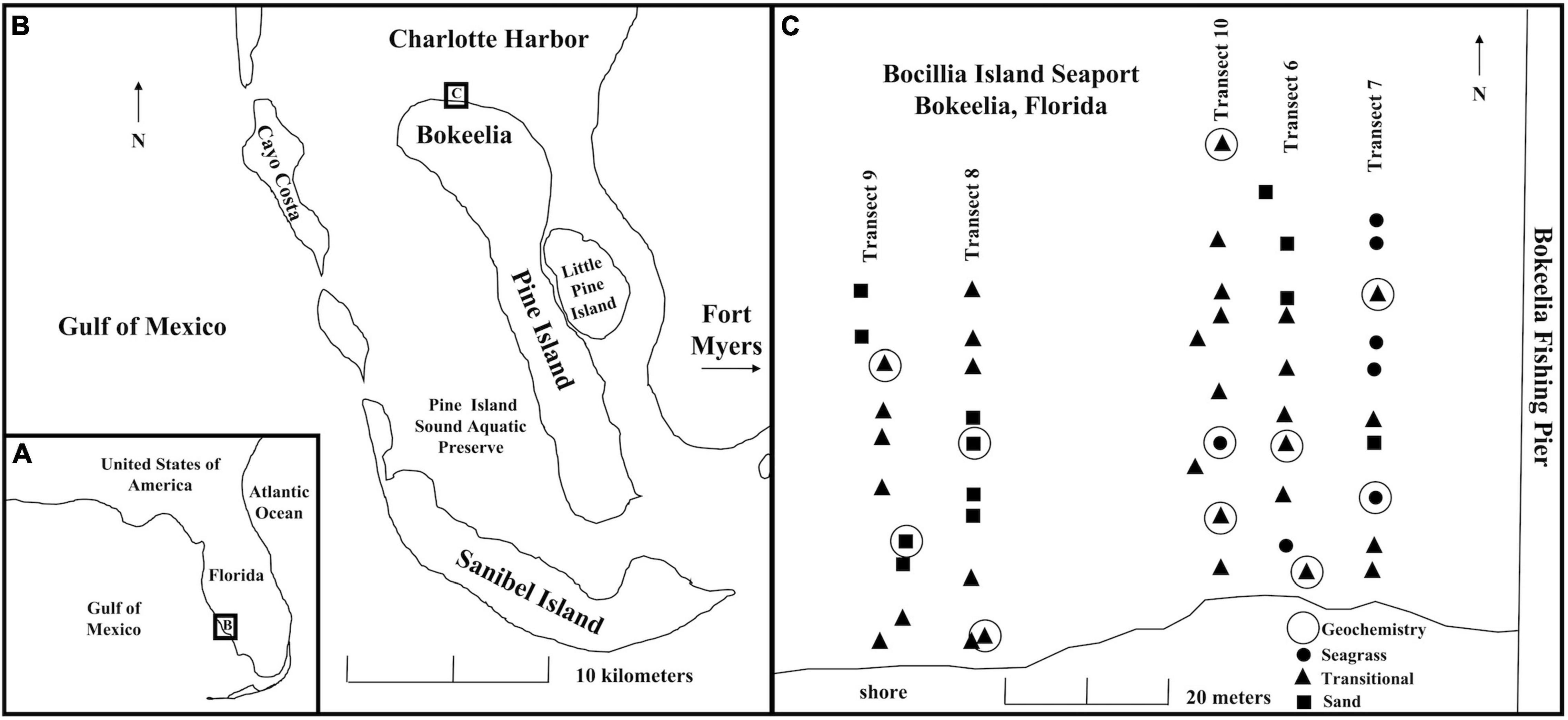
Figure 1. (A) Regional map showing the location of Pine Island relative to Florida. (B) Location of study site on Pine Island indicated by a box labeled with a C. (C) Map of transects and sampled sites in Bokeelia, with symbols reflecting multiyear seagrass stability categories described in Supplementary Table 1 (sand = no seagrass cover; seagrass = complete seagrass cover; transitional = partial seagrass cover). Sites where porewater were collected for geochemistry are indicated by an open circle.
The relatively protected embayment we sampled hosts a narrow strip of discontinuous seagrass (Beever et al., 2011; Yarbro and Carlson, 2016) that has been relatively stable in the past 20 years (Harris et al., 1983; Corbett et al., 2005; Corbett, 2006; Greenawalt-Boswell et al., 2006; Corbett and Madley, 2007; Beever et al., 2011; Brown et al., 2016; Yarbro and Carlson, 2016; Tomasko et al., 2018). Commonly cited causes of seagrass loss in this estuary include human population growth with associated nutrient enrichments in adjacent coastal waters leading to phytoplankton increases and light attenuation, salinity changes due to decreased riverine input, and physical disturbances such as construction of the Intracoastal Waterway and the Sanibel Bridge, as well as propeller scarring (e.g., McPherson et al., 1996; Greenawalt-Boswell et al., 2006; Corbett and Madley, 2007; Beever et al., 2011; Brown et al., 2016; Yarbro and Carlson, 2016; Tomasko et al., 2020). Presently, the estuary is targeted for seagrass protection, but there are no planned restoration efforts (Dixon and Wessel, 2016). Nonetheless, there are goals to restore seagrass cover in CERP to the south of Charlotte Harbor, including the Caloosahatchee Estuary, the Southern Coastal System, and Florida Bay, to maintain ecosystem services by hydrologic modifications that will bring drainage patterns in the Everglades back to a more natural state (USACE, 2019).
In July–August 2014, five 50-m-long sampling transects were established perpendicular to and starting 5 m from the shoreline in the study area (Figure 1C). Each 50-m transect was surveyed at a 5-m interval (i.e., 10 survey points per transect) using a tape and a compass, with sample site locations subsequently recorded with 3-m accuracy at 0.3-m resolution using a Garmin eTrex Vista H with a wide area augmentation system (WAAS)-enabled global positioning system (GPS) receiver.
At each site, a 30-cm diameter area was examined for type and percent of SAV covering the sediment surface prior to water, sediment, and bivalve sample collection (Goemann, 2015; Long, 2016). A mix of seagrass species (Syringodium filiforme, Halodule wrightii, and Thalassia testudinum) had variable coverage at the sampling sites, ranging from 100% seagrass to bare (vegetation-free) siliciclastic sand (Supplementary Table 1). Seagrass cover was tallied in each site in two ways, first by field identification of seagrass species present at the time of collection and their estimated extent of sediment coverage, and second by geospatial analysis of seagrass stability relative to sclerochronologic estimates of S. floridana maximum lifespan in the study area. The latter was carried out to provide a time window encompassing the scale of accretionary growth in S. floridana shells.
To estimate S. floridana lifespan, we measured the stable oxygen isotope composition of carbonate shell material (δ18Oshell) from two live-collected specimens with the largest and thickest (∼1 mm) shells. The specimens were cut into cross-sections along the axis of maximum growth (Supplementary Figure 1) and embedded in fast-setting epoxy resin (J-B KwikWeld) prior to cutting into thick sections using a Buehler Isomet Low Speed saw equipped with a diamond blade. The thick sections were mounted on glass slides and polished with Buehler Silicon Carbide Powder Grit 600. Growth lines along the outer and middle shell layers were examined under a microscope and photographed with a flatbed laser scanner (HP Scanjet 8300) at 4,800 dpi. Carbonate samples were collected by drilling the outer and middle shell layers approximately 0.6 to 1 mm apart along the direction of accretionary growth using a 0.3-mm carbide drill bit (Brasseler H52.11.003 HP Round Carbide). Samples were sent to the University of Arizona’s Environmental Isotope Laboratory where they were mixed with dehydrated phosphoric acid to obtain δ18Oshell measurements in a KIEL-III automated carbonate preparation device connected to a Finnigan MAT 252 gas-ratio mass spectrometer and using the carbonate standards NBS-19 and NBS-18 to define the VPDB (Vienna Pee Dee Belemnite) scale. Analytical precision (1 sigma) for δ18Oshell values was ± 0.01‰. For specimen SDSM 110467, δ18Oshell values ranged from −1.17 to 0.84‰ (Supplementary Figure 2) and for specimen SDSM 110414 from −1.03 to 1.14‰ (Supplementary Figure 3). Using ImageJ (Abràmoff et al., 2004), higher δ18Oshell values (related to colder months) corresponded to opaque bands, and lower δ18Oshell values (i.e., warmer months) corresponded to translucent bands (Supplementary Table 2). By counting coupled growth bands along the axis of maximum growth for all live-collected specimens, we estimated a maximum lifespan of 6 years for S. floridana in the study area.
Using the estimated maximum lifespan, seagrass distributions were geospatially analyzed to document the distribution of seagrass over the last 7 years. Aerial images of Bocilla Island Seaport for 2007, 2009, 2010, 2012, 2013, and 2014 (2008 and 2011 were unavailable) were downloaded from Google Earth and georeferenced to NAD 1983 UTM Zone 17 in ArcGIS (ESRI, 2014). Seagrass and sand area boundaries were digitized into polygon feature classes to produce spatial overlay maps of seagrass and sand through time (Supplementary Figure 4). Three categories were created to classify sample sites for transects 6 and 7: “seagrass” (6 sites) or “sand” (4 sites) for areas with a stable bottom type for over 7 years and a “transitional” category (10 sites) for areas with seagrass cover for a portion of the 7-year interval (Supplementary Table 1). Across all five transects, most of the 50 sample sites were identified as transitional, but seven were categorized as stable seagrass (of any species) and 12 as stable unvegetated sand (Supplementary Table 1). Stability categories did not always match field-observed seagrass coverage estimates because of the spatial resolution of aerial images, seagrass species density, and accuracy of GPS coordinates.
Bivalve sampling from seagrass habitats was permitted under the Florida Fish and Wildlife Conservation Commission (SAL-14-1599-SR). At each site, a 40-cm deep hole was excavated. Coring was not permitted, and the unconsolidated nature of the substrate prevented controlled sampling by depth. Live and dead-articulated S. floridana specimens were collected after sieving sediments through a 3-mm screen. Dead-articulated S. floridana shells were collected from all the transects. However, because of permit-imposed size and count limits, only live specimens ≥10.16 mm in maximum dimension were collected from all the sampling sites in two transects (labeled 6 and 7 on Figure 1C) and a portion of the sampling sites for a third transect (labeled 10 on Figure 1C). Only live specimens from the two full transects were used in our analyses. Stewartia floridana comprised 81% of live and 58% of dead-articulated bivalves collected (Long, 2016). Up to 26 live S. floridana specimens were recovered per site from transects 6 and 7, which resulted in an estimated maximum population density of 867/m3 of sediment. Sites designated as seagrass and transitional stability categories (Supplementary Table 1) had double the number of live S. floridana as the bare sand stability category, which was similar to the distribution of this species in St. Joseph’s Bay, Florida (Fisher and Hand, 1984). All the specimens incorporated into this study are housed at South Dakota School of Mines and Technology’s Museum of Geology (Long, 2016; available in iDigBio Invertebrate Record Set1).
Acquisition of porewater, in addition to overlying ocean water, was essential to evaluate the solubility of aragonite, the mineralogy of S. floridana shells (Kennedy et al., 1969), in the sediment. Porewater was extracted at 11 sites (Figure 1C), including four from transects 6 and 7, from up to 25 cm below the sediment–water interface using a stainless-steel piezometer and a low-flow peristaltic pump (Geotech Environmental Equipment, Inc., Denver, CO, United States) with non-reactive Geotech Silicone tubing (Green-Garcia and Engel, 2012). This sampling depth corresponded to the general burrowing depth of S. floridana in the study area. Water temperature and pH were measured using an Accumet AP115 meter (Fisher Scientific) with a double-junction combination electrode, and conductivity was measured using an Accumet AP75 probe. Once the pumped porewater parameters stabilized, dissolved oxygen (DO) and sulfide concentrations were measured using the CHEMetrics (Calverton, VA, United States) indigo carmine and methylene blue colorimetric methods, respectively, with a V-2000 Multi-Analyte photometer. The pumped porewater was passed through 0.22-μm Millipore Express™ Sterivex polyethersulfone (PES) membrane filter cartridges into separate, prepared HDPE bottles for inorganic anions and cations. Cation bottles were acid-washed with HCl, and field samples were preserved with trace metal grade nitric acid. Alkalinity, as the concentration of total titratable bases but considered to be bicarbonate and carbonate ion species at local pH, was measured from filtered water by titration in the field using 0.1 N sulfuric acid to an endpoint of pH 4.3. Major anion and cation concentrations were measured with Thermo Fisher Dionex ICS2000 ion chromatographs with accuracy of two standard deviations.
Saturation indices (SIs) for aragonite were calculated using thermodynamic models run in PHREEQC Interactive version 3.1.5 (Parkhurst and Appelo, 1999; Supplementary Table 3). The extended form of the Debye-Hückel equation was used to calculate activity coefficients, because ionic strength values were ≤0.1 M. Solubility products (Ksp) were calculated from mass action equations by using programmed ΔG0 values, according to the equation at standard temperature (25°C) and pressure (1 atm) conditions: [ΔG0 = −RT ln Ksp], where R is the gas constant and T is temperature in Kelvin. The ion activity product (IAP) of the solution was compared to Ksp to determine SI, as SI = log (IAP/Ksp). Undersaturated conditions had SI values <0. Because aragonite solubility could be affected by porewater mixing with ocean water in the sediment because of bivalve borrowing activity, mixing models were run with differing contributions of ocean water and sulfidic porewater end-members.
Landmark-based geometric morphometric methods were used to quantify the shell shape and size of live and dead-articulated S. floridana. Only dead specimens ≥10.16 mm in height were used in order to match the minimum size for live specimens (refer to section “Seagrass Cover Estimates and Sample Collection”). Images of left valve interiors were collected using a flatbed scanner (HP Scanjet 8300) at 600 dpi resolution and digitized using tpsDIG2 (Rohlf, 2017). Landmark (LM) placement was based on a simple configuration of seven two-dimensional type 1 and type 2 LMs established by Anderson (2014) to quantify adductor muscle scars, inhalant channel, and pallial line of lucinids (Figure 2). Twenty additional semi-landmarks (SLMs) described the pallial line and the inhalant channel, which is a feature formed by detachment of the pallial line from an elongated anterior adductor muscle. SLMs were obtained by drawing curves from LMs 3 to 4 and from LMs 3 to 5 (Figure 2). In tpsDIG2, each curve was converted to 10 equidistant SLMs with minimized Procrustes distances (Bookstein, 1997; Adams et al., 2015).
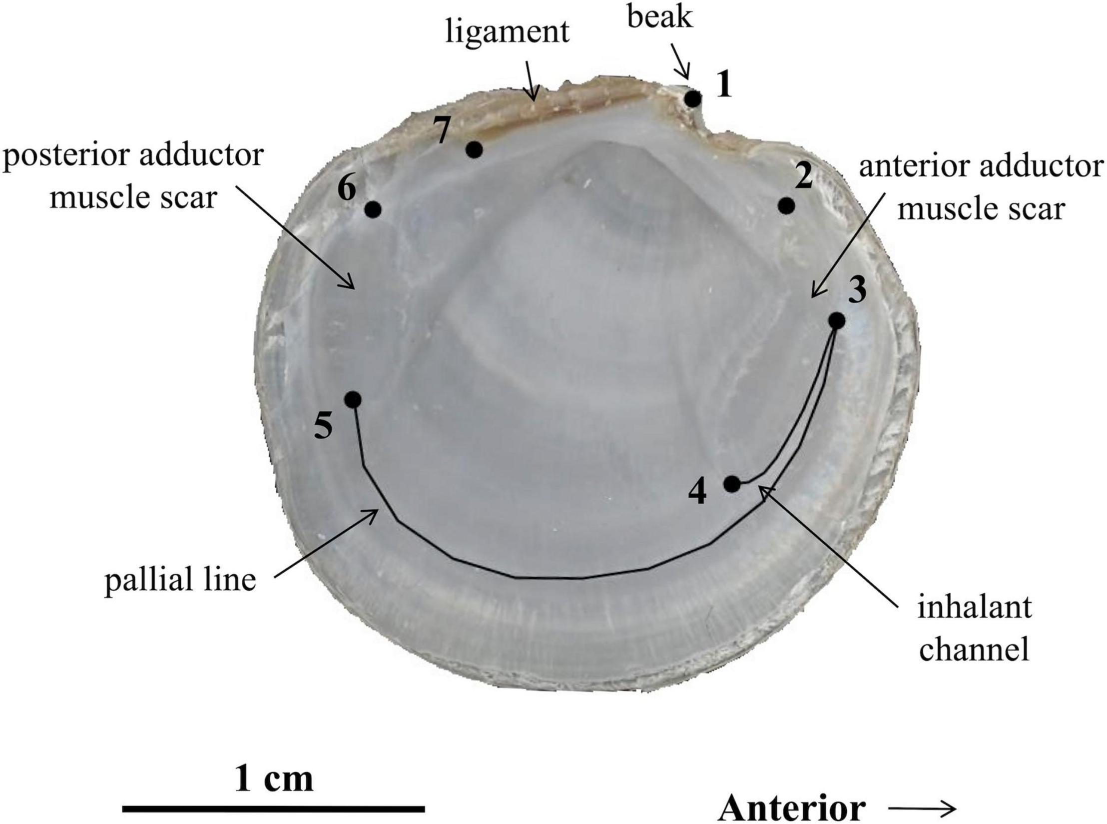
Figure 2. Stewartia floridana left valve showing landmark (LM) and semi-landmark (SLM) curves used in this study. LMs are as follows, clockwise from beak: (1) beak, (2) maximum curvature of the dorsal margin of anterior adductor muscle scar, (3) intersection of the anterior adductor muscle scar and pallial line, (4) maximum curvature of the ventral margin of anterior adductor muscle scar, (5) intersection of the posterior adductor muscle scar and pallial line, (6) maximum curvature of the dorsal margin of posterior adductor muscle scar, and (7) tip of the posterior end of the ligament. SLMs include ten equidistant points, each from LMs 3 to 4 and from LMs 3 to 5, along the illustrated curves.
All geometric morphometric analyses were performed using the geomorph (Adams and Otárola-Castillo, 2013; Adams et al., 2021) and Morpho (Schlager, 2015) packages in R (R Core Development Team, 2020). R code and all associated data files (Supplementary Datasets 1–13) are available in the Supplementary Material. Specimens were placed into four datasets: (1) live-only from transects 6 and 7 (Supplementary Dataset 1.txt), (2) dead-only from transects 6 and 7 (Supplementary Dataset 2.txt), (3) live and dead from transects 6 and 7 (Supplementary Dataset 3.txt), and (4) live from transects 6 and 7, dead from transects 6 and 7, and dead from transects 8, 9, and 10 (Supplementary Dataset 4.txt). Each dataset was superimposed with a Generalized Procrustes Analysis (GPA) to produce Procrustes coordinates and centroid size for each specimen.
Stewartia floridana have uninflated valves (Taylor and Glover, 2021), and all the LMs collected were adjacent to the commissural plane. Therefore, the effects of 2D scanning on LM placement were likely minimal, as previous studies have not indicated substantive differences in results between 2D and 3D geometric morphometric analyses (e.g., Cardini, 2014; Buser et al., 2018; McWhinnie and Parsons, 2019; but refer to Cardini and Chiapelli, 2020 for results using large specimens). Nonetheless, to test for possible differences in inflation that could lead to distortion of 2D configurations, we measured valve inflation for all the specimens using calipers with 0.01 mm resolution and performed a Kruskal–Wallis analysis of variance (or its 2-group equivalent, the Mann–Whitney U test) to test for significant differences in inflation in live specimens across the three seagrass stability categories and between live and dead specimens. In addition, LMs on live specimens were more difficult to visualize and digitize, because their valves were more translucent than those of dead specimens (Figure 3). To assess potential effects of data collection error for the live specimens, we digitized a subset of 20 valves twice, superimposed (using the GPA method described above), and analyzed the results using multivariate analysis of variance (MANOVA). Lastly, we tested for outliers in live-only and live-dead pooled datasets after the GPA by plotting Procrustes distance for each specimen from each dataset’s mean shape and examined outliers for digitization errors.
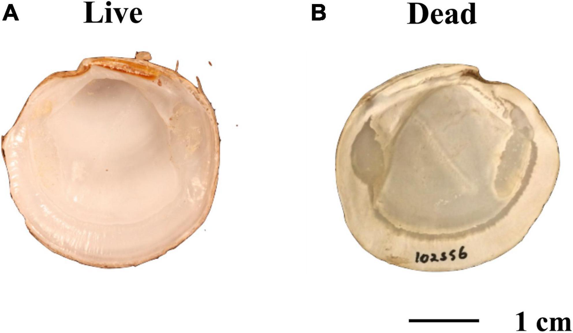
Figure 3. Examples of (A) live and (B) dead specimens showing typical differences in visibility of internal features.
Live and dead-articulated specimens from transects 6 and 7 were tested separately for an association of shape with seagrass coverage (Supplementary Table 1) with a two-block partial least squares (2B-PLS) analysis (Rohlf and Corti, 2000) with 1,000 iterations for significance testing. For the two largest samples of live specimens, which represented 100% cover by H. wrightii and 100% cover by S. filiforme, we also implemented a MANOVA using Procrustes distances in a residual randomization permutation procedure (RRPP) with 1,000 iterations to test for significant differences in shape. Furthermore, morphologic disparity (i.e., an estimate of morphologic dispersion) was calculated as Procrustes variance of shape coordinates for the end-member samples of live specimens, and 1,000 permutations of pairwise differences were used to test for significance. The presence of significant allometry in the live specimen end-member samples, and differences in allometric slopes between these samples, were also tested with multivariate analysis of covariance (MANCOVA).
Live specimen shape was tested for an association with seagrass stability categories (i.e., seagrass, sand, and transitional in Supplementary Table 1) with a MANOVA using Procrustes distances in a RRPP with 1,000 iterations, and p-value adjustment of Holm (1979) for post hoc testing. MANCOVA was conducted to test for a significant allometric trend for the whole dataset and differences in trends for each stability category. Furthermore, morphologic disparity (Procrustes variance) was calculated for seagrass stability categories with 1,000 permutations of pairwise differences to test for significance.
A principal components analysis (PCA) of Procrustes shape coordinates was conducted to visualize separation of stability categories without a priori identification of groups. Canonical variates analysis (CVA) and jackknife cross-validation resampling of Procrustes shape coordinates were carried out to estimate statistical support of stability category assignments. Allometric relationships of stability categories were visualized by plotting regression scores against Log(Centroid Size) and by plotting Log(Centroid Size) against CV1 scores. Thin plate spline (TPS) deformation grids with displacement vectors were used to visualize shape changes along canonical variate (CV) axes.
Two sets of live-dead comparisons were conducted: one 2-group comparison for live and dead specimens collected from transects 6 and 7 and a 3-group comparison for live specimens from transects 6 and 7, dead specimens from transects 6 and 7, and dead specimens from the three adjacent transects (8, 9, and 10). For each comparison, MANOVA using Procrustes distances in a RRPP with 1,000 iterations and p-value adjustment of Holm (1979) for post hoc testing were conducted to test for significant differences among the groups. In addition, PCA was performed to visualize morphologic separation of groups without a priori group identification. Discriminant function analysis (DFA) (for the 2-group comparison) or CVA (for the 3-group comparison) was applied, and a jackknife cross-validation was conducted to test the support of DFA and CVA results. TPS grids with displacement vectors were constructed to examine shape variation along the discriminate function (DF) axis or CV1. As with live-only datasets, pairwise differences in Procrustes variances of shape coordinates were calculated, and 1,000 permutations were used to test for significant differences in morphologic disparity among the groups. Allometry was examined with a MANCOVA for both the 2-group and 3-group comparisons. Allometric trends were visualized by plotting regression scores against Log(Centroid Size) and by plotting Log(Centroid Size) against DFA (2-group) or CV1 (3-group) scores. In addition, for the live and dead specimens from transects 6 and 7, a 6-group CVA that assigned specimens to stability categories was performed with jackknife cross-validation, as well as a MANOVA using Procrustes distances in a RRPP with 1,000 iterations, and p-value adjustment of Holm (1979) for post hoc testing.
Several error tests were conducted prior to in-depth morphometric analyses. First, we found that shell inflation did not differ significantly between the live and dead specimens (Mann–Whitney, p = 0.12). However, when the live specimens were examined alone, those assigned to the sand stability category were significantly different (and were less inflated) from specimens in both the seagrass and transitional categories (Kruskal–Wallis, p = 0.02). As a result, we took this difference into consideration when interpreting TPS grids. Second, although muscle scars were more difficult to image for more translucent, live-collected specimens (Figure 3), MANOVA results indicated that digitization errors in LM placement were minimal (p > 0.05). Lastly, the live-only and live + dead datasets were tested for outliers. For the live-only dataset, three specimens with faint muscle scars fell outside of the upper quartile range and were removed, because their values likely represent measurement error. Reanalysis of both the live-only and live + dead datasets resulted in two outliers detected in the live-only dataset and five in the live + dead dataset. The coordinates digitized for these specimens, however, did not show evidence of error, and these valves were retained in subsequent analyses.
A 2B-PLS analysis of live specimen shape data (n = 137) against seagrass taxonomic composition and coverage determined at the time of collection showed a significant trend (p = 0.028) from 100% cover with H. wrightii to unvegetated to 100% S. filiforme cover (Figure 4A). There was, however, substantial overlap in shape on the x-axis, and the MANOVA results indicated no significant difference in shape (pCover = 0.189; Supplementary Table 4) for the two seagrass end members (which had the largest sample sizes). Differences in Procrustes variance were significant (p = 0.001), and the variance was higher for H. wrightii sites (4.1 × 10⁻³) than for S. filiforme locations (2 × 10⁻³). In addition, the MANCOVA results indicated a significant allometric trend (pLog(CSize) = 0.001) with no significant difference in slopes for the two groups (pInteraction = 0.076; Supplementary Table 4). In summary, there were no consistent differences in shape in the live-collected specimens associated with field-based seagrass cover estimates, although there were significant differences in morphologic variance. For dead-articulated specimens (n = 42) from transects 6 and 7, the 2B-PLS analysis (Figure 4B) was not significant (p = 0.483), although small sample sizes may play a role in reducing statistical power.
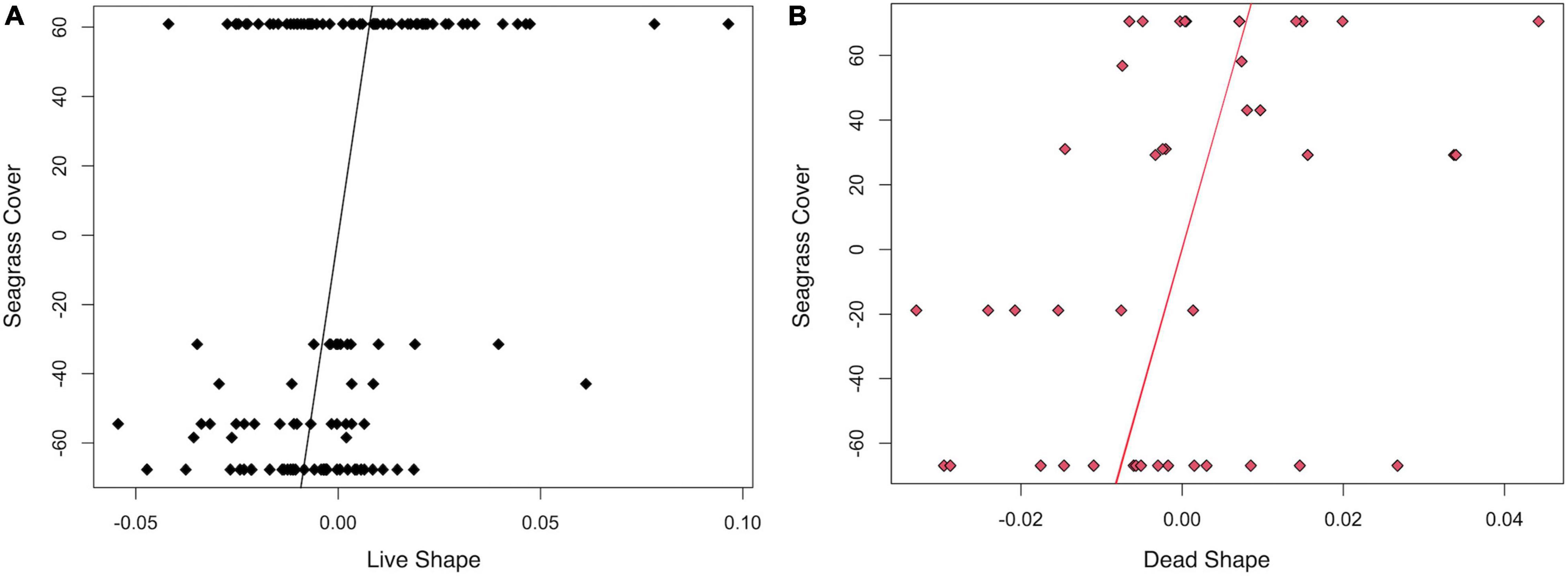
Figure 4. Two-block partial least squares analyses of Procrustes shape (x-axis) by seagrass composition and cover at the time of collection (y-axis) for specimens collected in transects 6 and 7. (A) Live specimens (r-PLS: 0.341, p = 0.028, effect size: 2.1957), with each row representing, from top to bottom, 100% Halodule wrightii, 20% H. wrightii/80% bare sand, 10% H. wrightii/90% bare sand, 100% bare sand, 30% Syringodium filiforme/70% bare sand, and 100% S. filiforme. (B) Dead specimens (r-PLS: 0.383, p = 0.483, effect size: –0.0285), with each row representing, from top to bottom, 100% bare sand, 30% S. filiforme/70% bare sand, 20% H. wrightii/80% bare sand, 6% S. filiforme/54% Thalassia testudinum/40% bare sand, 100% S. filiforme, 50% S. filiforme/50% H. wrightii, and 100% H. wrightii.
Live S. floridana shell shape differed significantly (MANOVA, pStability = 0.001) among the seagrass stability categories, and although shape had a significant allometric trend (MANCOVA, pLog(CSize) = 0.001), the allometric slopes did not differ significantly among the groups (pInteraction = 0.116; Supplementary Table 5 and Supplementary Figure 5). In addition, CV1 scores, which maximized morphological variation among the categories, did not show allometric variation in the groups (Supplementary Figure 6), indicating that group separation was not related to size-dependent shape variation. Furthermore, Procrustes variances among stability categories were not significantly different (Supplementary Table 6), indicating that specimens from the three categories did not differ in their range of morphospace occupation.
The shapes of specimens from seagrass (n = 56) and sand (n = 26) were significantly different based on MANOVA post hoc tests (p = 0.003), as were the shapes of specimens collected from the sand and transitional (n = 55) categories (p = 0.008), although the transitional specimens were not morphologically distinct from the seagrass specimens (p = 0.332; Supplementary Table 7). PCA scores were consistent with these results, with substantial overlap on PC1 and PC2 (which, combined, described about 50% of the variance, Figure 5A). In addition, although the jackknife cross-validation resampling had a relatively low overall classification accuracy of 40% (refer also to Supplementary Table 8), the CVA exhibited greater separation among the stability categories (Figure 5B) than the PCA. On CV1, which accounted for 66.5% of the variance, scores for transitional specimens were intermediate between those of sand and seagrass specimens. CV2 explained the remaining 33.43% of the variation and represented a partial separation of the transitional specimens from the sand and seagrass specimens. Overall, the CVA suggested that morphologic differences among the groups followed a continuum from areas covered by sand in the 6-year window prior to sampling, to sites with seagrass cover for a portion of that time, and to areas continuously seagrass-covered (Figure 5B).
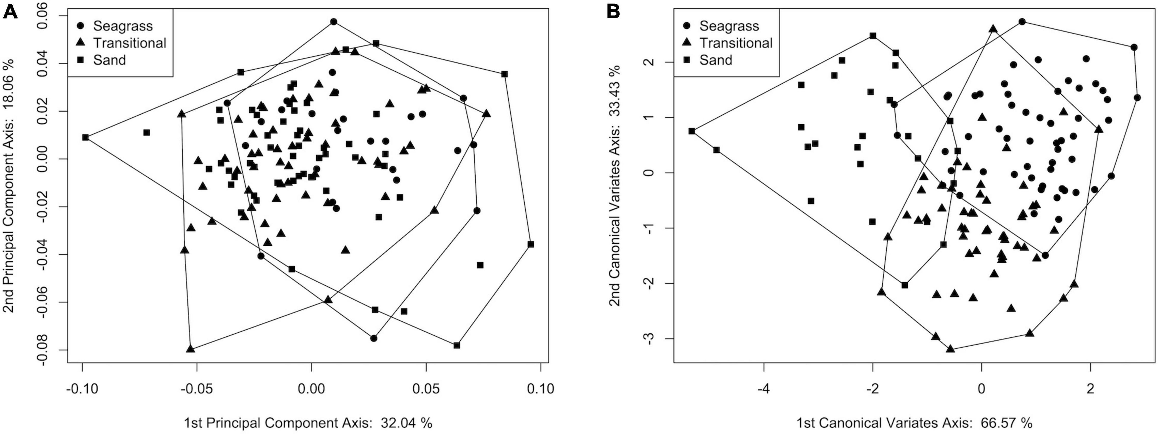
Figure 5. Plots of (A) principal component axis 1 vs. principal component axis 2 scores and (B) canonical variate axis 1 vs. canonical variate axis 2 scores for live S. floridana assigned to stability categories.
A TPS grid depicting variation along CV1 from seagrass to sand specimens indicated (1) an increased inhalant channel length indicated by deformation around LM 3, LM 4, and adjacent SLMs and (2) a wider and more ventrally positioned hinge and beak area (especially deformation around LM 1 and LM 7) that may indicate decreased shell height (Figure 6A). This pattern would not be expected if the cause of morphologic differences were due to lower inflation of specimens from sand-covered sites. In addition, the variation along CV2 represented, from seagrass to transitional specimens, (1) narrowing and slight shortening of the inhalant channel (deformation associated with LM 3, LM 4, and adjacent SLMs) and (2) decreased shell height (deformation associated with LM 1 and LM 7) (Figure 6B).
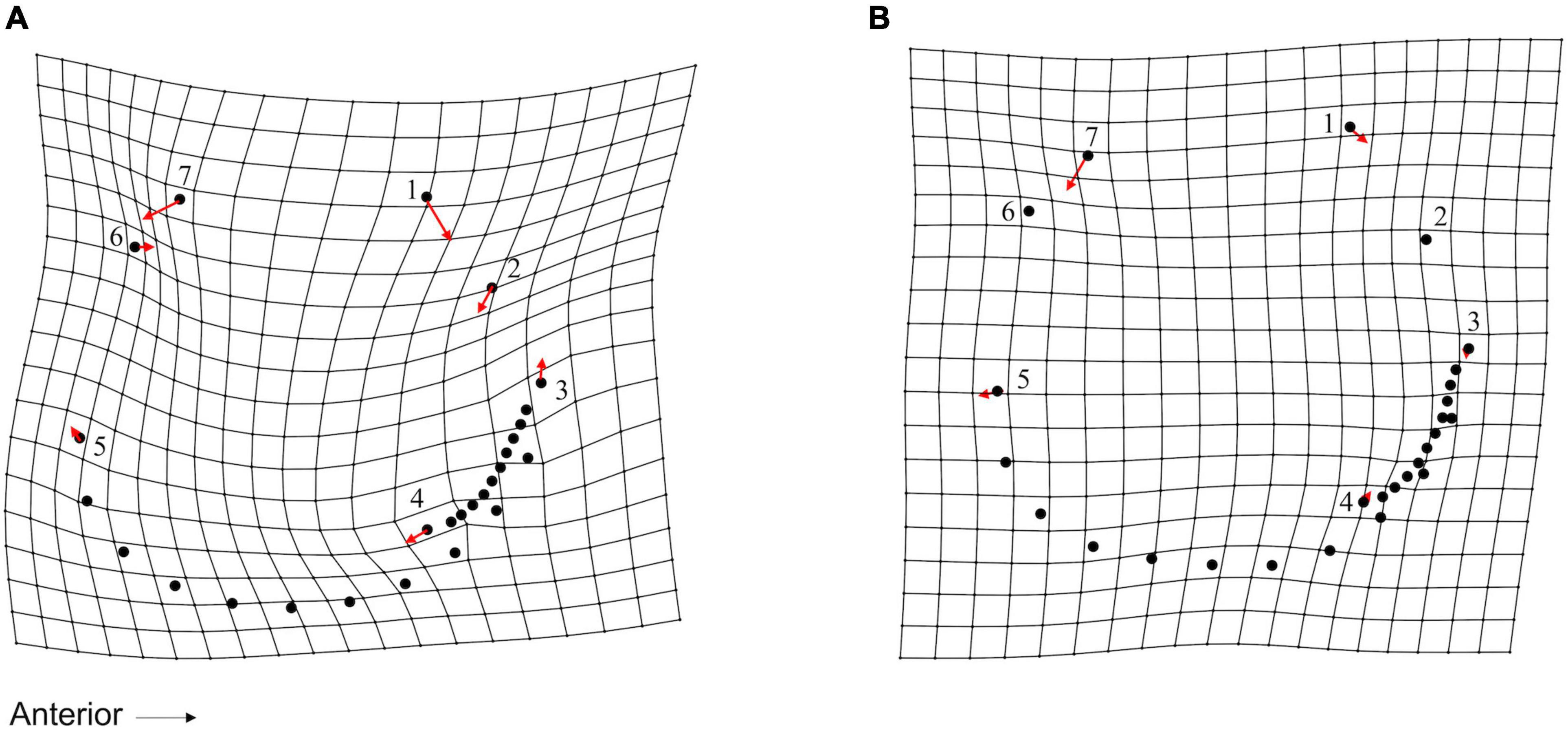
Figure 6. Thin plate spline (TPS) grid, with vectors showing magnitude and direction of LM and SLM deformation, illustrating the shape variation explained along canonical variate axes for live S. floridana in Figure 5B. Each point represents a LM (numbered 1–7, as presented in Figure 2) or an SLM (not numbered) with vectors that illustrate magnitude and direction of deformation on (A) canonical variate axis 1 (CV1) (66.57% of variance) from the maximum (seagrass) to minimum (sand) score values and (B) CV2 (33.43% of variance) from the maximum (seagrass) to minimum (transitional) score values.
In a PCA of live and dead-articulated specimens from transects 6 and 7, the first two axes explained 48.57% of the variance (PC1: 32.09%, PC2: 16.48%), and scores of the dead and live specimens overlapped on both axes (Figure 7A). However, the MANOVA results indicated significant differences in shape between the two groups (pLive/Dead = 0.001; Supplementary Table 9), and the DFA results had high classification accuracy (81.56%), with the live specimens more often correctly assigned than the dead ones (Supplementary Table 10). A TPS grid showing shape change along the DFA axis from live to dead indicated (1) a narrowing of the inhalant channel (deformation associated with LM 3, LM 4, and adjacent SLMs), (2) a posterior shift of beak and hinge areas (deformation associated with LM 1 and LM 7), and (3) an anterodorsal shift of the posterior region (deformation associated with LM 5, LM 6, and adjacent SLMs) (Figure 8). Furthermore, based on MANCOVA, allometry had a significant effect on shape (pLog(CSize) = 0.001), but the live and dead specimens did not have significantly different allometric trends (pInteraction = 0.291; Supplementary Table 9), although shape diverged slightly as size increased (Figure 9A). A plot of DFA vs. Log(Centroid Size) indicated that differences in DFA scores were not related to allometry (Supplementary Figure 7). The live specimens also had greater Procrustes variance (3.5 × 10⁻³) than the dead ones (2.1 × 10⁻³), and the differences were significant (p = 0.004), which can also be seen in the PCA results that showed greater dispersion of the live specimens (Figure 7A).
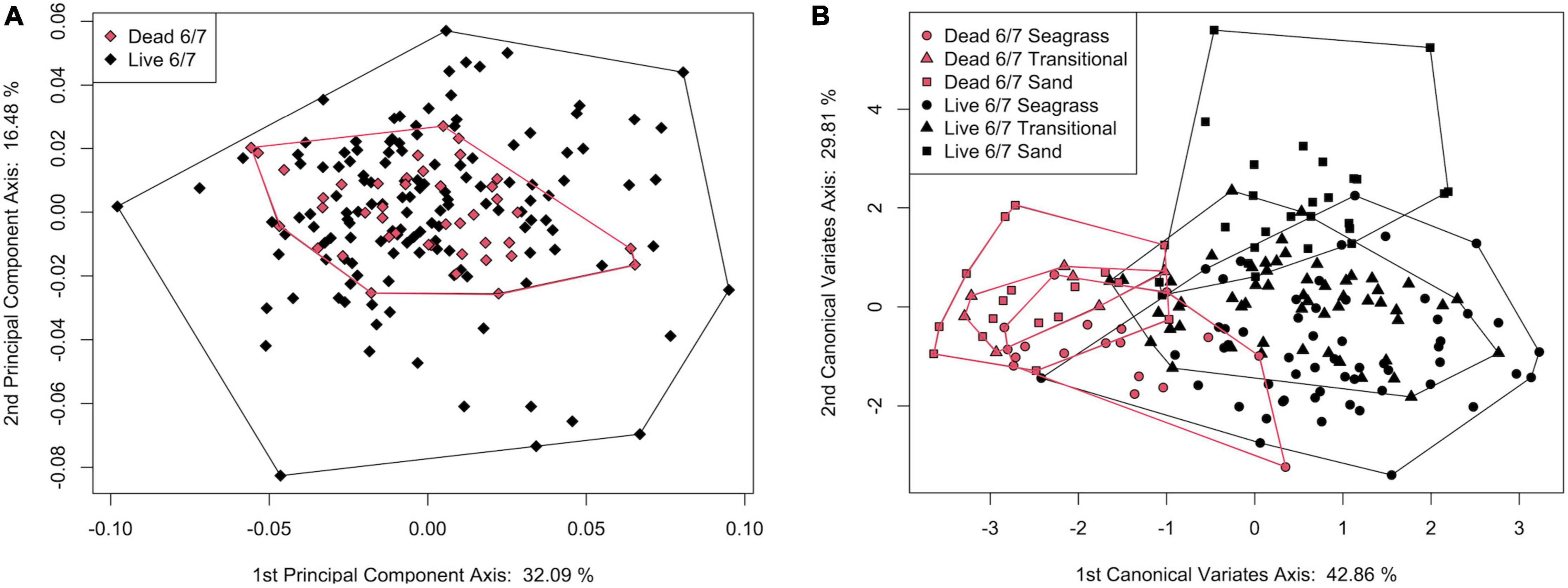
Figure 7. (A) Plot of principal component axis 1 vs. principal component axis 2 for live and dead S. floridana from transects 6 and 7. (B) Plot of canonical variate axis 1 vs. canonical variates axis 2 for live and dead S. floridana specimens from transects 6 and 7 with each assigned to stability categories.
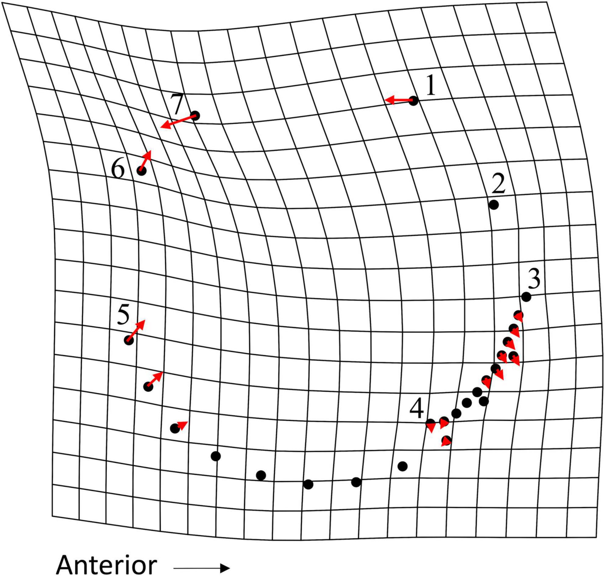
Figure 8. TPS grid, with vectors showing magnitude and direction of LM and SLM deformation, illustrating the shape variation explained along the discriminate function analysis (DFA) axis (refer to Supplementary Figure 7) from maximum (live) to minimum (dead) scores for specimens from transects 6 and 7. Each point represents an LM (numbered 1–7, as presented in Figure 2) or an SLM (not numbered).
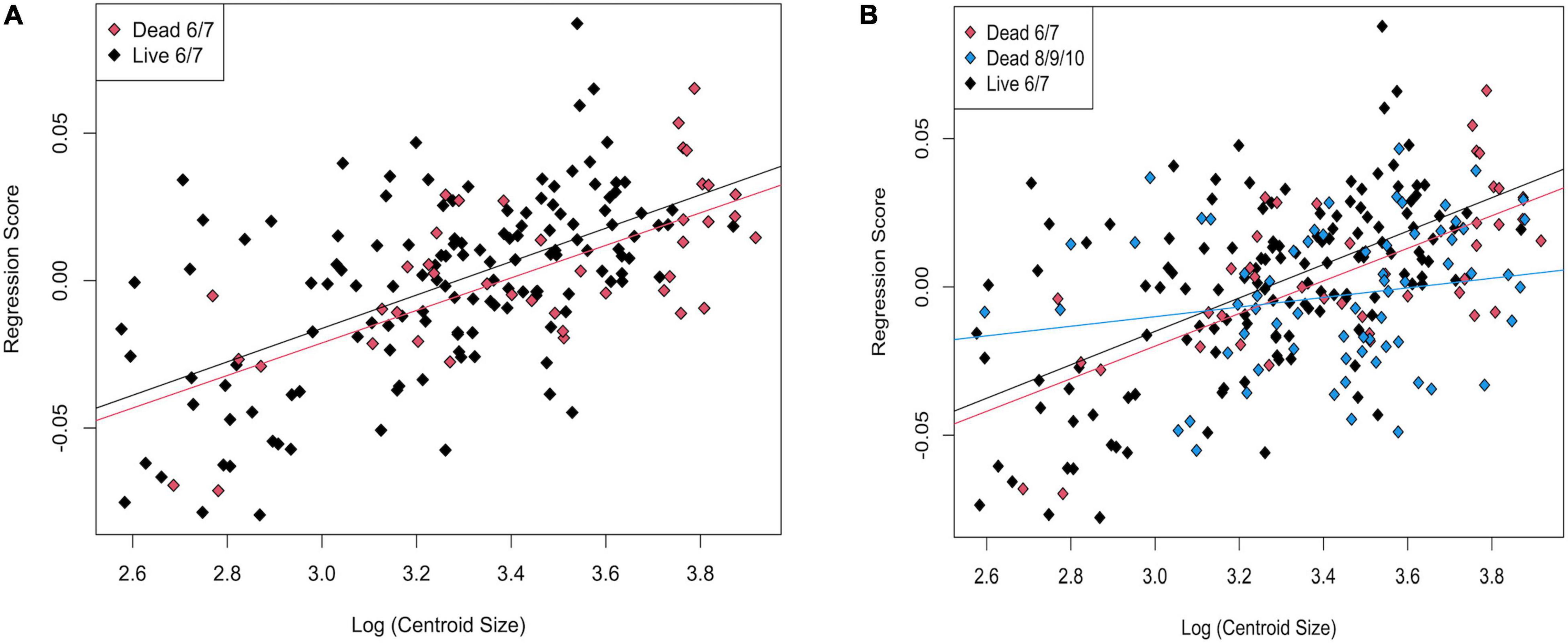
Figure 9. Regression scores vs. Log(Centroid Size) for (A) live and dead specimens from transects 6 and 7; (B) live, dead from transects 6 and 7, and dead from transects 8, 9, and 10.
When both the live and dead specimens from transects 6 and 7 were placed in the stability categories, the MANOVA results indicated significant differences in shape (p = 0.003; Supplementary Table 11), although in the post hoc tests, only 2 pairs of categories were significantly different (live from sand and dead from seagrass and live from seagrass and live from sand, Supplementary Table 12). In a jackknife cross-validation, the classification accuracy was also low (overall ∼33% and ranging from 0 to 42% for individual categories; Supplementary Table 13). In part, the post hoc results may reflect small sample sizes, particularly of the dead groups, as the CVA showed strong separation of live and dead specimens on CV1 (42.86% of variance). However, on CV2 (29.81% of variance), dead specimens had the same order of separation for stability categories as the live ones (which, from negative to positive values, showed a continuum from seagrass to transitional to sand) although with lower variance (Figure 7B).
The addition of dead-articulated specimens from the adjacent transects (8, 9, 10) as a third group (n = 67) produced a PCA with similar variation explained on the first two axes (PC1: 31.51%, PC2 16.48%; Figure 10A). Significant differences in shape among the three groups were found (MANOVA, pLive/Dead = 0.002; Supplementary Table 14), although the post hoc tests indicated that only the comparison of the live with the dead from the adjacent transects was significant (p = 0.006; Supplementary Table 15). Pairwise Procrustes variance comparisons indicated that the live specimens were significantly different from specimens in both dead categories, and that those from the two dead groups were not (Supplementary Table 16). As in the 2-group comparison, the live specimens had higher Procrustes variance. A TPS grid indicated that from live to dead along CV1, the dead specimens had (1) a narrower and shorter inhalant channel (deformation associated with LM 3, LM 4, and adjacent SLMs), (2) reduced shell height, especially posteriorly (deformation associated with LM 1 and LM 7), and (3) a posterior expansion of the posterior portion of the pallial line (SLM deformation ventral to LM 5) (Figure 11). Overall, dead specimens from the same transects were more similar in shape to live specimens than they were to the dead specimens from the adjacent transects.
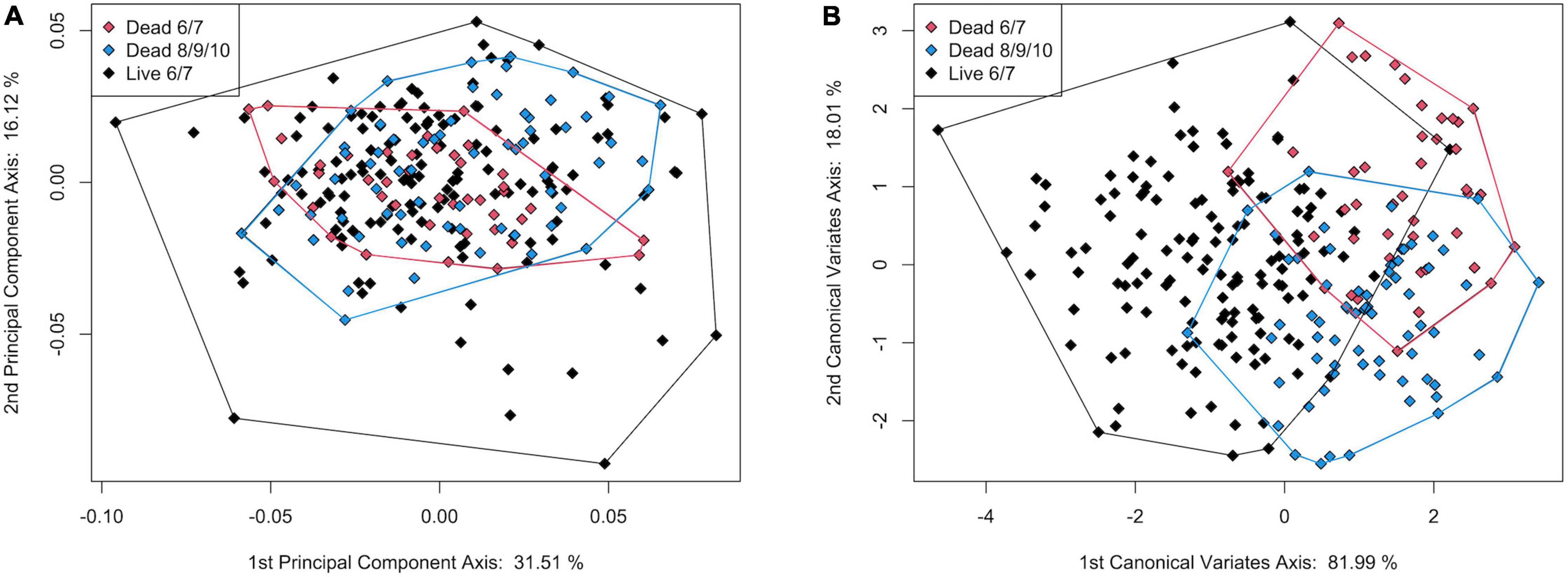
Figure 10. Plot of (A) principal component axis 1 vs. principal component axis 2 and (B) canonical variate axis 1 vs. canonical variate axis 2 for the 3-group comparison of live and dead S. floridana.
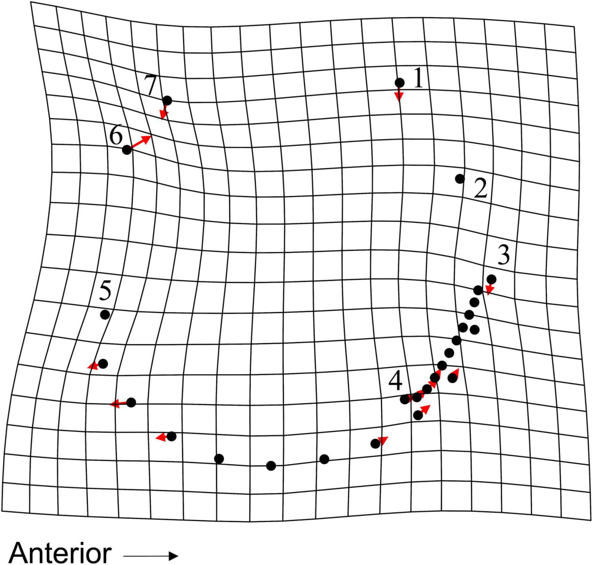
Figure 11. TPS grid, with vectors showing magnitude and direction of LM and SLM deformation, illustrating deformation along CV1 for the 3-group CVA. Deformation shows difference from a live specimen (CV1 = –3.73, CV2 = 0.16) to a dead specimen from transects 8, 9, and 10 (CV1 = 3.4, CV2 = –0.23).
In the CVA, the live and dead specimens separated on CV1 (81.99% of variance), and the dead specimens from transects 6 and 7 separated from those from 8, 9, and 10 on CV2 (18.01% of variance, Figure 10B). The jackknife cross-validation results were relatively low, however, with an overall classification accuracy of 65.04%. The live specimens were correctly assigned 78.10% of the time, but both groups of dead were often incorrectly assigned (45.24% for dead from 6 and 7 and 50.75% for dead from 8, 9, and 10; Supplementary Table 17). Significant allometry (pLog(CSize) = 0.001) was found, and the groups had significantly different allometric trends (pinteraction = 0.002; Supplementary Table 14). This difference was particularly apparent for dead specimens from transects 8, 9, and 10, which had a much shallower allometric slope (Figure 9B). Nonetheless, CV1 scores, which maximize between-group differences, did not have a strong allometric trend (Supplementary Figure 8).
Lucinids are important marine infauna that can provide information about changes in habitat conditions through time, particularly in environmentally sensitive seagrass meadows where they may be the dominant bivalve taxon and form symbiotic relationships with seagrasses (e.g., van der Heide et al., 2012; Gilad et al., 2018; Martin et al., 2020). As relatively deep burrowers (Stanley, 1970), lucinids are potentially protected from physical transport and other post-mortem processes that could impact bivalves living closer to the sediment-water interface. Moreover, adult lucinids are unlikely to move (or be moved) large distances once established (Stanley, 1970). Given this potential for fine-scale spatial resolution in live and dead lucinid distributions, we used S. floridana, in a single seagrass meadow, to (1) test for a geometric morphometric signal of seagrass cover and for seagrass stability among live-collected shells, (2) test for signal persistence in dead-articulated individuals from the same sample sites to control for environmental factors that may vary spatially and that could influence morphology, and (3) document the spatial scale of morphologic differences by comparing live and dead-articulated shells from the same sites with dead-articulated shells from adjacent sites.
Seagrasses are important ecosystem engineers of coastal biomes worldwide, host some of the most productive ecosystems on earth, play a critical role in carbon sequestration (Mcleod et al., 2011), and serve as sentinel taxa for ecosystem health (Orth et al., 2006; Waycott et al., 2009; Brown et al., 2016). Seagrass beds are highly impacted by anthropogenic drivers of ecologic change (Halpern et al., 2008), with losses accelerating globally in the latter half of the 20th century (Orth et al., 2006; Waycott et al., 2009). Monitoring seagrass beds can help to understand and mitigate this loss, but systematic programs only began within the last few decades, thereby post-dating the start of anthropogenic impacts to many estuarine systems (Brewster-Wingard and Ishman, 1999; Orth et al., 2006; Cullen-Unsworth and Unsworth, 2016). As baselines shift, it becomes difficult to reconstruct pre-impact conditions, determine original causes for loss, and track historical distributions of seagrasses and other SAV (Fourqurean and Robblee, 1999; Fourqurean et al., 2003). Furthermore, even with restoration and recolonization, the original structure of the seagrass bed ecosystem may not be recovered (Gilad et al., 2018). Therefore, conservation paleobiology approaches have a great potential to track changes in seagrass habitats and characterize parameters that could define a return of ecosystem function.
Our results indicated that S. floridana shape could serve as a proxy for seagrass coverage, as the morphology of live-collected specimens varied significantly with seagrass stability but not necessarily seagrass cover at the time of collection. The shape of live specimens recovered from bare sand differed significantly (e.g., having generally more elongate valves with longer inhalant channels) from specimens recovered from sites covered in seagrass during all or part of the 6 years prior to collection. In contrast, we did not find a significant difference in the mean shape of live specimens from sites covered by specific seagrass species. Instead, specimens from 100% H. wrightii had a significantly greater shape variance, which could be related to more ephemeral occurrences of Halodule spp. in south Florida, as this is an early successional taxon that can tolerate higher nutrient availability and more variable salinities than other seagrass taxa common in the area (Fourqurean et al., 2002, 2003; Fourqurean and Rutten, 2004; Greenawalt-Boswell et al., 2006; Orth et al., 2006; Ferguson, 2008). Our results also indicated that although live and dead specimens from the same transects differed significantly in shape, the morphologic transition from stable seagrass to stable sand in live S. floridana can also be recovered in the dead specimens. Furthermore, the shapes of live and dead S. floridana from the same transects were more similar to each other than to those of dead specimens from the adjacent transects.
Because S. floridana lack hinge teeth, their shells may be prone to disarticulation once the ligament decays, so dead-articulated shells could represent both minimal post-mortem transport and time averaging. Although we do not know the time of death of the dead-articulated S. floridana specimens, the amount of time averaging represented by these specimens, or whether either time of death or time-averaging was different across transects, we initially predicted that the morphology of live and dead-articulated S. floridana would substantially overlap, as this pattern is reported in other taxa even in cases where fossil specimens were incorporated into analyses. For instance, using a geometric morphometric approach, Bush et al. (2002) did not find differences in morphologic variability between live-collected Mercenaria and Pleistocene congeners, although mean morphology did change in association with paleocommunity transitions. Similarly, Krause (2004) found comparable mean shape and shape variability in live and dead-articulated Terebratalia transversa. Our results, instead, indicated significant differences in mean shape and shape variability in live and dead-articulated shells collected from the same sites, even though time averaging and post-mortem transport were minimized using only dead-articulated shells in a species with a moderate life span (up to 6 years) and a relatively deep burial depth (up to 20 cm; Fisher and Hand, 1984). We attribute these differences primarily to a morphologic response of S. floridana to spatially and temporally changing substrate conditions, specifically seagrass stability.
Allometric trends could explain some live-dead shape differences observed, but the role of allometry in among-group shape separation is complicated. Our analyses suggested no significant differences in allometric slopes for live specimens among stability categories or for the 2-group comparison of live and dead-articulated shells from the same transects. There were, however, significant differences in the 3-group comparison that included dead-articulated specimens from different transects. In both the 2-group and 3-group analyses, the slopes of live and dead specimens from the same transects diverged as size increased, so these specimens had greater morphological similarity at smaller sizes. In the adjacent transects, dead individuals had a shallower allometric slope that intersected the other two trends, so smaller and larger specimens diverged in shape from the live and dead specimens from transects 6 and 7. Moreover, we found that the live specimens occupied a larger morphospace that included morphologies outside the range observed in the dead ones, which would not be expected if allometry alone explained the shape differences.
The post-mortem transition from translucent to opaque shells in S. floridana is quite dramatic, and muscle scars on dead, opaque valves were much easier to observe and digitize. For some live specimens, adductor scar positions at earlier growth stages on the accretionary valve were visible above the dorsal margins of adductor scars (we digitized the latest formed positions of the adductor scars in these instances). Such differences could lead to greater variability in shape for live than for dead specimens, which we observed, if that variability is caused by digitization error. However, the MANOVA results indicated that changes in shell translucency did not affect the accuracy of LM placement. In addition, we would not predict that such error would lead to differences in mean shape between live and dead specimens, as we found.
Similar opacity differences between live and dead pteropods are well-documented and linked to aragonite dissolution, which is considered an indicator of ocean acidification (e.g., Bednaršek et al., 2019; Oakes and Sessa, 2020). In pteropods, transition from transparent to milky white can occur within days after death and is associated with soft tissue oxidation before shells sink below the aragonite saturation zone (Oakes et al., 2019). In fact, Oakes et al. (2019) considered post-mortem oxidation of internal organic matter to have a greater impact on shell dissolution than seawater saturation state. Our thermodynamic modeling indicated that fluids with higher pH values were supersaturated with respect to aragonite (Supplementary Figure 9), but one porewater sample from a 100% seagrass site (50% H. wrightii and 50% S. filiforme) was undersaturated with respect to aragonite. From mixing models, porewater could become undersaturated with respect to aragonite if mixed with less than 25% ocean water (Supplementary Figure 9), which could result from processes such as bioturbation (McPherson et al., 1996), or changes in tidal pumping, wave-base circulation, and turbulent sedimentation events. Therefore, potential soft tissue decay and aragonite dissolution in the sediment could explain translucent to opaque alteration for dead shells, but we infer that incipient dissolution is not likely to affect the location, shape, or size of muscle scars in dead shells.
Muscle scars in bivalves have a characteristic microstructure (myostracum; Stenzel, 1963; Kennedy et al., 1969; Lee et al., 2011) composed of aragonite prisms oriented perpendicular to the valve surface (Suzuki and Nagasawa, 2013). Because shells grow by accretion, inner shell layers are laid over the myostracum from earlier formed portions of the valve (Kennedy et al., 1969; Garcia-March et al., 2011; Lee et al., 2011; Nishida et al., 2011). If we assume that dissolution altered the valves from their outer surfaces inward, then we might predict that earlier precipitated myostracal layers would become exposed on dead shells, thereby lengthening adductor scars by shifting LMs that define their dorsal margins in a dorsal direction. Our TPS results, however, indicated an opposite trend in both the 2-group and 3-group live-dead comparisons, except possibly for LM 6 at the dorsal maximum of the posterior adductor scar, which generally is more ventrally positioned in live specimens. Furthermore, other morphologic differences between the live and dead specimens, including changes in shell height (e.g., live were higher), position of the beak and hinge, and the intersection of the pallial line and posterior adductor scar, cannot be related to exposure of myostracum by dissolution. In addition, shape differed between dead specimens from transects 6 and 7 and those from the adjacent transects, which we would not predict if taphonomic alteration is a factor in LM placement. Finally, taphonomic alteration should be greatest for smaller shells (Cummins et al., 1986), which have a larger relative surface area. However, we found that allometric trends of live and dead specimens from the same transects overlapped at small valve sizes and diverged as size increased.
Because live S. floridana shell shape changed on a continuum from stable seagrass to stable bare sand, which also was recorded in dead-articulated specimen shape from the same transects, and because of differences in allometric trends between live and dead specimens from different sampling transects, shell accretionary growth and shape are likely affected by local spatial and temporal environmental changes. The presence and stability of seagrass, as well as overall porewater and seawater chemistry, could be important conditions that influence lucinid growth and respiration. Seagrasses release oxygen from their roots into surrounding sediments (Borum et al., 2007; van der Heide et al., 2012), and the availability of oxygenated water while living in seagrass-stabilized sediment may be higher than in bare sand, which may influence the shape of the inhalant channel as well as overall shell shape. In lucinids, oxygenated ocean water is brought in through a constructed inhalant tube and used by both the lucinid host and chemosymbiotic sulfur-oxidizing bacteria in gill bacteriocytes (Taylor and Glover, 2006). Fisher and Hand (1984), however, did not observe tubes long enough to reach oxygenated ocean water in S. floridana, so the release of oxygen by seagrass rhizomes is likely an important source of oxygen in this species. This may also explain the higher abundance of this taxon in seagrass than in sand in this study, as well as in Fisher and Hand (1984).
Reponses to environmental change, coupled with time averaging that exceeds the scale of that change, likely explains the live-dead shape mismatch observed in S. floridana. Therefore, the morphometric signals we observed have the potential to be used as a proxy to track fine-scale environmental conditions occurring within and across seagrass beds. Although the seagrass beds in Charlotte Harbor have remained stable on an estuary-wide scale for about 20 years, small-scale spatial changes (i.e., at the transect scale) are apparent from our study (Supplementary Table 1 and Supplementary Figure 4) and temporal changes in Halodule and Thalassia percent cover are documented (Greenawalt-Boswell et al., 2006). Use of the S. floridana morphometric proxy could allow for historic distributions of stable seagrass beds in the region to be identified and verified. Furthermore, the proxy may serve to test whether restored seagrass beds have similar environmental conditions and possible ecosystem functions to their predecessors. In these ways, this proxy can contribute to the use of seagrasses as indicator species in areas undergoing ecosystem monitoring and restoration (e.g., USACE, 2019).
In recent years, morphology-based metrics for biomonitoring have been increasingly implemented in conservation (paleo)biology studies. Morphometric differences documented in mollusk shells from prior research, however, are complicated by known morphologic responses to a myriad of environmental factors that vary spatially and temporally. We controlled for these factors in a conservation paleobiology approach, by comparing live and dead-articulated specimens of S. floridana from the same sample sites with dead-articulated specimens from the adjacent sites. We found that although the live and dead specimens differ in shape, the shape trends observed in live S. floridana associated with multiyear seagrass stability could also be detected in dead-articulated specimens from the same sites. Furthermore, the morphologic comparisons of live and dead specimens from the same transects with dead-articulated specimens from the adjacent transects indicated fine-scale spatial and temporal shape variation. Geometric morphometrics of death assemblages, therefore, may provide powerful tools for conservation managers to monitor the historical distribution of seagrass habitats and their ecosystem function through time.
The original data for this study are included in the Supplementary Material, further inquiries can be directed to the corresponding author.
BL-F and LA conceived the idea for this project. BL-F, LA, AE, and AP planned and conducted the field work. BL-F contributed in morphometric analyses and constructed the figures and tables. AE and AP provided the geochemical data, analyses, text, figures, and tables. AP conducted field identifications of seagrass species coverage. BL-F and LA collaborated on initial drafts of the text, with additions from AE. All authors contributed to revisions of the manuscript and approved the final version.
This research was supported by the National Science Foundation DEB-1342721 (LA), NSF-DEB-1342785 (AE), and NSF-DEB-1342763 (B. Campbell).
The authors declare that the research was conducted in the absence of any commercial or financial relationships that could be construed as a potential conflict of interest.
All claims expressed in this article are solely those of the authors and do not necessarily represent those of their affiliated organizations, or those of the publisher, the editors and the reviewers. Any product that may be evaluated in this article, or claim that may be made by its manufacturer, is not guaranteed or endorsed by the publisher.
Sampling was permitted under the Florida Fish and Wildlife Conservation Commission (SAL-14-1599-SR). Permission to access and conduct research at the Bokeelia Fishing Pier was granted by the landowners, and field work assistance was provided by A. Goemann, T. W. Doty, B. J. Campbell, and S. J. Lim. Thanks to David Dettman, University of Arizona’s Environmental Isotope Laboratory, for the stable isotope analyses. Thank you also to the two reviewers and co-editors of this volume, particularly GW, for suggestions that improved the manuscript.
The Supplementary Material for this article can be found online at: https://www.frontiersin.org/articles/10.3389/fevo.2022.933486/full#supplementary-material
Abràmoff, M. D., Magalhães, P. J., and Ram, S. J. (2004). Image processing with imageJ. Biophotonics Int. 11, 36–42.
Adams, D. C., and Otárola-Castillo, E. (2013). geomorph: an R package for the collection and analysis of geometric morphometric shape data. Methods Ecol. Evol. 4, 393–399. doi: 10.1111/2041-210X.12035
Adams, D. C., Collyer, M. L., and Sherratt, E. (2015). geomorph: Software for Geometric Morphometric Analyses: R Package Version 3.0. Available online at: http://cran.r-project.org/web/packages/geomorph/index.html (accessed April 24, 2022).
Adams, D. C., Collyer, M. L., Kaliontzopoulou, A., and Baken, E. K. (2021). Geomorph: Software for Geometric Morphometric Analyses. R package Version 4.0. Available online at: https://cran.r-project.org/package=geomorph (accessed April 24, 2022).
Ambo-Rappe, R., Lajus, D. L., and Schreider, M. J. (2008). Higher fluctuating asymmetry: indication of stress on Anadara trapezia associated with contaminated seagrass. Environ. Bioindic. 3, 3–10. doi: 10.1080/15555270701779460
Anderson, L. C. (2014). “Relationship of internal shell features to chemosymbiosis, life position, and geometric constraints within the Lucinidae (Bivalvia),” in Experimental Approaches to Understanding Fossil Organisms, eds S. I. Hembree, B. F. Platt, and J. J. Smith (Dordrecht: Springer Netherlands), 49–72. doi: 10.1007/978-94-017-8721-5_3
Archuby, F. M., Adami, M., Martinelli, J. C., Gordillo, S., Boretto, G. M., and Malvé, M. E. (2015). Regional-scale compositional and size fidelity of rocky intertidal communities from the Patagonian Atlantic coast. Palaios 30, 627–643. doi: 10.2110/palo.2014.054
Bednaršek, N., Feely, R. A., Howes, E. L., Hunt, B. P. V., Kessouri, F., León, P., et al. (2019). Systematic review and meta-analysis toward synthesis of thresholds of ocean acidification impacts on calcifying pteropods and interactions with warming. Front. Mar. Sci. 6:227. doi: 10.3389/fmars.2019.00227
Beever, J. III, Gray, W., Beever, L. B., and Cobb, D. (2011). A Watershed Analysis of Permitted Coastal Wetland Impacts and Mitigation Methods within the Charlotte Harbor National Estuary Program Study Area. Fort Myers, FL: Southwest Florida Regional Planning Council.
Begliomini, F. N., Maciel, D. C., De Almeida, S. M., Abessa, D. M., Maranho, L. A., Pereira, C. S., et al. (2017). Shell alterations in limpets as putative biomarkers for multi-impacted coastal areas. Environ. Pollut. 226, 494–503. doi: 10.1016/j.envpol.2017.04.045
Bookstein, F. J. (1997). Landmark methods for forms without landmarks: morphometrics of group differences in outline shape. Med. Image Anal. 1, 225–243. doi: 10.1016/S1361-8415(97)85012-8
Borum, J., Sand-Jensen, K., Binzer, T., Pedersen, O., Greve, T. M., and Larkum, A. W. D. (2007). “Oxygen movement in seagrasses,” in Seagrasses: Biology, Ecology and Conservation, eds R. J. Orth and C. M. Duarte (Dordrecht: Springer), 255–270. doi: 10.1007/978-1-4020-2983-7_10
Brewster-Wingard, G. L., and Ishman, S. E. (1999). Historical trends in salinity and substrate in central Florida Bay: a paleoecological reconstruction using modern analogue data. Estuaries 22, 369–383. doi: 10.2307/1353205
Brown, M., Kaufman, K., Welch, B., Orlando, B., and Ott, J. (2016). “Summary report for the charlotte harbor region,” in Seagrass Integrated Mapping and Monitoring Report No. 2. Technical Report TR-17 Version 2.0, eds L. Yarbro and P. R. Carlson (St. Petersburg, FL: Fish and Wildlife Research Institute), 14.
Buser, T. J., Sidlauskas, B. L., and Summers, A. P. (2018). 2D or not 2D? testing the utility of 2D vs. 3D landmark data in geometric morphometrics of the sculpin subfamily Oligocottinae (Pisces; Cottoidea). Anat. Rec. 301, 806–818. doi: 10.1002/ar.23752
Bush, A. M., Powell, M. G., Arnold, W. S., Bert, T. M., and Daley, G. M. (2002). Time-averaging, evolution, and morphologic variation. Paleobiology 28, 9–25. doi: 10.1666/0094-8373(2002)028<0009:TAEAMV>2.0.CO;2
Cardini, A. (2014). Missing the third dimension in geometric morphometrics: how to assess if 2D images really are a good proxy for 3D structures? Hystrix 25, 73–81.
Cardini, A., and Chiapelli, M. (2020). How flat can a horse be? Exploring 2D approximations of 3D crania in equids. Zoology 139:123746. doi: 10.1016/j.zool.2020.125746
Comay, O., Edelman-Furstenberg, Y., and Ben-Ami, R. (2015). Patterns in molluscan death assemblages along the Israeli Mediterranean continental shelf. Quat. Int. 390, 21–28. doi: 10.1016/j.quaint.2015.05.004
Corbett, C. A. (2006). Seagrass coverage changes in Charlotte Harbor, FL. Florida Scientist 69(Suppl. 2) 7–23.
Corbett, C. A., and Madley, K. A. (2007). “Charlotte harbor,” in Seagrass Status and Trends in the Northern Gulf of Mexico: 1940-2002, eds L. Handley, D. Altsman, and R. DeMay (Reston, VA: U.S. Geological Survey Scientific Investigations Report 2006-5287), 219–241.
Corbett, C. A., Doering, P. H., Madley, K. A., Ott, J. A., and Tomasko, D. A. (2005). “Using seagrass coverage as an indicator of ecosystem condition,” in Estuarine Indicators, ed. S. A. Bortone (Boca Raton, FL: CRC Press), 229–245. doi: 10.1201/9781420038187.ch15
Cullen-Unsworth, L. C., and Unsworth, R. K. F. (2016). Strategies to enhance the resilience of the world’s seagrass meadows. J. Appl. Ecol. 53, 967–972. doi: 10.1111/1365-2664.12637
Cummins, H., Powell, E. N., Stanton, R. J. Jr., and Staff, G. (1986). The size-frequency distribution in palaeoecology: effects of taphonomic processes during formation of molluscan death assemblages in Texas bays. Palaeontology 29, 495–518.
Dietl, G. P., and Flessa, F. W. (2011). Conservation paleobiology: putting the dead to work. Trends Ecol. Evol. 26, 30–37. doi: 10.1016/j.tree.2010.09.010
Dietl, G. P., and Smith, J. A. (2017). Live-dead analysis reveals long-term response of estuarine bivalve communities to damming and water diversions of the Colorado River. Ecol. Eng. 106, 749–756. doi: 10.1016/j.ecoleng.2016.09.013
Dietl, G. P., Durham, S. R., Smith, J. A., and Tweitmann, A. (2016). Molluskassemblages as records of past and present ecological status. Front. Mar. Sci. 3:169. doi: 10.3389/fmars.2016.00169
Dietl, G. P., Kidwell, S. M., Brenner, M., Burney, D. A., Flessa, K. W., Jackson, S. T., et al. (2015). Conservation paleobiology: leveraging knowledge of the past to inform conservation and restoration. Annu. Rev. Earth Planet. Sci. 43, 79–103. doi: 10.1146/annurev-earth-040610-133349
Dixon, L. K., and Wessel, M. R. (2016). A spectral optical model and updated water clarity reporting tool for charlotte harbor seagrasses. Fla. Sci. 79, 69–92.
Duarte, C. M. (2002). The future of seagrass meadows. Environ. Conserv. 29, 192–206. doi: 10.1017/S0376892902000127
ESRI (2014). ArcGIS Desktop: Release 10.2.2. Redlands, CA: Environmental Systems Research Institute.
Ferguson, C. A. (2008). Nutrient pollution and the molluscan death record: use of mollusc shells to diagnose environmental change. J. Coast. Res. 24, 250–259. doi: 10.2112/06-0650.1
Fisher, M. R., and Hand, S. C. (1984). Chemoautotrophic symbionts in the bivalve Lucina floridana from seagrass beds. Biol. Bull. 167, 445–459. doi: 10.2307/1541289
Fourqurean, J. L., and Rutten, L. M. (2004). The impact of Hurricane Georges on soft-bottom, back reef communities: site- and species-specific effects in south Florida seagrass beds. Bull. Mar. Sci. 75, 239–257.
Fourqurean, J. W., and Robblee, M. B. (1999). Florida bay: a history of recent ecological changes. Estuaries 22, 345–357. doi: 10.2307/1353203
Fourqurean, J. W., Boyer, J. N., Durako, M. J., Hefty, L. N., and Peterson, B. J. (2003). Forecasting responses of seagrass distributions to changing water quality using monitoring data. Ecol. Appl. 13, 475–489. doi: 10.1890/1051-0761(2003)013[0474:FROSDT]2.0.CO;2
Fourqurean, J. W., Durako, M. J., Hall, M. O., and Hefty, L. N. (2002). “Seagrass distribution in south Florida: a multi-agency coordinated monitoring program,” in The Everglades, Florida Bay, and Coral Reefs of the Florida Keys: An Ecosystem Sourcebook, eds J. W. Porter and K. G. Porter (Boca Raton, FL: CRC Press), 497–522.
Fuksi, T., Tomašových, A., Gallmetzer, I., Haselmair, A., and Zuschin, M. (2018). 20thcentury increase in body size of a hypoxia-tolerant bivalve documented by sediment cores from the northern Adriatic Sea (Gulf of Trieste). Mar. Pollut. Bull. 135, 361–375. doi: 10.1016/j.marpolbul.2018.07.004
Garcia, L., Anastasiou, C. J., and Tomasko, D. A. (2020). Charlotte Harbor Surface Water Improvement and Management (SWIM) Plan. Brooksville, FL: Southwest Florida Water Management District.
Garcia-March, J. R., Marquez-Aliaga, A., Wang, Y.-G., Surge, D., and Kerstin, D. K. (2011). Study of Pinna nobilis growth from inner record: how biased are posterior adductor muscle scars estimates? J. Exp. Mar. Biol. Ecol. 407, 337–344. doi: 10.1016/j.jembe.2011.07.016
Gilad, E., Kidwell, S. M., Benayahu, Y., and Edelman-Furstenberg, Y. (2018). Unrecognized loss of seagrass communities based on molluscan death assemblages: historic baseline shift in the tropical Gulf of Aqaba, Red Sea. Mar. Ecol. Prog. Ser. 589, 73–83. doi: 10.3354/meps12492
Goemann, A. M. (2015). Rare occurrences of Free-Living Bacteria Belonging to Sedimenticola From Subtidal Seagrass Beds, Associated With the Lucinid Clam, Stewartia floridana. Ph.D. Thesis. Knoxville, TN: University of Tennessee, Knoxville.
Gouveia, N., Oliveira, C. R. M., Martins, C. P., Maranho, L. A., Pereira, C. D. S., de Orte, M. R., et al. (2019). Can shell alterations in limpets be usedas alternative biomarkers of coastal contamination? Chemosphere 224, 9–19. doi: 10.1016/j.chemosphere.2019.02.122
Green, R. H., Bailey, R. C., Hinch, S. G., Metcalfe, J. L., and Young, V. H. (1989). Use of freshwater mussels (Bivalvia: Unionidae) to monitor the nearshore environment of lakes. J. Great Lakes Res. 15, 635–644. doi: 10.1016/S0380-1330(89)71517-3
Greenawalt-Boswell, J. M., Hale, J. A., Fuhr, K. S., and Ott, J. A. (2006). Seagrass species composition and distribution trends in relation to salinity fluctuations in Charlotte Harbor, Florida. Fla. Sci. 69(Suppl. 2) 24–35.
Green-Garcia, A. M., and Engel, E. S. (2012). Bacterial diversity of siliciclastic sediments in a Thalassia testudinum meadow and the implications for Lucinisca nassula chemosymbiosis. Estuar. Coast. Shelf Sci. 112, 153–161. doi: 10.1016/j.ecss.2012.07.010
Halpern, B. S., Walbridge, S., Selkoe, K. A., Kappel, C. V., Micheli, F., D’Agrosa, C., et al. (2008). A global map of human impact on marine ecosystems. Science 319, 948–952. doi: 10.1126/science.1149345
Harayashiki, C. A. Y., Martins, C. P., Márquez, F., Bigatti, G., and Castro, ÍB. (2020a). Historical shell form variation in Lottiasu brugosa from southeast Brazilian coast: possible responses to anthropogenic pressures. Mar. Pollut. Bull. 155:111180. doi: 10.1016/j.marpolbul.2020.111180
Harayashiki, C. A. Y., Márquez, F., Cariou, E., and Castro, ÍB. (2020b). Mollusk shell alterations resulting from coastal contamination and other environmental factors. Environ. Pollut. 265:114881. doi: 10.1016/j.envpol.2020.114881
Harris, B. A., Haddad, K. D., Steidinger, K. A., and Huff, J. A. (1983). Assessment of Fisheries Habitat: Charlotte Harbor and Lake Worth, Florida. St. Petersburg: Florida Department of Natural Resources.
Julian, I. I. (2015). South Florida coastal sediment ecological risk assessment. Bull. Environ. Contam. Toxicol. 95, 188–193. doi: 10.1007/s00128-015-1583-8
Kennedy, W. J., Taylor, J. D., and Hall, A. (1969). Environmental and biological controls on bivalve shell mineralogy. Biol. Rev. 44, 499–530. doi: 10.1111/j.1469-185X.1969.tb00610.x
Kidwell, S. M. (2007). Discordance between living and death assemblages as evidence for anthropogenic ecological change. Proc. Natl. Acad. Sci. U.S.A. 104, 17701–17706. doi: 10.1073/pnas.0707194104
Kidwell, S. M. (2013). Time-averaging and fidelity of modern death assemblages: building a taphonomic foundation for conservation paleobiology. Palaeontology 44, 487–522. doi: 10.1111/pala.12042
Kokesh, B. S., and Stemann, T. A. (2022). “Dead men still tell tales: bivalve death assemblages record dynamics and consequences of recent biological invasions in Kingston Harbour, Jamaica,” in Conservation Paleobiology of Marine Ecosystems: Concepts and Applications, eds R. Nawrot, S. Dominici, V. J. Roden, A. Tomašových, and M. Zuschin (London: Geological Society of London Special Publications).
Krause, R. A. Jr. (2004). An assessment of morphological fidelity in the sub-fossil record of a terebratulide brachiopod. Palaios 19, 460–476. doi: 10.1669/0883-1351(2004)019<0460:AAOMFI>2.0.CO;2
Lee, S.-W., Jany, Y.-N., and Kim, J.-C. (2011). Characteristics of the aragonitic layer in adult oyster shells, Crassostrea gigas: structural study of myostracum including the adductor muscle scar. Evid. Based Complement. Altern. Med. 2011:742963. doi: 10.1155/2011/742963
Leonard-Pingel, J. S., Kidwell, S. M., Tomašových, A., Alexander, C. R., and Cadien, D. B. (2019). Gauging benthic recovery from 20th century pollution on the southern California continental shelf using bivalves from sediment cores. Mar. Ecol. Prog. Ser. 615, 101–119. doi: 10.3354/meps12918
Long, B. L. (2016). Geometric Morphometric Analyses of Environment Related Shell Variation in Stewartia Floridana (Bivalvia: Lucinidae). Ph.D. Thesis. Rapid City, SD: South Dakota School of Mines and Technology.
Márquez, F., Primost, M. A., and Bigatti, G. (2017). Shell shape as a biomarker of marine pollution historic increase. Mar. Pollut. Bull. 114, 816–820. doi: 10.1016/j.marpolbul.2016.11.018
Martin, B. C., Middleton, J. A., Fraser, M. W., Marshall, I. P. G., Scholz, V. V., Hausl, B., et al. (2020). Cutting out the middle clam: lucinid endosymbiotic bacteria are also associated with seagrass roots worldwide. ISME J. 14, 2901–2905. doi: 10.1038/s41396-020-00771-3
Mcleod, E., Chmura, G. L., Bouillon, S., Salm, R., Björk, M., Duarte, C. M., et al. (2011). A blueprint for blue carbon: toward an improved understanding of the role of vegetated coastal habitats in sequestering CO2. Front. Ecol. Environ. 9:552–560. doi: 10.1890/110004
McPherson, B. F., and Halley, R. (1996). The south Florida environment: a region under stress. U. S. Geol. Surv. Circ. 1135, 1–61. doi: 10.3133/cir1134
McPherson, B. F., Miller, R. L., and Stoker, Y. E. (1996). Physical, chemical, and biological characteristics of the Charlotte Harbor basin and estuarine system in Southwestern Florida – a summary of the 1982-89 U.S. geological survey Charlotte Harbor assessment and other studies. U.S. Geol. Surv. Water Suppl. Paper 2486, 1–32.
McWhinnie, K. C., and Parsons, K. J. (2019). Shaping up? A direct comparison between 2D and low-cost 3D shape analysis using African cichlid mandibles. Environ. Biol. Fishes 102, 927–938. doi: 10.1007/s10641-019-00879-2
Michelson, A. V., Kidwell, S. M., ParkBoush, L. E., and Ash, J. L. (2018). Testing for human impacts in the mismatch of living and dead ostracode assemblages at nested spatial scales in subtropical lakes from the Bahamian archipelago. Paleobiology 44, 758–782. doi: 10.1017/pab.2018.20
Neo, M. L., and Todd, P. A. (2011). Predator-induced changes in fluted giant clam (Tridacnasquamosa) shell morphology. J. Exp. Mar. Biol. Ecol. 397, 21–26. doi: 10.1016/j.jembe.2010.11.008
Nishida, K., Nakashima, R., Majima, R., and Hikida, Y. (2011). Ontogenetic changes in shell microstructures in the cold seep-associated bivalve, Conchocelebisecta (Bivalvia: Thyasiridae). Paleontol. Res. 15, 193–212. doi: 10.2517/1342-8144-15.4.193
NRC (2005). The Geological Record of Ecological Dynamics: Understanding the Biotic Effects of Future Environmental Change. Washington, DC: The National Academies Press.
Oakes, R. L., and Sessa, J. A. (2020). Determining how biotic and abiotic variables affect the shell condition and parameters of Heliconoides inflatus pteropods from a sediment trap in the Cariaco Basin. Biogeosciences 17, 1975–1990. doi: 10.5194/bg-17-1975-2020
Oakes, R. L., Peck, V. L., Manno, C., and Bralower, T. J. (2019). Degradation of internal organic matter is the main control on pteropod shell dissolution after death. Glob. Biogeochem. Cycles. 33, 749–760. doi: 10.1029/2019GB006223
Orth, R. J., Carruthers, T. J. B., Dennison, W. C., Duarte, C. M., Fourqurean, J. W., and Heck, K. L. Jr., et al. (2006). A global crisis for seagrass ecosystems. Bioscience 56, 987–996. doi: 10.1641/0006-3568(2006)56[987:AGCFSE]2.0.CO;2
Ott, J. A., Duffey, R. M., Erickson, S. E., Fuhr, K. S., Rodgers, B. A., and Schneider, J. A. (2006). Comparison of light limiting water quality factors in six Florida aquatic preserves. Fla. Sci. 60(Suppl. 2) 73–91.
Parkhurst, D. L., and Appelo, C. A. J. (1999). User’s guide to PHREEQC (Version 2)—A computer Program for Speciation, Batch-Reaction, One-Dimensional Transport, and Inverse Geochemical Calculations. U.S. Geological Survey Water-Resources Investigations Report 99-4259. Washington, DC: U.S. Geological Survey, 310.
Poirier, C., Sauriau, P.-G., Chaumillon, E., and Bertin, X. (2010). Influence of hydro-sedimentary factors in mollusc death assemblages in a temperate mixed tide-and-wave dominated coastal environment: implications for the fossil record. Cont. Shelf Res. 30, 1876–1890. doi: 10.1016/j.csr.2010.08.015
R Core Development Team. (2020). R: A Language and Environment for Statistical Computing. Vienna: R Foundation for Statistical Computing.
Rohlf, F. J. (2017). tpsDig2. Version 2.31. Department of Ecology and Evolution, State University of New York at Stony Brook. Available online at: http://sbmorphometrics.org/soft-dataacq.html (accessed Septemer 1, 2015).
Rohlf, R. J., and Corti, M. (2000). Use of two-block partial least-squares to study covariation in shape. Syst. Biol. 49, 740–753. doi: 10.1080/106351500750049806
Schlager, S. (2015). Morpho: Calculations and Visualisations Related to Geometric Morphometrics: R Package Version 2.3.0. Available online at: http://CRAN.R-project.org/package=Morpho (accessed April 24, 2022).
Scalici, M., Colamartino, M., Spani, F., Traversetti, L., Persichini, T., Maisano, M., et al. (2020). Integrated early warning systems in marine bivalves reveal detrimental alterations of coast habitats. Hydrobiologia 847, 2573–2585. doi: 10.1007/s10750-020-04275-1
Smith, J. A., Dietl, G. P., and Durham, S. R. (2020). Increasing the salience of marine live-dead data in the Anthropocene. Paleobiology 46, 279–287. doi: 10.1017/pab.2020.19
Sokołowski, A., Pawlikowski, K., Wołowcz, M., Garcia, P., and Namieśnik, J. (2008). Shell deformations in the Baltic clam Macomabalthica from southern Baltic Sea (the Gulf of Gdansk): hypotheses on environmental effects. Ambio 37, 93–100. doi: 10.1579/0044-7447(2008)37[93:SDITBC]2.0.CO;2
Stanley, S. M. (1970). Relation of shell form to life habits of the Bivalvia (Mollusca). Geol. Soc. Am. Mem. 125, 1–296. doi: 10.1130/MEM125-p1
Stenzel, H. B. (1963). Aragonite and calcite as constituents of adult oyster shells. Science 142, 232–233. doi: 10.1126/science.142.3589.232
Suzuki, M., and Nagasawa, H. (2013). Mollusk shell structures and their formation mechanism. Can. J. Zool. 91, 349–366. doi: 10.1139/cjz-2012-0333
Taylor, J. D., and Glover, E. A. (2006). Lucinidae – the most diverse group of chemosymbiotic molluscs. Zool. J. Linn. Soc. 148, 421–438. doi: 10.1111/j.1096-3642.2006.00261.x
Taylor, J. D., and Glover, E. A. (2016). Lucinid bivalves of Guadeloupe: diversity and systematics in the context of thetropical Western Atlantic (Mollusca: Bivalvia: Lucinidae). Zootaxa 4196, 301–380. doi: 10.11646/zootaxa.4196.3.1
Taylor, J., and Glover, E. (2021). Biology, Evolution and Generic Review of the Chemosymbiotic Bivalve Family Lucinidae. London: Ray Society.
Tomasko, D., Alderson, M., Burnes, R., Hecker, J., Iadevaia, N., Leverone, J., et al. (2020). The effects of Hurricane Irma on seagrass meadows in previously eutrophic estuaries in southwest Florida (USA). Mar. Pollut. Bull. 156:111247. doi: 10.1016/j.marpolbul.2020.111247
Tomasko, D., Alderson, M., Burnes, R., Hecker, J., Leverone, J., Raulerson, G., et al. (2018). Widespread recovery of seagrass coverage in southwest Florida (USA): temporal and spatial trends and management actions responsible for success. Mar. Pollut. Bull. 135, 1128–1137. doi: 10.1016/j.marpolbul.2018.08.049
Tomašových, A. (2004). Postmortem durability and population dynamics affecting the fidelity of brachiopod size-frequency distributions. Palaios 19, 477–496. doi: 10.1669/0883-1351(2004)019<0477:PDAPDA>2.0.CO;2
Tweitmann, A., and Dietl, G. P. (2018). Live-dead mismatch of molluscan assemblages indicates disturbance from anthropogenic eutrophication in the Barnegat bay-little egg harbor estuary. J. Shellfish Res. 37, 615–624. doi: 10.2983/035.037.0314
USACE (2019). 2019 Everglades System Status Report: Assessment Period of 2012-2017. Comprehensive Everglades Restoration Plan, Restoration Coordination and Verification (RECOVER) Program Report to Congress. Available online at: https://www.saj.usace.army.mil/Missions/Environmental/Ecosystem-Restoration/RECOVER/2019-System-Status-Report/ (accessed June 4, 2022).
van der Heide, T., Govers, L. L., DeFouw, J., Olff, H., Van DerGeest, M., VamKatwijk, M., et al. (2012). A three-stage symbiosis forms the foundation of seagrass ecosystems. Science 336, 1432–1434. doi: 10.1126/science.1219973
Waycott, M., Duarte, C. M., Carruthers, T. J. B., Orth, R. J., Dennison, W. C., Olyarnik, S., et al. (2009). Accelerating loss of seagrasses across the globe threatens coastal ecosystems. Proc. Natl. Acad. Sci. U.S.A. 106, 12377–12381. doi: 10.1073/pnas.0905620106
Yanes, Y. (2012). Anthropogenic effect recorded in the live-dead compositional fidelity of land snail assemblages from San Salvador, Bahamas. Biodivers. Conserv. 21, 3445–3466. doi: 10.1007/s10531-012-0373-4
Keywords: Lucinidae, geometric morphometrics, seagrass, taphonomy, environmental proxy, live-dead comparisons, conservation paleobiology
Citation: Anderson LC, Long-Fox BL, Paterson AT and Engel AS (2022) Live and Live-Dead Intraspecific Morphometric Comparisons as Proxies for Seagrass Stability in Conservation Paleobiology. Front. Ecol. Evol. 10:933486. doi: 10.3389/fevo.2022.933486
Received: 30 April 2022; Accepted: 15 June 2022;
Published: 08 July 2022.
Edited by:
G. Lynn Wingard, Florence Bascom Geoscience Center, United States Geological Survey (USGS), United StatesReviewed by:
Julieta Martinelli, University of Washington, United StatesCopyright © 2022 Anderson, Long-Fox, Paterson and Engel. This is an open-access article distributed under the terms of the Creative Commons Attribution License (CC BY). The use, distribution or reproduction in other forums is permitted, provided the original author(s) and the copyright owner(s) are credited and that the original publication in this journal is cited, in accordance with accepted academic practice. No use, distribution or reproduction is permitted which does not comply with these terms.
*Correspondence: Laurie C. Anderson, TGF1cmllLkFuZGVyc29uQHNkc210LmVkdQ==
†These authors have contributed equally to this work
Disclaimer: All claims expressed in this article are solely those of the authors and do not necessarily represent those of their affiliated organizations, or those of the publisher, the editors and the reviewers. Any product that may be evaluated in this article or claim that may be made by its manufacturer is not guaranteed or endorsed by the publisher.
Research integrity at Frontiers
Learn more about the work of our research integrity team to safeguard the quality of each article we publish.