 Daikui Li
 Ping He1*†
94% of researchers rate our articles as excellent or good
Learn more about the work of our research integrity team to safeguard the quality of each article we publish.
Find out more
ORIGINAL RESEARCH article
Front. Ecol. Evol., 14 July 2022
Sec. Conservation and Restoration Ecology
Volume 10 - 2022 | https://doi.org/10.3389/fevo.2022.915787
This article is part of the Research TopicBiodiversity Conservation and Ecological Function Restoration in Freshwater EcosystemsView all 16 articles
Cyanobacteria are a widely distributed phytoplankton that can bloom and produce algal toxins in the eutrophicated water bodies. Large cladocerans are a group of zooplankton that presents higher grazing efficiency on algae. Studying the quantitative relationship between cyanobacteria and cladocera, especially in unmanipulated and unpredictable natural ecosystems in the wild, provides the key to revealing the mechanism of cyanobacterial blooms and finding effective control and prevention methods. This paper proposes a research method to detect the threshold for cladocera to control cyanobacteria by using the path of “edge scatter-segment regression.” Based on the field survey data from 242 sample sites in shallow and slow-flowing rivers in North China, the quantitative relationship between the main groups of zooplankton and phytoplankton was analyzed, and the standard deviation and coefficient of variation were used to test the threshold. This paper finally compares the roles of body size and cladocera abundance in cyanobacteria control. The results showed that in natural ecosystems, cladocera were the best group for controlling the abundance of cyanobacteria among zooplankton. The control effect of cladocera on the abundance of cyanobacteria is not linear but non-linear, and cladocera can only have a stable control effect under certain conditions. The total phosphorus concentrations and water temperatures did not interfere with the analysis results in this paper. In wild ecosystems, the predation process of cladocera on cyanobacteria basically follows the “size-efficiency” hypothesis, but when cladocera successfully control cyanobacterial abundances, it is often due to “win by quantity” rather than “win by size.” The phenomenon of non-linear variation in the cladocera density-cyanobacteria density relationship fits well with the description of the transition from a stable to chaotic state in chaos theory. This paper reveals the complex quantitative relationships of plankton food chains in wild aquatic ecosystems. The ecological threshold detection of the cladocera-cyanobacterial abundances provides a quantitative basis for early warning, control and prevention of cyanobacteria blooms. The non-linear variations in cladocera density-cyanobacteria density revealed in this paper provide insight and evidence for understanding the complex changes in aquatic ecosystems.
Eutrophication is one of the major water environmental problems facing the world (Pick, 2016; Hayes and Vanni, 2018). Severe eutrophication and its accompanying cyanobacteria blooms can be devastating to healthy aquatic ecosystems (Postel and Carpenter, 1997; Huisman et al., 2018). The massive growth of algae and production of algal toxins also seriously threaten water security for humans (Shen et al., 2003; Jing et al., 2017; Czyewska et al., 2020). How to control the abundance of cyanobacteria and inhibit the growth of cyanobacteria has become an important topic in water research (Paerl et al., 2011; Huertas and Mallén-Ponce, 2021).
Biomanipulation based on the predation of zooplankton on phytoplankton is an important approach for eutrophication governance and cyanobacterial bloom control (Shapiro et al., 1975; Peretyatko et al., 2012). Biomanipulation theory affirms the status and role of cladocera in zooplankton and attempts to restore the abundance of cladocera as a major goal (Bernardi et al., 1987). In addition, biomanipulation theory suggests that it follows the “size-efficiency” hypothesis when zooplankton graze on phytoplankton; that is, the higher the number of large zooplankton is, the greater the reduction in phytoplankton abundance (Hall et al., 1976; Gliwicz, 1990). Thus, in specific cases of biological manipulation, higher proportions of large cladocera such as Daphnia are commonly pursued.
However, a large number of eutrophication governance practices show that cyanobacterial abundances are not easily controlled (Michalak et al., 2013). Moreover, some studies based on field monitoring data show that cyanobacterial abundances are difficult to predict (Cha et al., 2017). The stable, two-dimensional, quantitative relationships of cyanobacteria-total phosphorus (TP), cyanobacteria-N/P, cyanobacteria-residence time, and cyanobacteria-temperature obtained in laboratory experiments often fail in natural ecosystems in the wild. Some lakes or rivers are at high risk of cyanobacteria blooms even under conditions (e.g., very low TP concentrations and lower temperatures) that laboratory studies consider unlikely to occur (Liang et al., 2020; Zhu et al., 2020). The experiences of failure that were gained from controlled experiments in practice prompts us to turn to natural ecosystems to find more real and general laws. This is important for successful lake management.
Although zooplankton predation is generally understood to be the main top-down effect on cyanobacteria, few studies have used zooplankton to predict and warn of changes in cyanobacterial abundances. In the context that some environmental factors cannot accurately predict and control cyanobacterial abundances (Cha et al., 2017), it is important to find other effective factors. At present, the research on the quantitative relationships between zooplankton and cyanobacteria is not deep enough, especially the quantitative relationship between the two in unmanipulated wild ecosystems. In addition, the roles of the abundances and body sizes of cladocera in the process of controlling cyanobacterial abundances are still unclear. In biomanipulation practice, we need to understand whether abundance or body size should be the focus when restoring cladocera communities.
Among the types of aquatic systems that are prone to cyanobacteria blooms, the shallow and slow-flowing reaches that are formed by gentle terrain and dams are important systems that cannot be ignored. The river network in North China is dense, with many dams but less water flow, which forms a large number of shallow and slow-flowing waters. These rivers provide the water source for more than 100 million people. Severe eutrophication and cyanobacteria blooms have occurred in these rivers in recent years, and these problems have seriously threatened the water security of North China (Shan et al., 2012; Zhang et al., 2015). These shallow, slow-flowing reaches are widely distributed, with different nutritional statuses and aquatic habitat conditions and are present in mountain rivers in their natural state, urban rivers and agricultural irrigation rivers that are disturbed by high-intensity human activities. Accordingly, we conducted in situ surveys of the aquatic organisms and environmental conditions in these shallow and slow-flowing reaches during summer to understand the quantitative relationships between zooplankton and phytoplankton in these waters to try to confirm the useful control effect of cladocera on cyanobacteria in wild ecosystems and to reveal the roles of cladocera abundances and body sizes. Based on the observations of field ecosystems, this paper analyzes the quantitative relationships between cladocera and cyanobacteria, provides a scientific basis for the early warning and prevention of cyanobacterial blooms in rivers, and provides preliminary insights and evidence for revealing the non-linear changes of complex systems.
We surveyed 242 sample sites on rivers in North China from 2018 to 2020. The river network in North China is dense, and there are many dams on the rivers. This survey is mainly aimed at the high-risk areas for cyanobacteria blooms in North China. All sampling sites are located in the shallow and slow-flowing waters of rivers and reservoirs to ensure that the surveyed waters have long residence times. These sample sites cover not only the reaches that cross central cities (e.g., Beijing, Tianjin, and Jinan) that are strongly disturbed by humans but also the upper reaches that are rarely affected by human activities. The environments in which the sample points are located have large gradients. The sampling time in each reach is in the peak season of cyanobacteria blooms (e.g., June to September), and the spatial distribution of the sampling sites is shown in Figure 1.
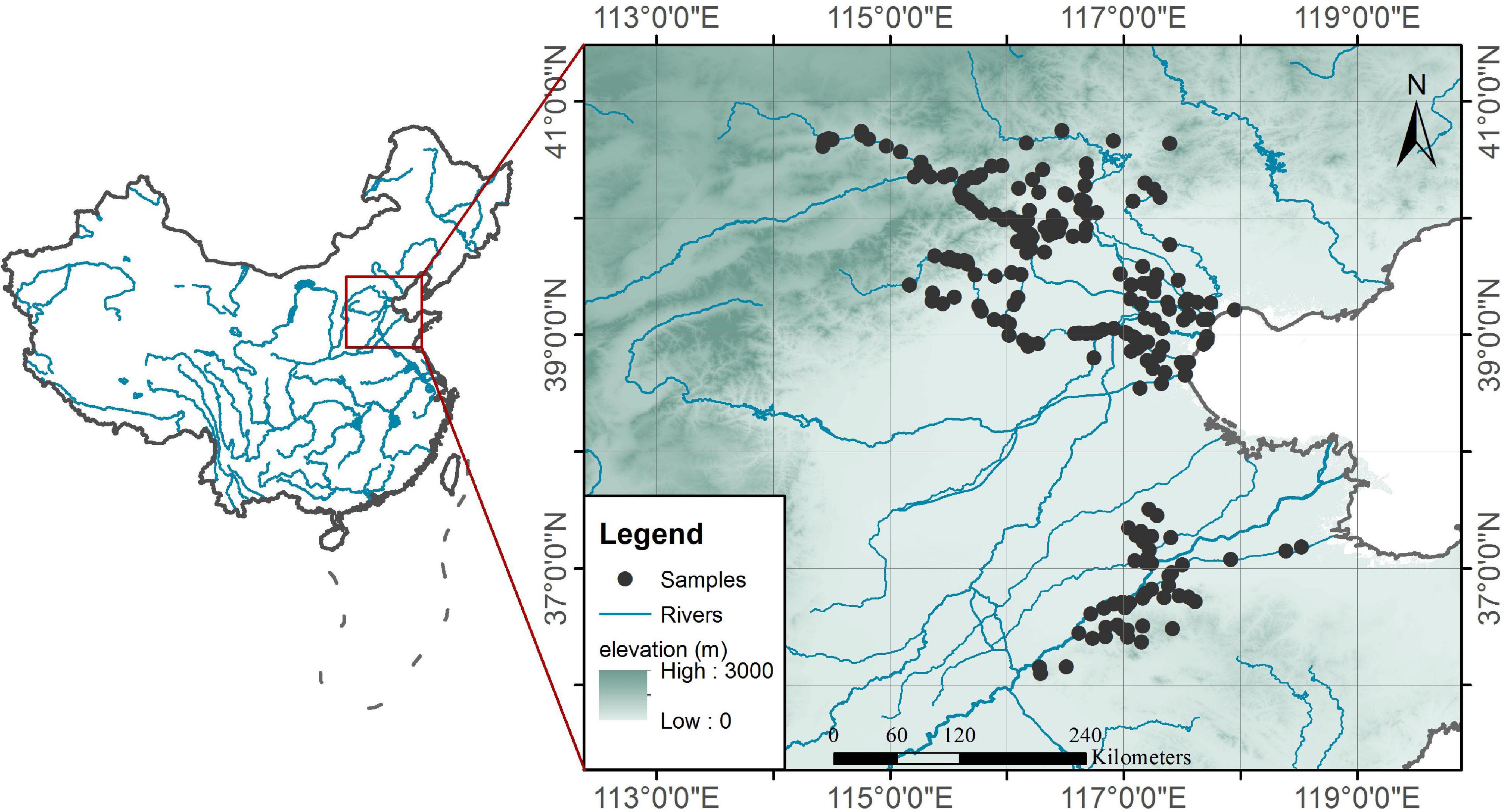
Figure 1. Spatial distribution of sampling sites.
The water temperatures at 0.2 m below the water surface were directly measured on site. The water samples were collected in 500-mL polyethylene plastic bottles and stored in an incubator filled with ice packs. After the sampling for each day was completed, the samples were sent back to the laboratory for analysis and determinations. The total phosphorus (TP) concentrations in the water samples were determined with the ammonium molybdate spectrophotometric method.
Water samples with volumes of 1,000 mL were taken from the middle depths of the reaches and were placed in polyethylene plastic bottles, shaken well, and 10–15 mL of Lugol’s iodine was added to fix the organisms. The water samples were left to settle for more than 48 h, the organisms that settled to the bottoms of the bottles were collected, and the volumes was adjusted to 50 mL. For the identification and counting of phytoplankton cells, 0.1 mL from a constant-volume sample was injected into a 0.1 mL chamber and counted with an optical microscope (CX21FS1, Olympus, Hatagaya, Tokyo, Japan) at 400 × resolution. The Protozoa and rotifers were identified and counted at 100–400 × resolution. The Protozoa were counted using a 0.1-mL chamber, and the rotifers and nauplii were counted using a 1-mL chamber. Each sample was counted twice, and the average was taken.
The identification and counting of cladocera and copepods were performed under a low-resolution microscope. Water sample with volumes of 10 L were collected and poured into a No. 25 plankton net for filtration, the concentrates were placed into 20-mL glass bottles, and 4% formalin was added to fix the organisms. The collected water samples were precipitated for 24 h, and the volumes were then adjusted to 30 mL. The identification and counting of copepods and cladocera were performed using a 5-mL chamber (Wang, 2011).
Piecewise regression is a regression estimation method that is applicable when two variables obey different linear relationships within different independent variable ranges (Toms and Lesperance, 2003; Toms and Villard, 2015). If the two variables (e.g., independent variable X and dependent variable Y) obey a simple linear relationship, the model is shown in Formula (1):
When X < X1, Y and X obey the simple linear relationship shown in Equation 1 and when X > X1, Y and X obey another linear relationship, its intercept and slope are significantly different from before, but Y is continuous at X1. Therefore, a dummy variable D is used to conform to the conditions of Formula (2):
The piecewise regression model between Y and X is shown in Formula (3):
According to Equation 3, when X is in different ranges, the expected values of Y are:
when
when
Segmented regression is a statistical method that is suitable for detecting breakpoints in “broken stick” models. Breakpoint detection was performed by using the Segmented package in R4.0.2. The working principle of Segmented package is described in the literature (Muggeo, 2008). The Segmented package can automatically provide the Akaike information criterion (AIC) values for evaluating the effect of segmented regression analysis, which is a standard used to measure the goodness of model fitting (Akaike, 1974). For the case of the same number of samples, the lower the AIC value is, the better the model fitting effect. In addition, to compare the reliability of the breakpoints that are determined by the segmented regression analysis, this paper uses the standard error (SE) and SE/Est. (the ratio of the standard error to the abscissa value of the breakpoint), which are automatically calculated by the Segmented package in R4.0.2 (R Development Core Team, Auckland, New Zealand). The lower the SE and SE/Est. values, the more reliable the breakpoint evaluation. If both the AIC value and the SE/Est. value are relatively low at the same time, it can indicate that the reliability of the threshold detection is relatively high.
An “L”-shaped scatter is a common type of bivariate scatter observed in the quantitative relationship analyses of aquatic ecosystems (Cade and Schroeder, 1999; Wang et al., 2007), as shown in Figure 2A. The distribution of this type of scatter has obvious change characteristics, that is, it is similar to the “broken stick” threshold type, but it cannot be determined by piecewise regression.
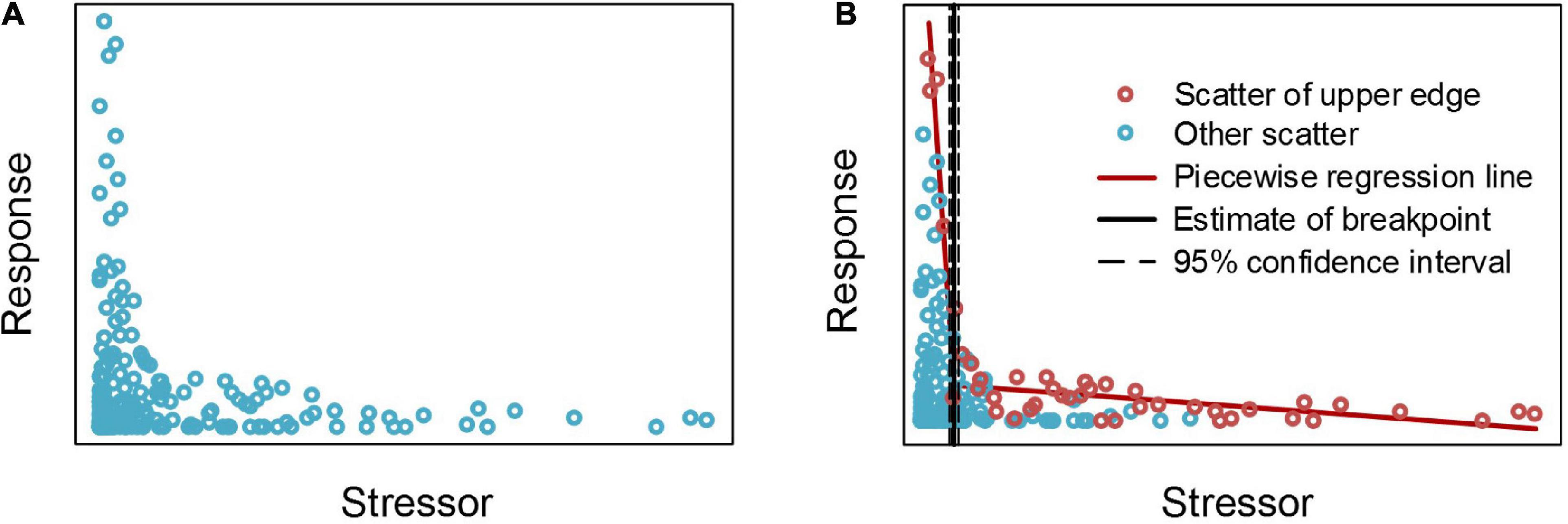
Figure 2. Segmented analysis results of “L” shaped simulated scattered points after selecting the edge scatter. Panel (A) shows simulation of “L” shaped scattered points, panel (B) shows the selection of the edge scatter points and the segmented analysis results of edge scatter points.
For this type of scatter, the boundary of the scatter is often determined, and then the abrupt point of the scatter distribution is estimated according to the breakpoint of the boundary (Brenden et al., 2008). The mainstream method that is used to determine the boundaries of scatter points is the quantile method, that is, using an appropriate cutting quantile to separate the edge scatter points that can describe the variations in the scatter distribution so that these scatter points can be fit for piecewise regression (Brenden et al., 2008; Qiu et al., 2021). However, for an “L” shaped scatter, as shown in Figure 2A, the right branch of the scatter plot is close to the horizontal axis, and the edge scatter cannot be obtained through the quantile cut as for the left.
In this paper, the maximum value is used as the upper boundary, that is, the horizontal axis is divided into several segments at equal intervals, and the scatter point with the largest ordinate value in each segment is taken as the edge scatter point (Figure 2B). These edge scatter points effectively reflect the change characteristics of the scatter point distribution and can indicate the changes in the maximum value of the ordinate when the abscissa moves from left to right or from right to left. The Segmented package is used to perform piecewise regression fitting on these selected edge scatter points to determine the threshold position of the “L” shaped scatter points.
Polynomial regression fitting analysis was used to investigate the change trends of the averages, standard deviations and coefficients of variation and to verify the validity of the threshold detection method. The average and standard deviation describe the concentrated characteristics of the scatter points. The smaller the standard deviation is, the more concentrated the scatter points are. In contrast, the larger the standard deviation is, the more scattered the scatter points are, which indicate a greater degree of scatter fluctuation. The coefficient of variation is the ratio of the standard deviation to the average, which offsets the influence of different average values and can more objectively reflect the degree of dispersion of the scatter points. The larger the coefficient of variation is, the greater the degree of fluctuation of the scatter points.
For the convenience of observation, we examined whether the amplitudes of the fluctuations in the cyanobacteria densities changed when the cladocera densities were close to the threshold and less than the threshold as the cladocera density changed from the maximum value to minimum value. The calculation process for the average, standard deviation, and coefficient of variation are as follows: starting from the first sample on the far right, calculate the average, standard deviation, and coefficient of variation for all samples on the right side of the abscissa as each integer bit, and record them at the corresponding abscissa as the integer bit. If there are no samples from n to n+k on the abscissa, no calculation is performed between them.
Before performing the threshold analysis, a preliminary observation was made of the distribution characteristics of each group of scatterplots. If the scatter distribution has a typical “L” shape, the analysis path of “finding edge scattered points-piecewise regression” can be used for threshold detection. If the scatter distribution do not have the characteristics of an “L” shape, threshold detections were not performed for these groups. To confirm whether cladocera is the key group for cyanobacterial control in zooplankton, the analysis was carried out using the screening idea of “whole to part.”
All sites are grouped according to the cladocera density and cyanobacterial density. The averages of the density and dominance among groups were compared by using one-way ANOVA followed by an LSD post hoc test. The assumptions of ANOVA were met because the homogeneity and normality were confirmed by Levene’s test and by the Kolmogorov–Smirnov test or Shapiro–Wilk test, respectively. The statistical analyses were performed using the Statistical Product and Service Solution (SPSS) 20 statistical package (International Business Machines Corporation, New York City, NY, United States).
According to the observations of the scattered points, (a), (b), (c), (d), (e), (f), and (g) in Figure 3 conform to this feature; therefore, threshold detection is performed on these seven groups of scatter points. However, the scatter plots in (h) and (i) do not have the characteristics of an “L” shape, so threshold detections were not performed for these two groups.
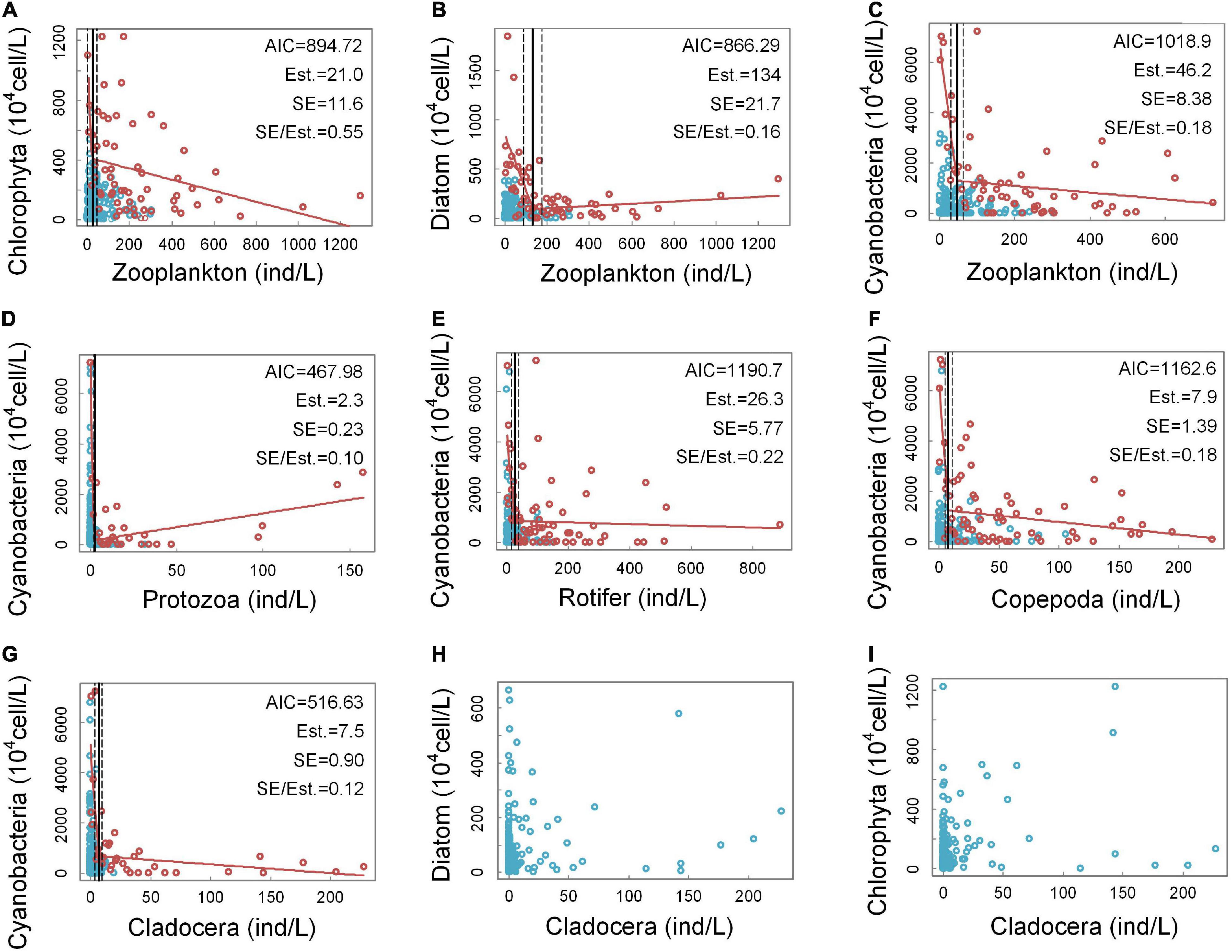
Figure 3. Quantitative relationships between the densities of the groups of zooplankton and phytoplankton. In panels (A–G), the horizontal axis intervals used in the selection of the edge scatter points are 5 ind/L, 5 ind/L, 5 ind/L, 1 ind/L, 2 ind/L, 2 ind/L, and 1 ind/L, respectively. In panel (D), a singular point with extremely high protozoan density is excluded. This sample point is located in Xinglin Reservoir, Jinan. At this site, the density of protozoa reached 888 ind/L, and the density of cyanobacteria was 723.8⋅104 cell/L. Panels (H–I) cannot select edge scatter points.
Figures 3A–C demonstrate the relationships between the densities of three dominant groups of phytoplankton (e.g., chlorophyta, diatoms, and cyanobacteria) and the overall density of zooplankton. From the AIC values, the piecewise regression fitting effect for (a) and (b) is slightly better than that for (c) and from the SE/Est. values, the breakpoint estimation effects of (b) and (c) are better. Judging from the fit between the fitting results of piecewise regressions and the scatter distribution characteristics, (b) and (c) have a high degree of fit, while (a) has a low degree of fit. In addition, the densities of the three phytoplankton groups indicate that cyanobacteria have the highest density and predominate among the phytoplankton. The relationship between zooplankton density and diatom density seems to have a relatively clear non-linear relationship, but the advantage that is occupied by diatoms in phytoplankton is limited, so cyanobacteria are mainly considered next.
Figures 3D–G show the quantitative relationships between the cyanobacteria densities and the four groups of zooplankton (e.g., protozoa, rotifer, copepoda, and cladocera). From the AIC values, the piecewise regression fitting effects of (d) and (g) are the best, while (d) and (g) have the relative lower SE/Est. values, which indicate that the breakpoint estimation effects are also the best. Judging from the fit between the fitting results of piecewise regression and the scatter distribution characteristics, the fits in (d), (e), (f), and (g) are all good, which indicate that the cyanobacteria densities have a clear non-linear relationship with the densities of the four zooplankton groups. Among them, (d) and (g) have the best fits. It can be seen from (d) that when the protozoan density is low, the values of the cyanobacteria density fluctuate greatly, and the scatter points with high cyanobacterial densities are all distributed in this range. The highest possible cyanobacterial density decreases rapidly as the protozoan density increases. However, as the density of protozoa continued to increase, the density of cyanobacteria began to increase significantly. From (e) and (f), it can be seen that the scatter points with higher cyanobacterial densities are located in the lower densities of rotifers and copepods. When the densities of rotifers and copepods were high, the maximum cyanobacterial densities decreased steadily but still maintained high levels. According to (g), the amplitudes of the cyanobacteria density fluctuations change when the cladocera density is approximately 7.5 ind/L. When the cladocera densities were lower than 7.5 ind/L, the amplitudes of the fluctuations in the cyanobacteria densities were very large, and the maximum value that the cyanobacteria density could reach dropped sharply from a very high level to a low level. When the cladocera density was greater than 7.5 ind/L, the cyanobacteria density decreased slowly with increasing cladocera density, and the amplitudes of the fluctuations in the cyanobacterial densities were small. The above results show that cladocera may be the most effective zooplankton group for controlling the abundance of cyanobacteria.
Figures 3H,I show the relationships between the cladocera density and the densities of diatoms and chlorophyta. According to (h) and (i), the scatter plots of diatom density-cladocera density and chlorophyta density-cladocera density did not have obvious “L”-shaped characteristics, so threshold detection was not performed.
The gray vertical solid line is the threshold position for cladocera controlling cyanobacteria detected in Figure 3G.
According to Figure 4, all three parameters have a common feature, namely, they all tend to increase as the cladocera density increases from large to small. When the cladocera densities reached different levels of low values, they all increased rapidly as the cladocera densities continued to decrease. Among them, the average growth rate began to increase significantly when the cladocera density was less than 50 ind/L. The standard deviation began to increase significantly when the cladocera density was less than 25 ind/L, and the standard deviation remained at a low level when the cladocera density was greater than 25 ind/L.
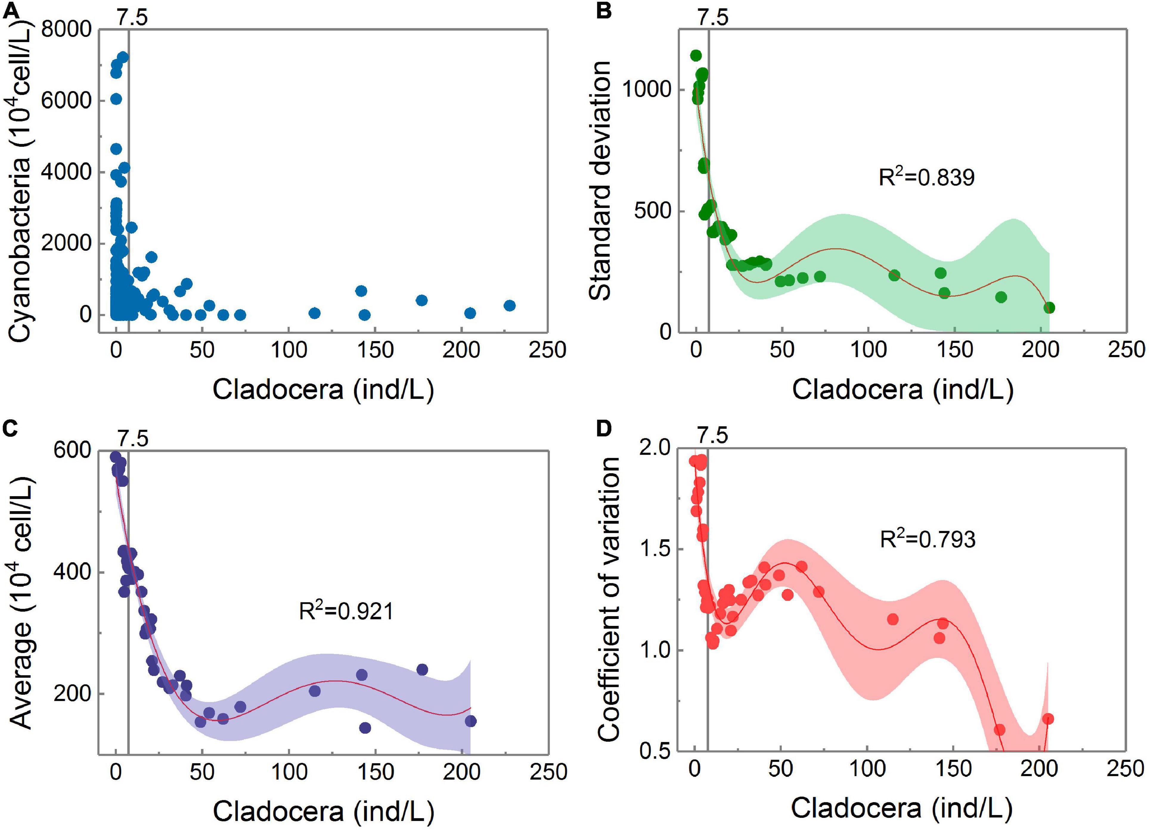
Figure 4. Panel (A) shows the scatter points of the Cladocera Density-Cyanobacteria Density. The trends of the dispersion degrees of the scatter points with changes in cladocera density. Panels (B–D) all adopt the polynomial fitting method, while panel (B) uses a 5th degree polynomial, panel (C) uses a 4th degree polynomial, and panel (D) uses a 6th degree polynomial. There is only one sample on the right side of the abscissa to 206 ind/L, and calculations of the average, standard deviation, and coefficient of variation are not performed.
Figure 4D shows that there are many locations where the coefficient of variation changes with changes in the cladocera density, but the location of the rapidly increasing change point when its value remains high is consistent with the location of the threshold detection shown in Figure 3G.
Figure 5 shows the body lengths of 37 cladocera that appeared in all samples. According to the body length order of all species, cladocera are classified as medium-large sized and micro-small sized (Figure 5). According to the threshold detection results shown in Figure 3G, all of the samples were divided into three groups (Figure 6). The average densities (Figure 6A) and average dominance (Figure 6B) of the medium-large and micro-small cladocera in each group were compared.
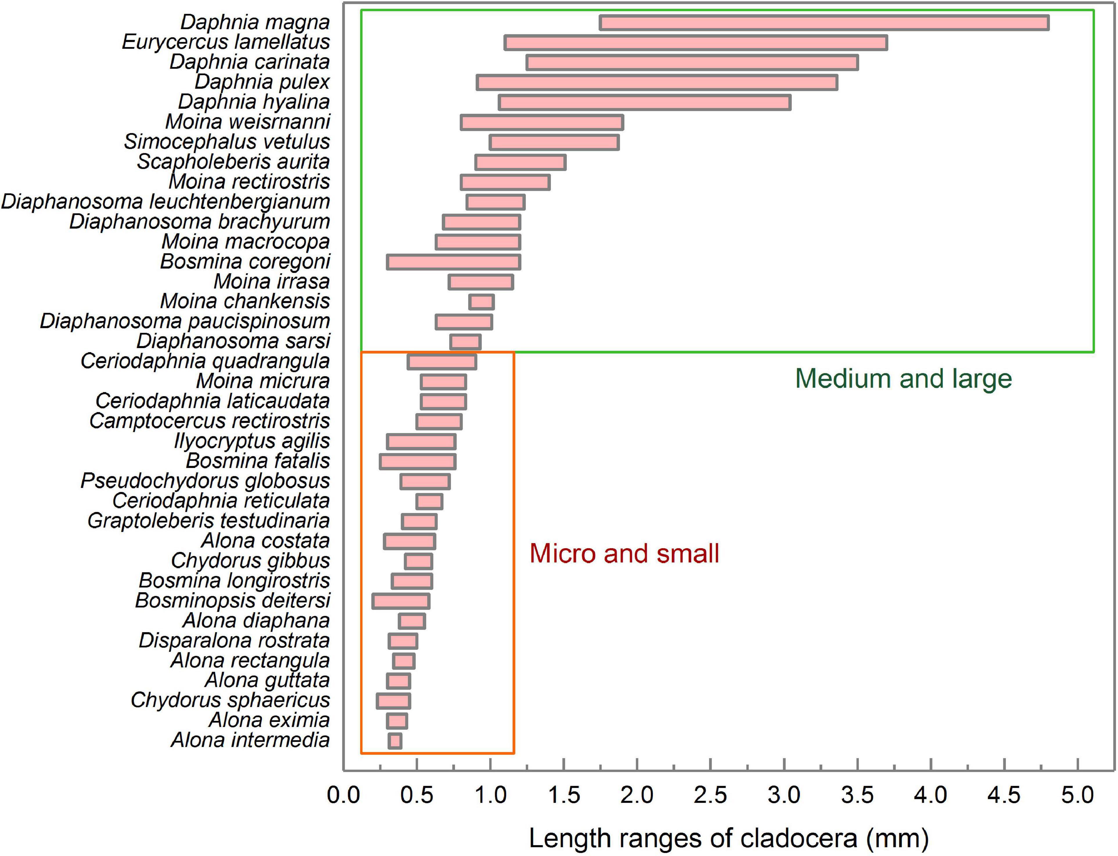
Figure 5. Length ranges and classification of various cladocera. The statistics for the body length range included both female and male individuals. The data for the cladocera body lengths come from the China Animal Scientific Database (http://www.zoology.csdb.cn/), which was jointly constructed by the Institute of Zoology, Chinese Academy of Sciences, Kunming Institute of Zoology, Chinese Academy of Sciences, Chengdu Institute of Biology, Chinese Academy of Sciences, Shanghai Entomological Museum, Chinese Academy of Sciences, and Institute of Hydrobiology, Chinese Academy of Sciences.
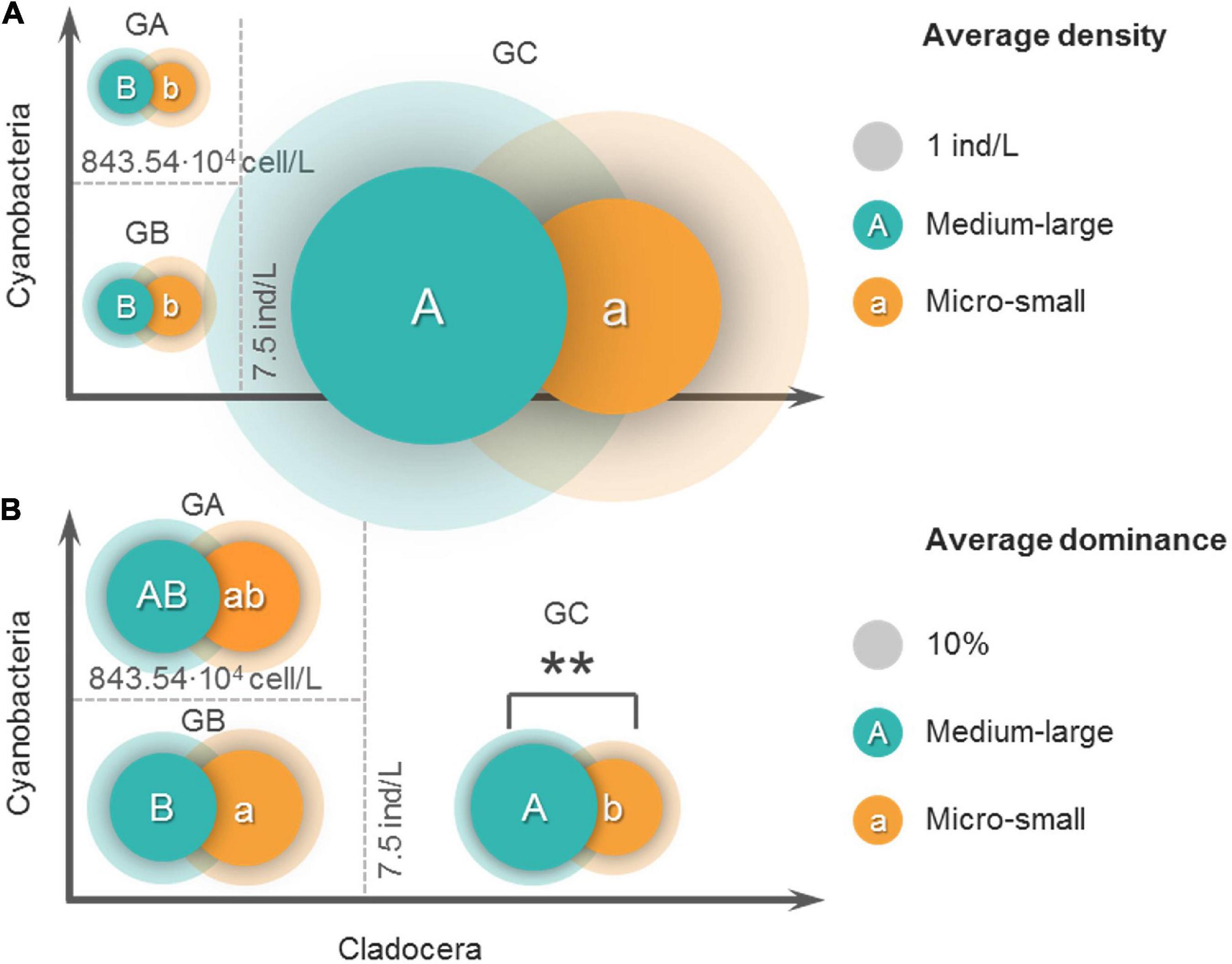
Figure 6. Comparisons of the average density (A) and average dominance (B) of the two sizes of cladocera in the three groups. Before grouping, the samples with zero cladocera density in the original samples were eliminated. All samples are divided into three groups based on the threshold value. GA: cladocera density < 7.5 ind/L (cladocera density corresponding to the breakpoint position of piecewise regression), and cyanobacteria density > 843.54 104 cell/L (cyanobacteria density corresponding to the breakpoint position of piecewise regression). GB: cladocera density < 7.5 ind/L and cyanobacteria density < 843.54 104 cell/L. GC: cladocera density > 7.5 ind/L. The capital letters A and B in the circles represent the results of the LSD post hoc test for the comparison among the groups of medium-large cladocera, and the lowercase letters a and b in the circles represent the LSD post hoc test results for the comparison among the groups of micro-small cladocera. The overlapping of two circles indicates that a comparison of the inner groups was carried out, ** indicates that the result of the comparison of the inner groups is extremely significant (P < 0.01), and those without ** indicate that the differences in the inner groups are not significant (P > 0.05). The opaque circles represent the average values, and the transparent rings represent the standard deviations. The areas of the circles and rings represent the averages and standard deviations, respectively.
According to the comparison of the average cladocera densities (Figure 6A), the results of the comparisons among groups showed that the average density of the GC group (30.3 ind/L, 18.3 ind/L) was highest for both medium-large and micro-small cladocera and was significantly (P < 0.01) greater than that of the GB group (1.24 ind/L, 1.46 ind/L) and GA group (1.16 ind/L, 1.04 ind/L). The difference between the GA and GB group was not significant (P > 0.05). The results of the comparisons of the inner groups showed that in the GA and GC groups, the average density of medium-large cladocera was greater than that of micro-small cladocera, but the difference was not significant (P > 0.05).
According to the comparison of the average dominance of cladocera (Figure 6B), the results of the comparisons among groups showed that for the medium-large cladocera, the average dominance in the GC group was largest (63.5%), which was significantly (P < 0.05) greater than that of the GB group (46.4%) and greater (51.5%) than that of the GA group but was not significant (P > 0.05). For micro-small cladocera, the average dominance of the GB group was largest (53.6%), which was significantly (P < 0.05) greater than that of the GC group (36.5%) and slightly greater than that of the GA (48.5%) group, but this difference was not significant (P < 0.05). The results of the comparisons of the inner groups showed that there were no significant differences (P > 0.05) in the average dominance of the medium-large and micro-small groups regardless of whether it was the GA or GB group. The average dominance of the medium-large cladocera in the GC group was significantly (P < 0.01) greater than that of micro-small cladocera.
In the threshold analysis, it is not enough to only consider differences in abundance and dominance of cladocera. It needs to be considered whether the lower cyanobacteria density in GC group is due to lower temperature or TP concentration, and whether the higher cyanobacteria density in GA group is due to higher temperature or TP concentration. The differences in water temperature and TP concentration among the three groups were examined below (Figure 7).
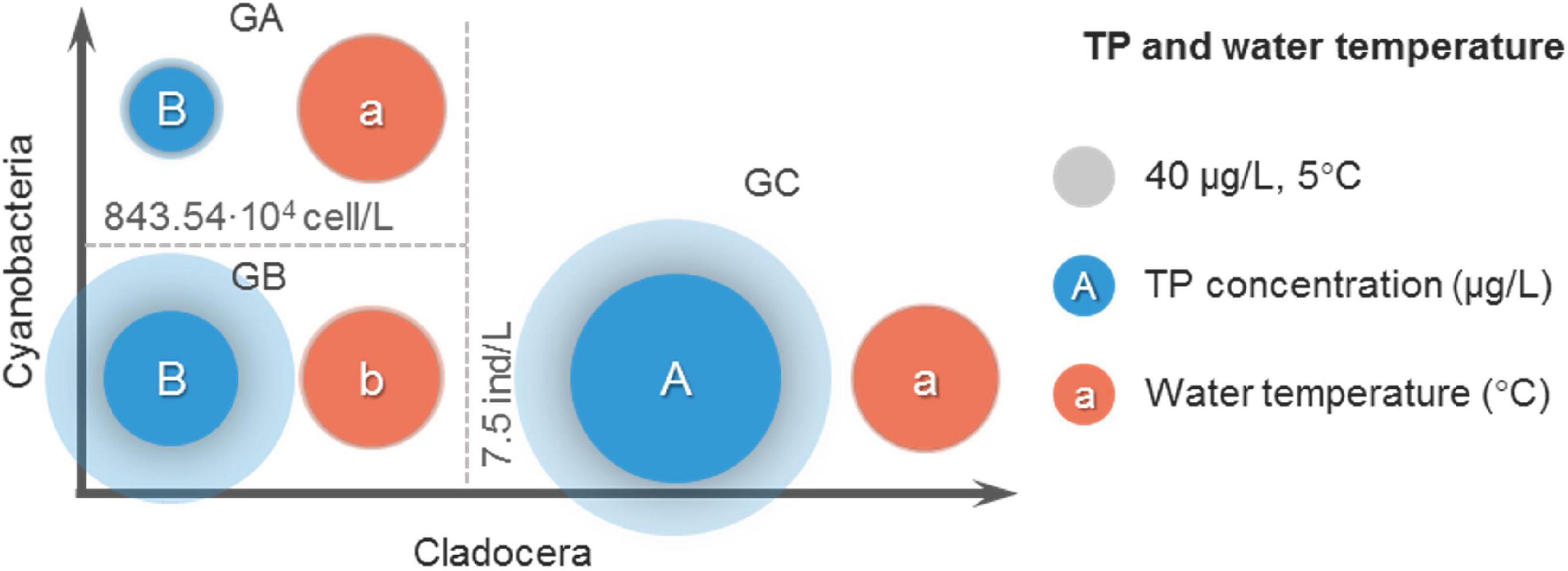
Figure 7. Average comparison of TP and water temperature among the three groups. No intragroup comparisons were made in this comparison.
According to the comparison of average TP concentrations (Figure 7), the average TP concentration of GC group was the largest (454 μg/L), and was significantly (P < 0.01) greater than that of GA group (72 μg/L) and GB group (186 μg/L). The average TP concentration in GA was less than that in GB group but not significant (P > 0.05). This suggests that the lower cyanobacteria density in the GC group was not caused by the lower TP concentration, instead, the TP concentration was greater in the GC group.
According to the comparison of average water temperature (Figure 7), the average water temperature of GB group was the lowest (23.4°C), and was significantly (P < 0.05) lower than that of GA group (26.5°C) and GC group (26.0°C). The average water temperature of the GA group was very close to that of the GC group (P > 0.05). This suggests that in the GC group, the lower cyanobacteria density was not due to temperature differences.
Detecting the abrupt changes in the quantitative relationships between pressure-response variables in the scatters of “L”-shaped distributions has always been a difficult problem in aquatic ecosystems. In this paper, we propose a threshold detection path of “finding edge scattered points-piecewise regression” to explore the non-linear relationship between zooplankton density and phytoplankton density. We confirm the accuracy of our adopted threshold detection method by observing the changes in the coefficient of variation. The results show that the position of the breakpoint that is obtained by the threshold detection analysis is consistent with the position of the change in the coefficient of variation, which demonstrates that the detection path of “finding edge scattered points-piecewise regression” is reliable in this study. In fact, in addition to the scatter of zooplankton-phytoplankton densities, scatter plots showing this “L”-shaped distribution are common in aquatic ecosystems (Cade and Schroeder, 1999; Wang et al., 2007). This type of scatter plot clearly shows a non-linear relationship between two variables. When the number of samples is sufficient, the analysis path proposed in this paper is an important threshold detection method that is worth considering.
This paper mainly studies the control effect of zooplankton on the phytoplankton abundance (especially cyanobacteria), and other important factors that affect cyanobacterial abundances need to be excluded during the analysis. Water temperatures, TP concentrations, and residence times are considered to be the main environmental factors that affect cyanobacterial abundances (Cha et al., 2017). In this paper, the sampling is limited to slow-flowing waters, so the effect of residence time on cyanobacteria abundance is not considered. We analyzed the interference effects of water temperatures and TP concentrations on the cyanobacterial control of cladocera. The results (Figure 7) showed that the average TP concentration in the GC group, with a lower cyanobacterial abundance, was significantly higher than that in the GA group with a high cyanobacterial abundance, while the average water temperature of the GC group was not significantly different from that of the GA group. This indicated that the lower cyanobacteria density in the GC group was not caused by water temperature or TP, which ruled out the interference of temperature or TP in this study. Some literatures indicate that bioavailability of nitrogen and phosphorus have different effects on the density of phytoplankton (Tarapchak and Moll, 1990). For example, the density of phytoplankton was highly related to the concentrations of nutrients of reactive nitrogen and phosphorus (Crossetti et al., 2013). The concentrations of various forms of nitrogen and phosphorus were not tested for this survey. The effect of reactive nitrogen and phosphorus on phytoplankton deserves consideration in subsequent studies.
The quantitative relationship between cyanobacterial abundance and cladocera density may not only be the result of predation by cladocera, but the adaptation of cladocera to cyanobacteria may also have an important impact on this relationship. Some studies suggest that high abundance of cyanobacteria and cyanobacterial toxins will threaten the survival of cladocera (Jiang et al., 2013; Amorim and Moura, 2021), and the density of cladocera may be reduced. At the same time, under the pressure of the harsh external environment, the reproduction and growth strategies of cladocera have changed significantly, and the cladocera will tend to be dominated by small individuals (Li et al., 2017). These could be another explanation for the inverse correlation of cyanobacterial abundance in cladocera densities, as well as differences in cladocera size among groups (i.e., GA, GB, GC groups).
Zooplankton is recognized as a key biological group for algae control (Bernardi et al., 1987; Amorim and Moura, 2020), and it is very important for the ecological restoration of eutrophic lakes to identify the most effective groups for cyanobacteria control in zooplankton. In addition, since most of the previous studies focused on the abundance or biomass of zooplankton or phytoplankton as a whole, such binary quantitative relationship analysis is often difficult to identify non-linear characteristics in complex systems. Based on the threshold detection and the screening of groups, the analysis results in this paper support that in wild ecosystems, cladocera may be the group with the strongest ability to control the abundance of cyanobacteria in zooplankton.
Although the reliability of threshold detection in protozoa-cyanobacteria is good, the cyanobacteria density eventually increases with the increase of protozoa density, which indicated that the potential control effect of protozoa on cyanobacteria was unstable. Both rotifer and copepod seem to have some control effect on cyanobacteria density, but the larger AIC and SE/Est. values suggest that the potential control effect is not very significant. Cladocera seem to have the best control ability on cyanobacteria abundance. When the cladocera density was greater than 7.5 ind/L, the cyanobacteria density was maintained at a very low level, and the maximum cyanobacteria density decreased slowly with the increase of cladocera density. When the cladocera density changes from large to small, and the density is close to or less than 7.5 ind/L, the fluctuation amplitude of the cyanobacteria density begins to increase rapidly. This shows that the control effect of cladocera on cyanobacteria is non-linear as the cladocera abundance changes. In fact, similar non-linear changes may exist in many forms in aquatic ecosystems. Through the quantitative study of these non-linear changes, it may be easier to reveal the mechanism of complex change in the whole system.
Through the comparative analysis of grouped samples based on thresholds, the results of this study show that in wild ecosystems, the cladocera-cyanobacteria predation relationship generally follows the “size-efficiency” hypothesis. However, the role of cladocera body size in cyanobacteria control is not very prominent. In the GC group (the samples in which the cyanobacteria abundances were effectively controlled), the average dominance of medium-large cladocera was significantly greater than that of micro-small cladocera (P < 0.01). The average dominance of medium-large cladocera in the GC group was greater than that in the GA group (the samples in which cyanobacteria abundance was uncontrolled), but the difference was not significant (P > 0.05). In addition, the average density of medium-large cladocera in the GC group was higher than that of micro-small cladocera, and the difference was not significant (P > 0.05). This result indicates that when cladocera control the abundance of cyanobacteria, the role of medium-large cladocera is indeed greater than that of micro-small cladocera, but this gap is not overwhelming, and micro-small cladocera also play an important role. This result suggests that the benefits of ecological governance strategies by pursuing the proportion of large cladocera among cladocera may be limited.
The overall abundances of cladocera in wild ecosystems may have a greater impact than individual body sizes on the control efficiency of cyanobacteria abundances. In fact, the average densities of both medium-large cladocera and micro-small cladocera were much larger in the GC group than in the GA group (Figure 6A). This indicates that the higher density of cladocera may be the overwhelming reason for the effective control of cyanobacteria abundances in the GC group. This means that in wild ecosystems, cladocera can effectively control cyanobacteria abundances and depend on sufficient densities, regardless of the proportions of large cladocera. That is, the strategy that cladocera may adopt when controlling cyanobacteria is “win by quantity” rather than “win by size.”
The above analysis suggests that increasing the abundances of cladocera should be considered a priority when restoring zooplankton communities to reduce the risk of cyanobacteria blooms in temperate freshwater ecosystems. Increasing the density of cladocera above 7.5 ind/L can be an important goal of water environment management. In slow-flowing waters, the greater the abundance of cyanobacteria is, the higher the risk of cyanobacteria blooms. According to the results of analyzing 242 sampling points in North China (Figure 3G), when the cladocera density is greater than 7.5 ind/L, cladocera can effectively control the cyanobacteria abundance to a low level, which significantly reduces the risk of cyanobacteria blooms. When the cladocera densities fell below this threshold, the likelihood of cyanobacteria blooms rose rapidly. Therefore, cladocera densities that are close to or below the threshold can be used as an important signal for early warnings of cyanobacterial blooms. It should be noted that lower cladocera densities do not necessarily mean that cyanobacteria will grow rapidly or that blooms will occur. Even with very low cladocera densities, the cyanobacteria densities may be very low (Figure 3G). This means that although the cladocera densities may be able to predict the changing trends of the fluctuations in cyanobacteria abundance, they cannot predict the specific cyanobacteria abundance values in wild ecosystems. In addition, the predation of cladocera on cyanobacteria and the species/morphotypes response strategies of cladocera to cyanobacterial differ in different climate regions (Jeppesen et al., 2020; Amorim et al., 2020). Therefore, studies on the quantitative relationship between cladocera and cyanobacteria in different climatic regions may yield significantly different conclusions.
The unique non-linear relationship between the cladocera density and cyanobacteria density can be well explained by chaos theory. Chaos theory holds that when the external pressure crosses a certain threshold, the system state bifurcates, and the system enters a chaotic state from a stable state (May, 1976; Scheffer, 2009). After entering a chaotic state, even small differences in the initial conditions will eventually cause very large differences in the system state over time. For the case analyzed in this paper, the sites had similar water temperatures in both the GA and GC groups and even higher nutrient levels in the GC group, and in fact, these sites had the potential for cyanobacterial blooms. However, in the GC group, due to the high cladocera densities, these cladocera maintained a strong predation ability on cyanobacteria, the potential for cyanobacteria to grow rapidly was suppressed, and the amplitudes of the fluctuations in cyanobacteria densities remained within a very small range. When the cladocera density was below the threshold value, the predation effect of cladocera on cyanobacteria was not sufficient to offset the effects of other environmental conditions on the cyanobacteria density. As the cladocera density decreased, the effects of the differences in initial environmental conditions (such as TP, and water temperature) on the cyanobacteria density increased almost exponentially. The amplitudes of the fluctuations in cyanobacteria density increase sharply, which is a phenomenon that indicates that the cladocera density cannot be used to constrain and predict cyanobacteria abundances. The cyanobacteria control threshold of cladocera may be the critical point at which the cladocera-cyanobacteria predation relationship changes from a stable state to a chaotic state.
According to the above description, we cannot predict the specific values of cyanobacteria densities based on cladocera when the cladocera densities are very low. However, even in the “chaotic” state, we can still see that the maximum cyanobacterial density can reach a clear boundary, that is, the amplitudes of the fluctuations in the cyanobacteria densities can be predicted. This means that although precise predation dynamics cannot be predicted, the ranges of these predation behaviors can be described and can be predicted to remain constant as long as external conditions do not change (Scheffer, 2009). In fact, there are many non-linear relationships that are similar to the cladocera-cyanobacteria relationship, and more non-linear studies should be conducted in the future to reveal the complex mechanisms in natural aquatic ecosystems and improve the human ability to understand and respond to complex changes.
Ecological thresholds need to be verified by a large number of data and cases in order to achieve successful management applications. Although this paper investigates a large number of sample sites, this conclusion is limited to specific regions and climatic conditions. In the future, the quantitative non-linear relationship between cladocera and cyanobacteria should be verified under more climate types to obtain more general rules.
The purpose of this paper is to obtain a quantitative relationship between cladocera and cyanobacteria in wild ecosystems. According to the verification results of the coefficient of variation, the threshold detection path of “finding edge scattered points-piecewise regression” proposed by us is an effective method for detecting the tipping points in “L”-shaped scatters. The results of the screening analysis of groups showed that cladocera comprised the group with the best ability to control cyanobacterial abundances among zooplankton. The threshold detection results showed that the changes in cyanobacterial density with changes in cladocera density had obvious non-linear characteristics. There is a specific cladocera density (7.5 ind/L); when the cladocera density is less than this critical point, the amplitudes of the fluctuation in cyanobacteria densities will increase sharply. The analysis of TP and water temperature showed that these two important environmental conditions did not have significant disturbing effects in the analysis in this paper. The results of the analysis of the effect of body size shows that the body sizes of cladocera do play a role in controlling the cyanobacteria density, but the most critical factor for the success of cyanobacterial control is the greater density, rather than the dominance of large cladocera. Our study provides some evidence for understanding the complex changes in aquatic ecosystems, especially the occurrences and control mechanisms of cyanobacterial blooms. The threshold for cladocera being able to control cyanobacteria proposed by us may have important application value in water environment management. This threshold also provides a quantitative standard for early warnings of cyanobacteria blooms in temperate, shallow, and slow-flowing rivers.
The raw data supporting the conclusions of this article will be made available by the authors, without undue reservation.
DL: conceptualization, data curation, formal analysis, investigation, methodology, resources, software, validation, and writing—original draft. PH: conceptualization, investigation, funding acquisition, methodology, supervision, validation, and writing—review and editing. CL and JX: writing—review and editing and investigation. LH, XG, DW, and JW: writing—review and editing. All authors contributed to the article and approved the submitted version.
This research was funded by Biodiversity Survey and Assessment Project of the Ministry of Ecology and Environment, China (2019HJ2096001006).
The authors declare that the research was conducted in the absence of any commercial or financial relationships that could be construed as a potential conflict of interest.
All claims expressed in this article are solely those of the authors and do not necessarily represent those of their affiliated organizations, or those of the publisher, the editors and the reviewers. Any product that may be evaluated in this article, or claim that may be made by its manufacturer, is not guaranteed or endorsed by the publisher.
We would like to thank Junxia Wang, Yajuan Zhang, Chunchen Li, Mingyao Li, Shiwei Shan, and others for their assistance in the field survey.
Akaike, H. T. (1974). A new look at the statistical model identification. IEEE Trans. Automat. Contr. 19, 716–723. doi: 10.1007/978-1-4612-1694-0_16
Amorim, C. A., and Moura, A. N. (2020). Effects of the manipulation of submerged macrophytes, large zooplankton, and nutrients on a cyanobacterial bloom: a mesocosm study in a tropical shallow reservoir. Environ. Pollut. 265:114997. doi: 10.1016/j.envpol.2020.114997
Amorim, C. A., and Moura, A. N. (2021). Ecological impacts of freshwater algal blooms on water quality, plankton biodiversity, structure, and ecosystem functioning. Sci. Total Environ. 758:143605. doi: 10.1016/j.scitotenv.2020.143605
Amorim, C. A., Dantas, ÊW., and Moura, A. N. (2020). Modeling cyanobacterial blooms in tropical reservoirs: the role of physicochemical variables and trophic interactions. Sci. Total Environ. 744:140659. doi: 10.1016/j.scitotenv.2020.140659
Bernardi, R. D., Giussani, G., and Manca, M. (1987). Cladocera: predators and prey. Hydrobiologia 145, 225–243. doi: 10.1007/BF02530284
Brenden, T. O., Wang, L., and Su, Z. (2008). Quantitative identification of disturbance thresholds in support of aquatic resource management. Environ. Manag. 42, 821–832. doi: 10.1007/s00267-008-9150-2
Cade, B. S., and Schroeder, T. R. L. (1999). Estimating effects of limiting factors with regression quantiles. Ecology 80, 311–323.
Cha, Y. K., Cho, K. H., Lee, H., Kang, T., and Kim, J. H. (2017). The relative importance of water temperature and residence time in predicting cyanobacteria abundance in regulated rivers. Water Res. 124, 11–19. doi: 10.1016/j.watres.2017.07.040
Crossetti, L. O., Becker, V., Cardoso, L., de, S., Rodrigues, L. R., da Costa, L. S., et al. (2013). Is phytoplankton functional classification a suitable tool to investigate spatial heterogeneity in a subtropical shallow lake? Limnologica 43, 157–163. doi: 10.1016/j.limno.2012.08.010
Czyewska, W., Piontek, M., and Luszczyńska, K. (2020). The occurrence of potential harmful cyanobacteria and cyanotoxins in the Obrzyca river (Poland), a source of drinking water. Toxins 12:284. doi: 10.3390/toxins12050284
Gliwicz, M. Z. (1990). Food thresholds and body size in cladocerans. Nature 343, 638–640. doi: 10.1038/343638a0
Hall, D. J., Threlkeld, S. T., Burns, C. W., and Crowley, P. H. (1976). The size-efficiency hypothesis and the size structure of zooplankton communities. Annu. Rev. Ecol. Syst. 7, 177–208. doi: 10.1146/annurev.es.07.110176.001141
Hayes, N. M., and Vanni, M. J. (2018). Microcystin concentrations can be predicted with phytoplankton biomass and watershed morphology. Inland Waters 8, 273–283. doi: 10.1080/20442041.2018.1446408
Huertas, M. J., and Mallén-Ponce, M. J. (2021). Dark side of cyanobacteria: searching for strategies to blooms control. Microb. Biotechnol. 15, 1321–1323. doi: 10.1111/1751-7915.13982
Huisman, J., Codd, G. A., Paerl, H. W., Ibelings, B. W., Verspagen, J. M. H., and Visser, P. M. (2018). Cyanobacterial blooms. Nat. Rev. Microbiol. 16, 471–483. doi: 10.1038/s41579-018-0040-1
Jeppesen, E., Canfield, D. E., Bachmann, R. W., Søndergaard, M., Havens, K. E., Johansson, L. S., et al. (2020). Toward predicting climate change effects on lakes: a comparison of 1656 shallow lakes from Florida and Denmark reveals substantial differences in nutrient dynamics, metabolism, trophic structure, and top-down control. Inland Waters 10, 197–211. doi: 10.1080/20442041.2020.1711681
Jiang, X., Liang, H., Yang, W., Zhang, J., Zhao, Y., Chen, L., et al. (2013). Fitness benefits and costs of induced defenses in Daphnia carinata (Cladocera: Daphnidae) exposed to cyanobacteria. Hydrobiologia 702, 105–113. doi: 10.1007/s10750-012-1312-9
Jing, L., Parkefelt, L., Persson, K. M., and Pekar, H. (2017). Improving cyanobacteria and cyanotoxin monitoring in surface waters for drinking water supply. J. Water Secur. 3, 1–8. doi: 10.15544/jws.2017.005
Li, Y., Xie, P., Zhang, J., Tao, M., and Deng, X. (2017). Effects of filter-feeding planktivorous fish and cyanobacteria on structuring the zooplankton community in the eastern plain lakes of China. Ecol. Eng. 99, 238–245. doi: 10.1016/j.ecoleng.2016.11.040
Liang, Z., Soranno, P. A., and Wagner, T. (2020). The role of phosphorus and nitrogen on chlorophyll a: evidence from hundreds of lakes. Water Res. 185:116236. doi: 10.1016/j.watres.2020.116236
May, R. M. (1976). Simple mathematical models with very complicated dynamics. Nature 261, 459–467. doi: 10.1038/261459a0
Michalak, A. M., Anderson, E. J., Beletsky, D., Boland, S., Bosch, N. S., Bridgeman, T. B., et al. (2013). Record-setting algal bloom in Lake Erie caused by agricultural and meteorological trends consistent with expected future conditions. Proc. Natl. Acad. Sci. U S.A. 110, 6448–6452. doi: 10.1073/pnas.1216006110
Muggeo, V. (2008). Segmented: an R package to fit regression models with broken-line relationships. R News 8, 20–25.
Paerl, H. W., Xu, H., Mccarthy, M. J., Zhu, G., Qin, B., Li, Y., et al. (2011). Controlling harmful cyanobacterial blooms in a hyper-eutrophic lake (Lake Taihu, China): the need for a dual nutrient (N & P) management strategy. Water Res. 45, 1973–1983. doi: 10.1016/j.watres.2010.09.018
Peretyatko, A., Teissier, S., Backer, S. D., and Triest, L. (2012). Biomanipulation of hypereutrophic ponds: when it works and why it fails. Environ. Monit. Assess. 184:1517. doi: 10.1007/s10661-011-2057-z
Pick, F. R. (2016). Blooming algae: a Canadian perspective on the rise of toxic cyanobacteria. Can. J. Fish. Aquat. Sci. 73, 1–10. doi: 10.1139/cjfas-2015-0470
Postel, S., and Carpenter, S. R. (1997). Freshwater Ecosystem Services. Washington, DC: Island Press.
Qiu, Q., Liang, Z., Xu, Y., Matsuzaki, S. S., Komatsu, K., and Wagner, T. (2021). A statistical framework to track temporal dependence of chlorophyll–nutrient relationships with implications for lake eutrophication management. J. Hydrol. 603:127134. doi: 10.1016/j.jhydrol.2021.127134
Scheffer, M. (2009). Critical Transitions in Nature and Society. Princeton, NJ: Princeton University Press. doi: 10.1515/9781400833276
Shan, B. Q., Jian, Y. X., Tang, W. Z., and Zhang, H. (2012). Temporal and spatial variation of nitrogen and phosphorus and eutrophication assessment in downstream river network areas of north Canal River Watershed. Environ. Sci. 33, 352–358. doi: 10.13227/j.hjkx.2012.02.017
Shapiro, J., Lamarra, V., and Lynch, M. (1975). “Biomanipulation: An ecosystem approach to lake restoration. Water quality management through biological control,” in Proceedings of a Symposium on Water Quality Management Through Biological Control, eds P. L. Brezonik and J. L. Fox (Gainesville, FL: University of Florida), 85–96.
Shen, P. P., Shi, Q., Hua, Z. C., Kong, F. X., and Chen, D. C. (2003). Analysis of microcystins in cyanobacteria blooms and surface water samples from Meiliang Bay, Taihu Lake, China. Environ. Int. 29, 641–647. doi: 10.1016/S0160-4120(03)00047-3
Tarapchak, S. J., and Moll, R. A. (1990). Phosphorus sources for phytoplankton and bacteria in Lake Michigan. J. Plankton Res. 12, 743–758. doi: 10.1093/plankt/12.4.743
Toms, J. D., and Lesperance, M. L. (2003). Piecewise regression: a tool for identifying ecological thresholds. Ecology 84, 2034–2041. doi: 10.1890/02-0472
Toms, J. D., and Villard, M. A. (2015). Treshold detection: matching statistical methodology to ecological questions and conservation planning objectives. Avian Conserv. Ecol. 10, 51–57. doi: 10.5751/ACE-00715-10010
Wang, L., Robertson, D. M., and Garrison, P. J. (2007). Linkages between nutrients and assemblages of macroinvertebrates and fish in wadeable streams: implication to nutrient criteria development. Environ. Manag. 39, 194–212. doi: 10.1007/s00267-006-0135-8
Wang, Q. (2011). Using Submerged Macrophytes As Water Quality Indicators In Typical Regions of Haihe Rivers Basin. Beijing: Beijing Normal University.
Zhang, H., Lin, C., Lei, P., Shan, B. Q., and Zhao, Y. (2015). Evaluation of river eutrophication of the Haihe River Basin. Acta Sci. Circumst. 35, 2336–2344. doi: 10.13671/j.hjkxxb.2015.0025
Keywords: cladocera, cyanobacteria blooms, eutrophication control, ecological threshold, wild ecosystem, aquatic ecosystems
Citation: Li D, He P, Liu C, Xu J, Hou L, Gao X, Wang D and Wang J (2022) Quantitative relationship between cladocera and cyanobacteria: A study based on field survey. Front. Ecol. Evol. 10:915787. doi: 10.3389/fevo.2022.915787
Received: 08 April 2022; Accepted: 27 June 2022;
Published: 14 July 2022.
Edited by:
Xiaodong Qu, China Institute of Water Resources and Hydropower Research, ChinaReviewed by:
Yuying Li, Nanyang Normal University, ChinaCopyright © 2022 Li, He, Liu, Xu, Hou, Gao, Wang and Wang. This is an open-access article distributed under the terms of the Creative Commons Attribution License (CC BY). The use, distribution or reproduction in other forums is permitted, provided the original author(s) and the copyright owner(s) are credited and that the original publication in this journal is cited, in accordance with accepted academic practice. No use, distribution or reproduction is permitted which does not comply with these terms.
*Correspondence: Ping He, aGVwaW5nQGNyYWVzLm9yZy5jbg==
†These authors have contributed equally to this work and share first authorship
Disclaimer: All claims expressed in this article are solely those of the authors and do not necessarily represent those of their affiliated organizations, or those of the publisher, the editors and the reviewers. Any product that may be evaluated in this article or claim that may be made by its manufacturer is not guaranteed or endorsed by the publisher.
Research integrity at Frontiers
Learn more about the work of our research integrity team to safeguard the quality of each article we publish.