 Md. Omar Sarif
 Manjula Ranagalage
 Rajan Dev Gupta
 Yuji Murayama
94% of researchers rate our articles as excellent or good
Learn more about the work of our research integrity team to safeguard the quality of each article we publish.
Find out more
ORIGINAL RESEARCH article
Front. Ecol. Evol., 18 May 2022
Sec. Environmental Informatics and Remote Sensing
Volume 10 - 2022 | https://doi.org/10.3389/fevo.2022.901156
This article is part of the Research TopicEarth Observation Systems for the Urban Environment and Climate ChangeView all 5 articles
Many world cities have been going through thermal state intensification induced by the uncertain growth of impervious land. To address this challenge, one of the megacities of South Asia, Bengaluru (India), facing intense urbanization transformation, has been taken up for detailed investigations. Three decadal (1989–2019) patterns and magnitude of natural coverage and its influence on the thermal state are studied in this research for assisting urban planners in adopting mitigation measures to achieve sustainable development in the megacity. The main aim of this research is to monitor the surface urban cool island (SUCI) in Bengaluru city, one of the booming megacities in India, using Landsat data from 1989 to 2019. This study further focused on the analysis of land surface temperature (LST), bare surface (BS), impervious surface (IS), and vegetation surface (VS). The SUCI intensity (SUCII) is examined through the LST difference based on the classified categories of land use/land cover (LU/LC) using urban-rural grid zones. In addition, we have proposed a modified approach in the form of ISBS fraction ratio (ISBS–FR) to cater to the state of urbanization. Furthermore, the relationship between LST and ISBS–FR and the magnitude of the ISBS–FR is also analyzed. The rural zone is assumed based on <10% of the recorded fraction of IS (FIS) along the zones in the urban-rural gradient (URG). It is observed that SUCII hiked by 1.92°C in 1989, 4.61°C in 2004, and 2.66°C in 2019 between demarcated urban and rural zones along URG. Furthermore, the results indicate a high expansion of impervious space in the city from 1989 to 2019. The alteration in the city landscape mostly occurs due to impervious development, causing the intensification of SUCI. The mean LST (MLST) has a negative relationship with the fraction of VS (FVS) and a positive relationship with the fraction of BS (FBS). In addition, the ISBS–FR shows intense enlargement. The findings of the present study will add to the existing knowledge base and will serve as a road map for urban and landscape planning for environmental enrichment and sustainability of the megacity of Bengaluru.
Globally, it is estimated that 54.5% of the total population in the world lived in urban areas in 2016 and that 60% of the population will live in urban areas in 2030 if the same trend continues (United Nations, Department of Economic and Social Affairs, Policy Division, 2016). As per the IPCC (2019), the global land surface temperature (LST) and global (ocean and land) mean surface air temperature amplified by 1.53 and 0.87°C, respectively, between the preindustrial period (1850–1900) and the recent postindustrial period (2006–2015). In the last five decades, the coverage of urban settlements has rapidly increased, and a colossal transformation has taken place in land use/land cover (LU/LC) through natural land into the concrete structure, which led to changes in the local environment, resulting in the formation of a large elevated surface temperature as compared to its surrounding rural area (Kikon et al., 2016; Wang et al., 2018; Vinayak et al., 2022). This variation pattern of temperature, which intensifies warmer scenarios in the city center than in surrounding rural places, is called surface urban heat island (SUHI) (Shahfahad et al., 2021, 2022b). In reverse, when the surrounding rural places observe warmer scenarios than the city center, it is called surface urban cool island (SUCI) (Yang et al., 2017). SUCI formation is characterized by lower temperatures over a metropolitan area or a core urban center than in suburban areas or rural areas due to the semiarid effects of urbanization (Frey et al., 2005; Govind and Ramesh, 2019). The variation in temperature over the urban–rural difference occurs due to the conversion of the natural land surface, such as shrinkage of water bodies, deforestation, and depletion of farmland, into the concrete jungle and purely impervious surface (IS) due to urbanization (Chakraraborty et al., 2015; Ranagalage et al., 2017, 2018a; Dissanayake et al., 2019a; Naikoo et al., 2020).
The knowledge of LU/LC pattern has facilitated in carrying out urban morphology, ecology, sustainability, and geography by analyzing the pattern of land use, urban intensity, SUHI, SUCI, and urban diversity (Siddiqui et al., 2021; Rahman et al., 2022; Shahfahad et al., 2022a). The dynamics of LU/LC encourage a more extensive course of urban planning for health authorities, policymakers, urban investors, urban planners, and other scientific communities due to its harmful impacts on the health of the urban people as well as the alteration in precipitation, temperature, store carbon, air quality, and energy balance (Wang et al., 2017; Ranagalage et al., 2018c; Rousta et al., 2018).
Due to manmade reasons, the presence of inheriting distinct characteristics of the physical surface in the city landscape leads to the constitution of a wide variety of patterns in the form of absorption of electromagnetic radiation, longwave albedo radiation, evaporation, the release of heat, and prevailing wind blockage (Bokaie et al., 2016). The physical surfaces of urban landscape are widely different because these are the creation of stones, asphalt, gravel, pebbles, concrete, and flooring, which largely accelerate the sensitivity and lower evapotranspiration, which greatly spurs the local climate in the city landscape (Mirzaei, 2015; Rousta et al., 2018). Consequently, significant variation of LST has been perceived.
Previously, most of the literature related to stocktickerUCI studies have been focused on various city types, especially in tropical and semiarid cities, such as Abu Dhabi and Dubai, Chang–Zhu–Tan, Erbil, and Bengaluru (Frey et al., 2005; Li et al., 2011; Rasul et al., 2016, 2017; Govind and Ramesh, 2019). The SUCI is one of the essential phenomena which is created due to changing scenarios of the local environment in the densely urban set–up in semi–arid regions. However, unlike SUHI, SUCI has not been explored in other parts of the world in an intensive and extensive style (Li et al., 2011; Rasul et al., 2016). The SUCI played a vital role in the local atmosphere whose effects can be seen in the aspects of nature (such as macroorganisms to microorganisms) and animal life, including humans. SUCI is extending over the suburban/rural space at higher temperature magnitudes as compared to its core urban space due to the presence of recreational and biological parks where a large number of trees, water bodies in the form of small to big size ponds/lakes, and green lawns are available (Govind and Ramesh, 2019). SUCI has significantly pulled the attention of urban planners, urban investors, health authorities, and policymakers to its hostile effects on the life of humans and the environment.
Therefore, the strategy for the mitigation of SUCI must be introduced by studying the dynamics of the city’s landscape through spatial analysis to cope with its adverse effects. In the recent past, the use of environment-friendly raw materials and proper design of buildings that have the potential to minimize solar radiation, absorption, impermeability, and thermal storage have been suggested. The strategic plans, as mitigation tools, can be cool and green roofs for energy balance, rainwater harvesting, and use of light paints and materials, among others, to minimize the SUCI effects. The spatiotemporal information of LU/LC dynamics and the SUCI phenomena of the actual scenario can be generated in a cost-effective manner using modern technologies like Geographic Information Systems (GIS) and Remote Sensing (RS) (Pandey et al., 2012; Chaudhuri et al., 2018). In the past, the dynamics of LU/LC were created to collect quantized information for achieving sustainability (Rahman, 2016; Mukherjee et al., 2017; Rahman et al., 2017; Rousta et al., 2018; Wang et al., 2018; Zhang et al., 2018). To envisage the local landscape ground reality, the relationship of median LST vs fraction of impervious surface (FIS), median LST vs fraction of vegetation surface (FVS), and median LST vs fraction of bare surface (FBS) have been used (Ranagalage et al., 2018a; Dissanayake et al., 2019a).
Bengaluru megacity as the study area is one of the largest megacities not only in India but also in South Asia. It has one of the largest Information Technology (IT) hubs in India and other industries, along with tremendous job opportunities and high standards of living. This has resulted in substantial impervious development in its core as well as the surrounding area since the IT revolution in 1990. Apart from it, this megacity has a long historical heritage and culture and is also an education hub (Matloob et al., 2021). Further, this megacity has India’s best educational institute, namely, the Indian Institutes of Science (IISC) Bangalore, which pulls more populace to live here. As a result, the dynamics of LU/LC has been transformed at an alarming rate in both the core city and the surrounding space affecting the dynamics of land–resource. Hence, there is an urgent need for timely monitoring for balanced and sustainable development of Bengaluru city, which motivated the authors to take up the Bengaluru megacity as the study area. Govind and Ramesh (2019) studied LU/LC and LST interactions for Bengaluru city; however, they did not emphasize the correlation among LST vs land cover and multiple land cover roles in LST intensification along with the urban core rural/suburban areas, and they missed to draw how agriculture, in particular, has played in LST intensification. Siddiqui et al. (2021) have carried out an interrelationship among LST vs normalized difference vegetation index (NDVI), LST vs normalized difference built-up index (NDBI), and LST vs FIS to find how these indicators were influencing in warming or cooling of the Bengaluru megacity. However, this study did not focus on where and what magnitude of the land indices/fraction of different land cover were responsible for LST intensification or cooling, and this study also lacks long-term temporal dimension as only 2019 datasets are considered. For the Bengaluru megacity, limited studies have been carried out, which did not comprehensively consider all the aspects related to LU/LC, LST, and SUCI.
With this in mind, the present research has been carried out to study the dynamics of LU/LC and SUCI phenomena using summer dry season (March–May) spatiotemporal datasets of Landsat at an interval of 15 years from 1989 to 2019 for the Bengaluru megacity. Further, we have proposed a modified approach, namely, impervious surface–bare surface (ISBS) fraction ratio (ISBS–FR) to explore how mean LST (MLST) has been intensified/cooled by impervious land or bare land over the city landscape due to the ongoing urbanization process. This approach has been designed to identify the most urbanized areas and rural/suburban areas to enhance environmental viability and efficient urban planning. Accordingly, the main objectives of the research are (i) to study the spatiotemporal LU/LC dynamics and their impact on SUCI intensification in the Bengaluru megacity; (ii) to delineate the LST magnitude for each LU/LC class in the city’s landscape; (iii) to derive the urban capacity of environmental sustainability through the relationship among LST and LU/LC classes, such as LST vs IS, LST vs vegetation surface (VS), and LST vs BS in the city’s landscape; (iv) to carry out the analysis of urban-rural gradient (URG) in context of a distributional pattern of MLST based on 210 m buffer zones along with FIS, FVS, and FBS from the city center to the city periphery; and (v) to explore ISBS-FR role in MLST intensification along the URG, including their interrelationship to showcase climate of the study area more explicitly.
Bengaluru city is located over the Mysore Plateau between 12°09′N and 13°09′N latitude and 80°12′E and 80°19′E longitude, an inland region of southern India (Figure 1). UN (2018) has stated that the population of this city was 3.90 million in 1989, which increased to 11.88 million in 2019, and if the trend goes the same, then it will be 18.06 million in 2035. The study area has a mean elevation of 873.97 m, and it has an undulating variation (696–1,031 m) over the city landscape of this megacity (Figure 1) with a number of lakes and small to medium size water bodies, which have resulted in insalubrious conditions due to its wet and dry climate (Matloob et al., 2021). The daily average minimum and maximum annual temperatures are 19.2 and 29.6°C, respectively. The mean total rainfall is 986.9 mm, and the mean number of rainy days is 58.1, where January and February have the lowest rainy days (IMD, 2010).
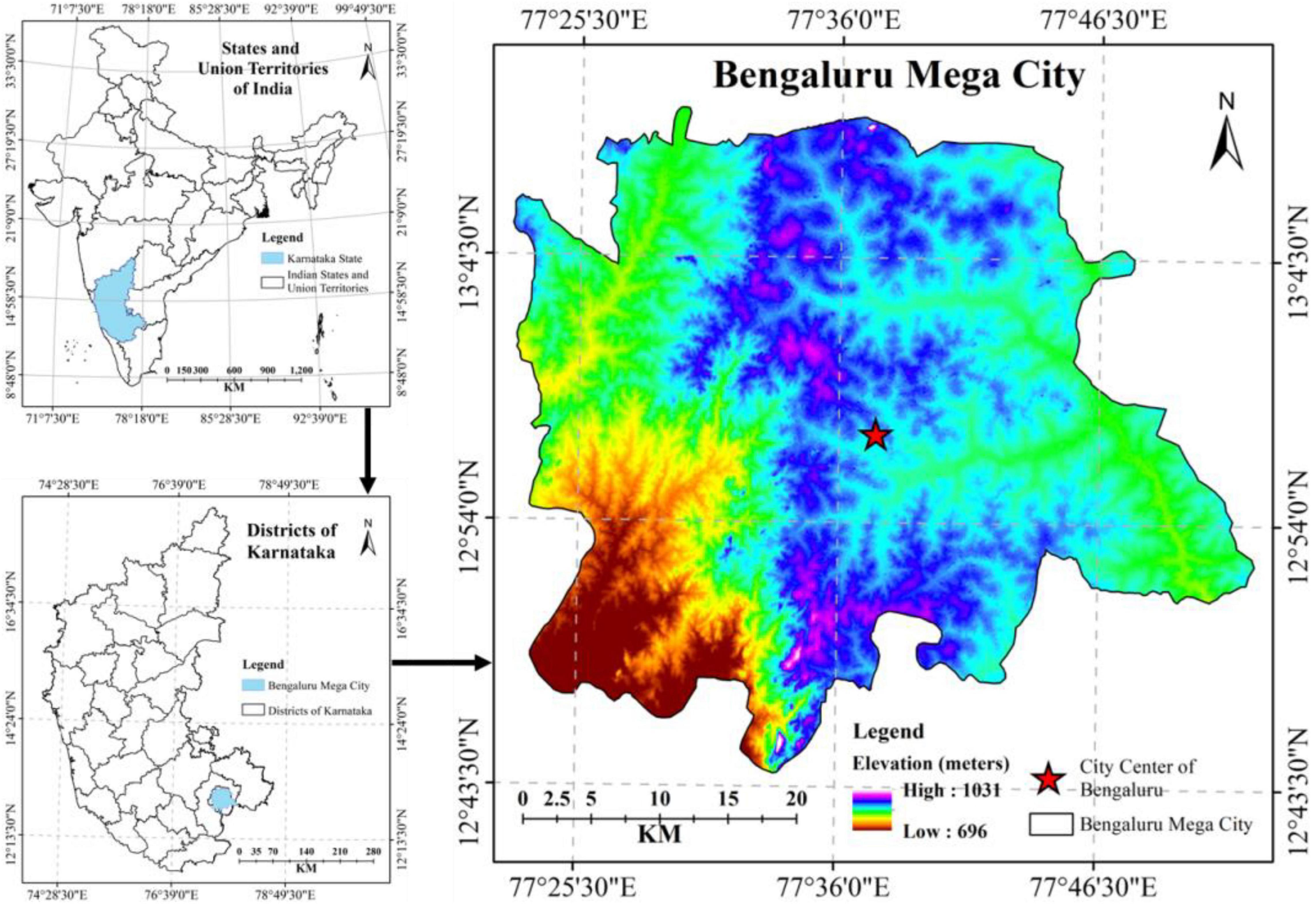
Figure 1. Study area, Bengaluru megacity.
The overall adopted methodology has been presented in Figure 2. We have explained the used methods in the following subheadings. First, we carried out LU/LC using a supervised approach where we selected the maximum likelihood classifier (MLC) algorithm to perform the classification based on the Anderson Classification Scheme, and this exercise has been done in ERDAS IMAGINE 2014 software. Later, we performed at-satellite brightness temperature on the Google Earth Engine (GEE) platform using Python codes (see Code S1 and Code S2 mentioned in the Supplementary File). All SUCI estimation and final output maps have been carried out using ArcGIS 10.3 software.
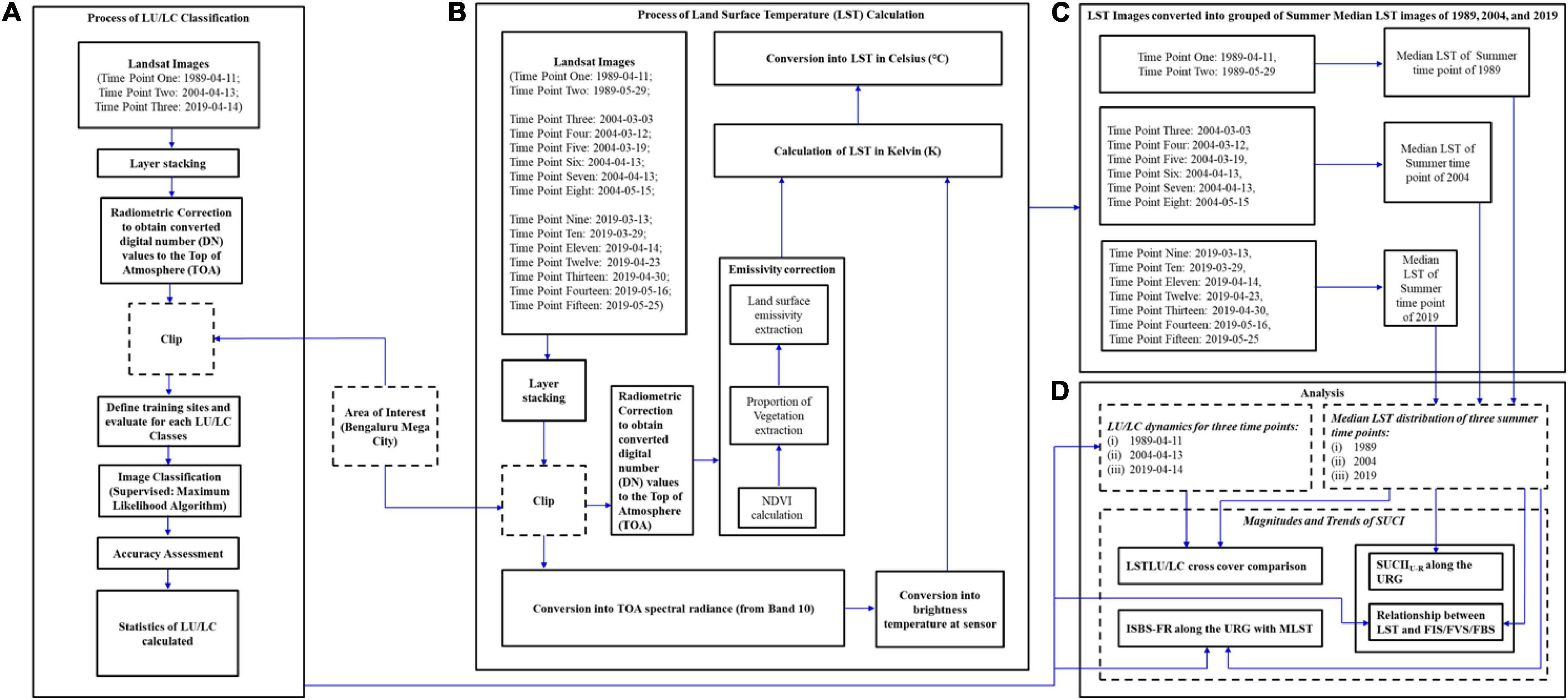
Figure 2. Flowchart of (A) LU/LC classification; (B) LST calculation; (C) median LST calculation for each summer timepoints of selected years (i.e., 1989, 2004, and 2019); and (D) analysis of the study.
For performing the LU/LC and SUCI dynamics, Landsat images were acquired in the summer dry season (March–May) in 1989, 2004, and 2019 (Table 1). GEE is used to estimate the summer median brightness temperatures (at–satellite) using thermal bands and the summer median best pixel for multispectral bands using preprocessed (atmospherically corrected) Landsat datasets. The incorporation of multiples images would create unambiguous output images to determine the patterns of LST in the summertime in the Bengaluru megacity. Based on previous studies (Ravanelli et al., 2018; Ranagalage et al., 2019), a similar technique is adopted to produce a median pixel in different areas that include several phases, as follows.
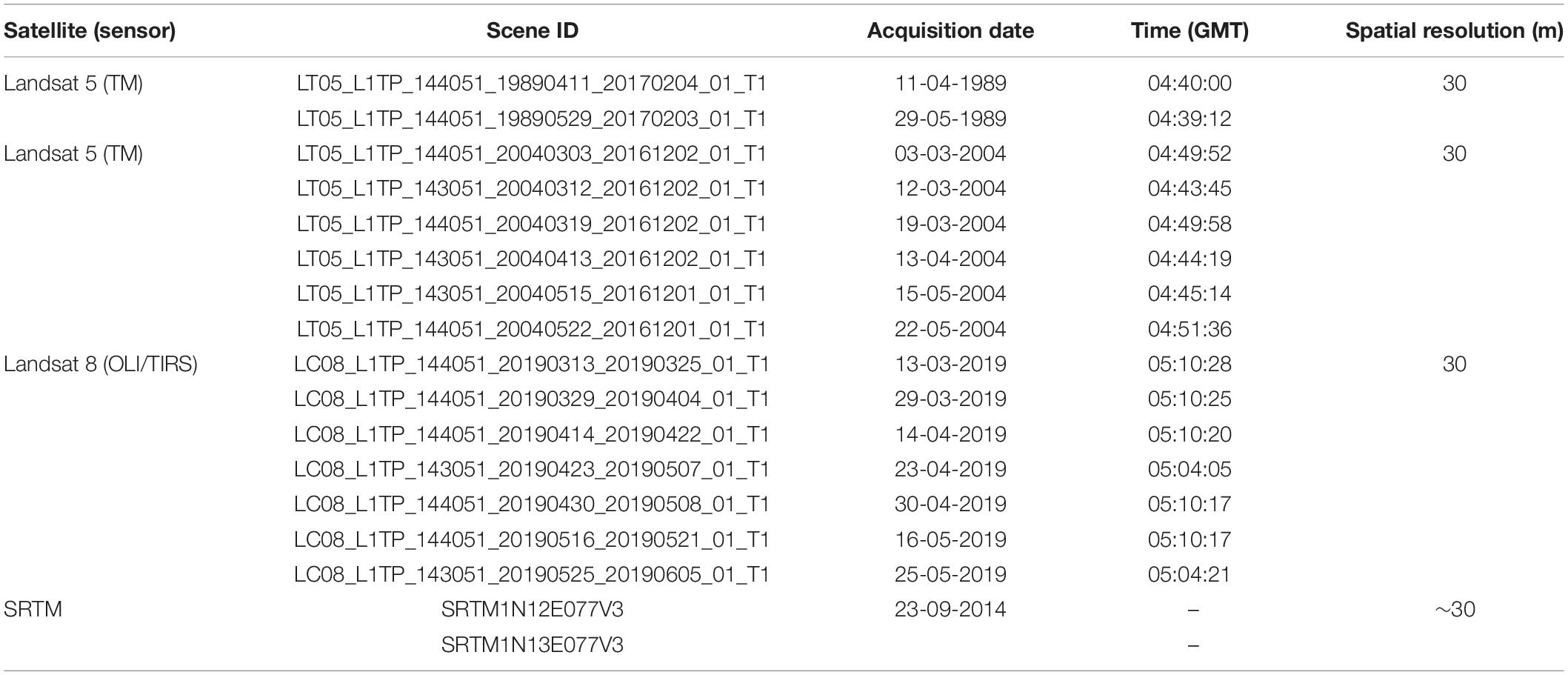
Table 1. Description of the Landsat datasets for the study area.
i. First of all, the boundary of the Bengaluru megacity has been imported and defined as an “Asset” in GEE. Subsequently, it has been used as a source of primary geometry in the whole executing process. Then, masking is done to overcome clouds in Landsat imageries.
ii. In GEE, the image collection tool has been used to produce the imagery for Bengaluru megacity for two summertime images of 1989 (Landsat 5), six images of 2004 (Landsat 5), and seven images of 2019 (Landsat 8 OLI/TIRS).
iii. Afterward, based on the median brightness temperatures (at–satellite), pixels have been extracted distinctly for 1989, 2004, and 2019 using the “ee.reducer” method in GEE (Ranagalage et al., 2019). The median value is taken to eliminate deficiency in LST calculation, so we can avoid the error caused due to very lower or higher spike pixels of LST values. The codes generated for this purpose have been attached in Supplementary Data (Google Earth Engine Code) as Code S1 for Landsat 5 (TM) and Code S2 for Landsat 8 (OLI/TIRS) for more details. Extracted median brightness temperatures (at–satellite) are used to calculate LST (°C) as described in section “Mapping of Land Use/Land Cover.” Having said this, we have used this median LST to present a raster LST presentation, and based on it, the MLST of the whole study area as well as each buffer zones area have been calculated in section “Impervious Surface–Bare Surface Fraction Ratio Along the Urban-Rural Gradient.”
iv. Finally, extracted images were projected in the WGS84/UTM 43N projection system.
To delineate LU/LC dynamics, three different timepoints satellite images of summertime, viz., 11 April 1989 [Landsat 5 (TM)], 13 April 2004 [Landsat 5 (TM)], and 14 April 2019 [Landsat 8 (OLI/TIRS)] of the Bengaluru megacity, were used (Table 1). For the generation of LU/LC maps, supervised classification based on Anderson’s classification scheme (Anderson et al., 1976) has been used where the MLC (Sarif and Gupta, 2021a,b, c) was chosen in ERDAS IMAGINE 2014 (Figure 2). Accordingly, the Bengaluru megacity was classified into five distinct LU/LC classes, namely agriculture land surface (AS) (crop and fallow fields), bare land surface (BS) (bare land, open land, sandy area, and open rocks), impervious land surface (IS) (urban area, rural area, road network, and parking lots), vegetation land surface (VS) (forest–steppe, tropical forests, and mixed forests), and water body surface (WS) (rivers, lakes, ponds, and scattered open water body). For performing the accuracy assessment for this classification, a sampling method called stratified random sampling has been executed. For this purpose, 250 points for all classes were chosen through visual interpretation for each class for all Landsat images (Ziaul and Pal, 2016; Rousta et al., 2018). Further, we partially compared and validated our LU/LC maps of 1989, 2004, and 2019 that had been partially compared and validated with the produced LU/LC maps of 1989, 2005, and 2017 by Govind and Ramesh (2019). Then, we carried out an accuracy assessment, i.e., user accuracy, producer accuracy, overall accuracy, and finally, Kappa coefficients, which have been calculated to find out the accuracy level in the performed classifications (Sexton et al., 2013; Ziaul and Pal, 2016; Sultana and Satyanarayana, 2018). Kappa coefficient is used to look out the level of agreement among the values of user-assigned and the values of predefined assigned and is called a nonparametric test. The accuracy test, viz., user, producer, overall, and Kappa coefficients were estimated for the above said timepoints using Equations 1–4, respectively.
where ψ states corrected classified pixels (CCP) (category), θ(ω) states classified pixels (CP) in that category [row total (RT)]; θ(ϕ) states CP in that category [column total (CT)]; γstates CCP (diagonal); β states classified reference pixels (CRP) in that category; N states total samples; τ states number of rows in error matrix; Xδ states total corrected samples in i-th row; Xς states RT; Xυ states CT.
For LST calculation, the thermal band raw data [Band 6 in Landsat TM using Equation 5 (Xiong et al., 2012; Pal and Ziaul, 2017), and Band 10 in Landsat 8 OLI/TIRS using Equation 6 (Sultana and Satyanarayana, 2020)] were converted into spectral radiance values:
where Lφ defines top of atmosphere (TOA) spectral radiance [watts/(m2 × sr × μm)], “gain” defines the multiplicative rescaling factor based on a specific band from the metadata, QCAL defines the values of digital number (DN) of quantized and calibrated pixel of the standard product, and “offset” defines the additive rescaling factor from a specific band from the metadata.
where QCALmin and QCALmax defines the minimum and maximum DN values of the images, respectively; Lmin and Lmax are the spectral radiance of TIR band at QCALmin and QCALmax, respectively. These rescaling factor values can be found in the metadata of Landsat images.
Then, the temperature value at the sensor (brightness) using Equation 7 was extracted (Avdan and Jovanovska, 2016; Bokaie et al., 2016; Ziaul and Pal, 2016; Rosa et al., 2017a; Estoque et al., 2018; Ranagalage et al., 2018b; Sultana and Satyanarayana, 2018):
where Tb defines brightness temperature (at sensor) in Kelvin; and K1 and K2 are the thermal conversion constants taken from the metadata (Band 6 for Landsat TM, and Band 10 for Landsat 8).
The extraction of LST (°C) (emissivity corrected images) has been performed using Equation 8 (Weng et al., 2004; Ranagalage et al., 2017; Sultana and Satyanarayana, 2020).
where λ states emitted radiance wavelength [11.5 μm for Band 6 (Weng et al., 2004) and 10.8 μm for Band 10 (Ranagalage et al., 2018a)]; ρ states h × c/σ (1.438 × 10⁻² m K), σ is Boltzmann constant (1.38 × 10⁻²³ J/K), h states Planck’s constant (6.626 × 10⁻³⁴ J × s), c as the velocity of light (2.998 × 10⁸ m/s), and ε states LSE, which has been estimated using the NDVI (Sobrino et al., 2004). The calculated LST value (Kelvin) was then converted to °C. The LST results, along with other climatic factors obtained in the present study, are compared and validated with NASA’s Prediction of Worldwide Energy Resource (POWER) project datasets available at https://power.larc.nasa.gov/data-access-viewer/, and a satisfactory level of similarity is observed at 12° 58′ 8.4″ latitude and 77° 34′ 37.92″ longitude.
The land surface emissivity (ε) was derived using Equation 9 (Sobrino et al., 2004).
In the above equation, m = (ε − ε) − (1 − εσ) Fεv and n = εs + (1 − εs) Fεv, where εs is the soil emissivity and εv is the vegetation emissivity. In this study, we have considered the result of Sobrino et al. (2004) and adopted m = 0.004 and n = 0.986. The proportion of vegetation (ρv) was estimated using the NDVI based on Equation 10 (Zhang et al., 2009).
where ρNIR refers to the surface reflectance values (SRV) of Bands 4 (Landsat 5 TM) and Band 5 [Landsat 8 (OLI/TIRS)] and ρRed refers to the SRV of Bands 3 (Landsat 5 TM) and Band 4 [Landsat 8 (OLI/TIRS)].
ρv has been estimated using Equation 11:
where NDVI refers to original NDVI values estimated using Equation 10, NDVImin refers to minimum NDVI value, and NDVImax refers to maximum NDVI values from respective images.
The LST intensity (LSTI) was calculated based on the URG zone from the city center (please see Figure 1 to find the city center location) (Stewart and Oke, 2009; Estoque and Murayama, 2017; Ranagalage et al., 2018a). Previous studies have shown that the 210 m buffer zone can be used to calculate the MLST and fraction of LU/LC (Estoque and Murayama, 2017; Ranagalage et al., 2018a,2019). One hundred twenty buffer zones were constructed in the analysis as this buffer size is best to extract the fraction values (Estoque et al., 2017; Ranagalage et al., 2017). Previously, URG analysis has been executed to extract the spatiotemporal variations in the environmental variables (Ranagalage et al., 2017, 2018a; Dissanayake et al., 2019b; Priyankara et al., 2019; Simwanda et al., 2019). The MLST of each buffer zone was carried out through zonal statistics, and FIS, FVS, and FBS were calculated in each buffer zone. The FIS, FVS, and FBS were calculated by considering the LU/LC of each buffer zone (Priyankara et al., 2019). The SUCI intensity (SUCII) based on the LU/LC categories (SUCIILU–LC) was calculated using the main LU/LC categories of each year. The main LU/LC categories, viz., AS, BS, IS, VS, and WS, were used to calculate the SUCII. The MLST of each LU/LC was extracted using zonal statistics available in ArcGIS 10.3.1. Hereafter, the MLST difference was calculated based on the MLST of each LU/LC (Estoque and Murayama, 2016, 2017; Ranagalage et al., 2018a,b; Rousta et al., 2018; Priyankara et al., 2019). The magnitude of SUCII based on URG (SUCIIU–R) was calculated based on Δ LST, Δ FIS, Δ FVS, and Δ FBS (Estoque and Murayama, 2017). The Δ LST, Δ FIS, Δ FVS, and Δ FBS of the Urban-Rural Zone (URZ1) were derived by subtracting URZs (URZ1 − URZ2… 120). The urban zone (UZ) was demarcated as the highest FIS, and the rural zone (RZ) was demarcated as the area with <10% of FIS from that of the city center (Estoque and Murayama, 2017; Ranagalage et al., 2018a). The magnitude of the LSTIU–R was calculated based on the Δ MLST, Δ FIS, Δ FVS, and Δ FBS following the methodology proposed by Estoque and Murayama (2017).
Ranagalage et al. (2018a) have introduced the green space – impervious surface fraction ratio and its intensity. We have proposed the ISBS–FR, and it was calculated by URZs using Equation 12 based on their procedure (Ranagalage et al., 2018a).
where, “FISz” (calculated using Equation 13) states IS fraction, and “FBSz” (calculated using Equation 14) states BS fraction in URZs (zones 1 to 120).
where “ISz” states the area of IS, “TAz” states the total area, and “BSz” states the area of BS in URZs (zones 1–120).
From the result of the accuracy assessment, user accuracy and producer accuracy were found to be more than 85 and 80%, respectively, while overall accuracy was found to be more than 85% in all-time points, i.e., 1989, 2004, and 2019. Kappa coefficient was found to be 0.836 in 1989, 0.847 in 2004, and 0.867 in 2019 (Table 2). This indicates the high reliability of various LU/LC maps generated in the present study.
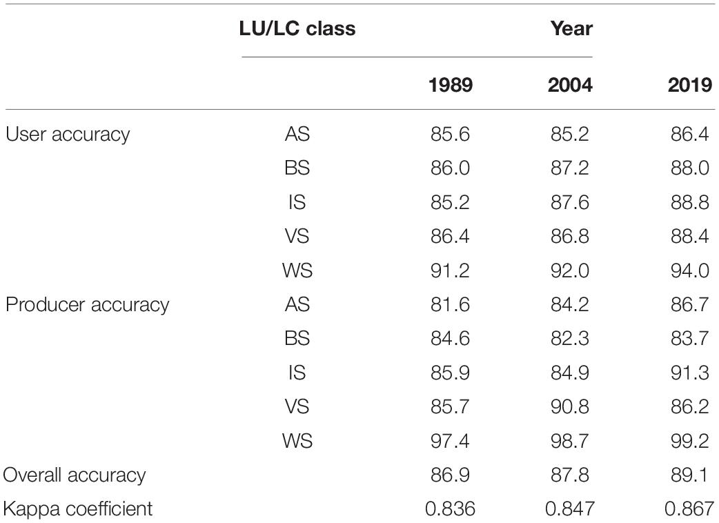
Table 2. Accuracy assessment report for LU/LC classification (1989–2019) for Bengaluru megacity.
The spatial distribution map of LU/LC is represented in Figure 3. Its area coverage is presented in Table 3 and its change coverage is in Table 4. IS has increased the most among all LU/LC classes from 1989 to 2019 by 344.4 km2 (20.99%), as it was 64.1 km2 (3.9%) in 1989, which increased to 150 km2 (9.1%) in 2004, and further increased to 408.5 km2 (24.9%) in 2019. VS has also increased from 1989 to 2019 by 11.9 km2 (0.8%), as in 1989, it was 95.9 km2 (5.8%) which increased, in 2004, to 145.2 km2 (8.9%), but it decreased in 2019 to 107.9 km2 (6.6%) although this was higher than in 1989. BS has continuously decreased the most among all LU/LC from 1989 to 2019 by 209.8 km2 (14%). BS was 1,213.5 km2 (74%), 1,088.0 km2 (66.3%), and 1,003.7 km2 (61.2%) in 1989, 2004, and 2019, respectively. AS has also decreased from 1989 to 2019 by 138.2 km2 (9.2%), and in 1989, it was 246.2 km2 (15%), which decreased in 2004 into 239.2 km2 (14.6%), and it further decreased in 2019 into 108.0 km2 (6.6%). WS has shown a decreasing trend from 1989 to 2019 by 8.3 km2 (0.6%) from 21.1 km2 (1.3%) in 1989 to 12.8 km2 (0.8%) in 2019.
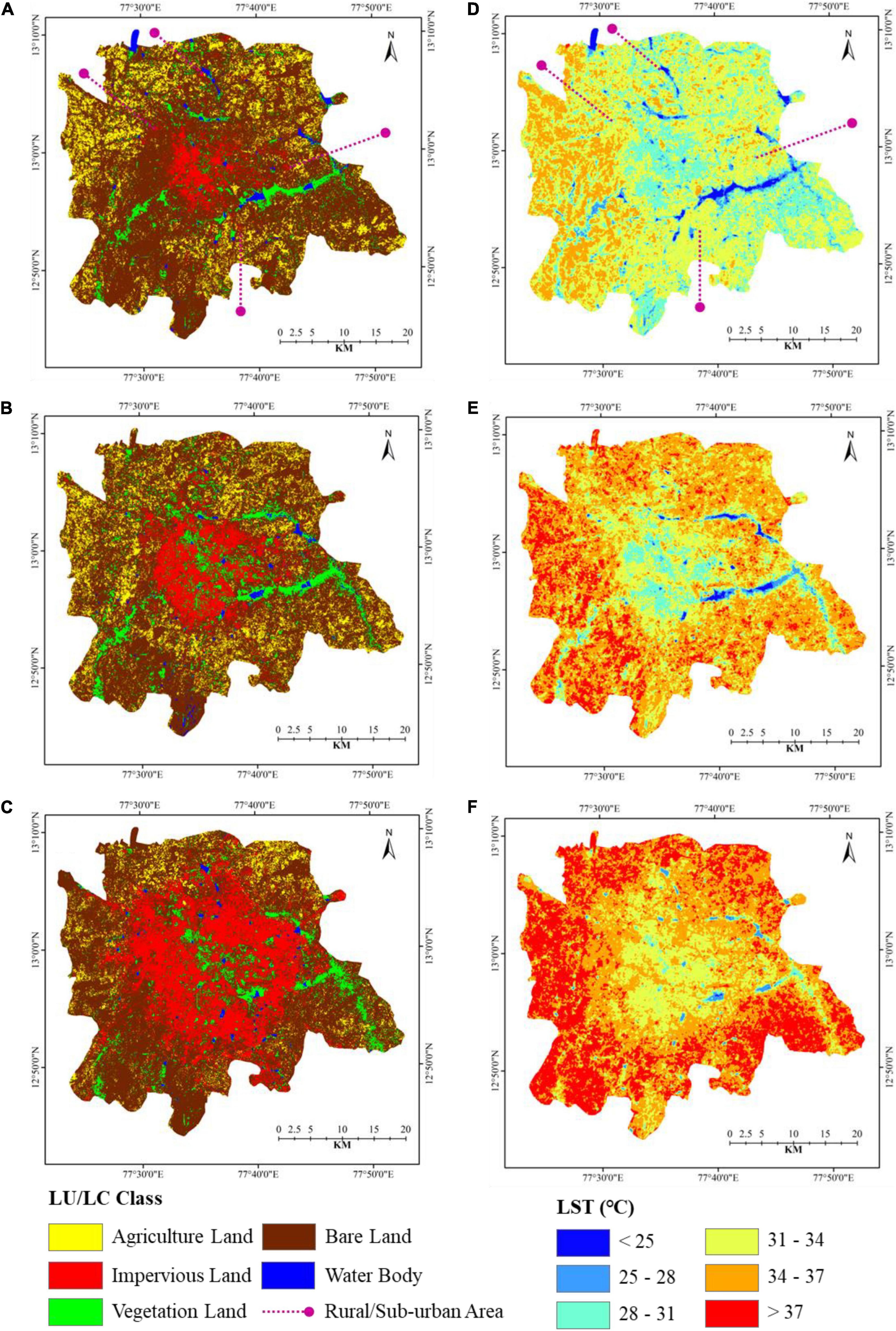
Figure 3. Land use/land cover maps and LST maps for depicting the spatial distribution of SUCI in Bengaluru megacity: (A) LU/LC in 1989; (B) LU/LC map in 2004; (C) LU/LC map in 2019; (D) median LST (°C) of summer timepoints in 1989; (E) median LST (°C) of summer timepoints in 2004; and (F) median LST (°C) of summer timepoints in 2019.
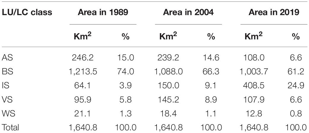
Table 3. Details of LU/LC change in Bengaluru megacity in 1989, 2004, and 2019.
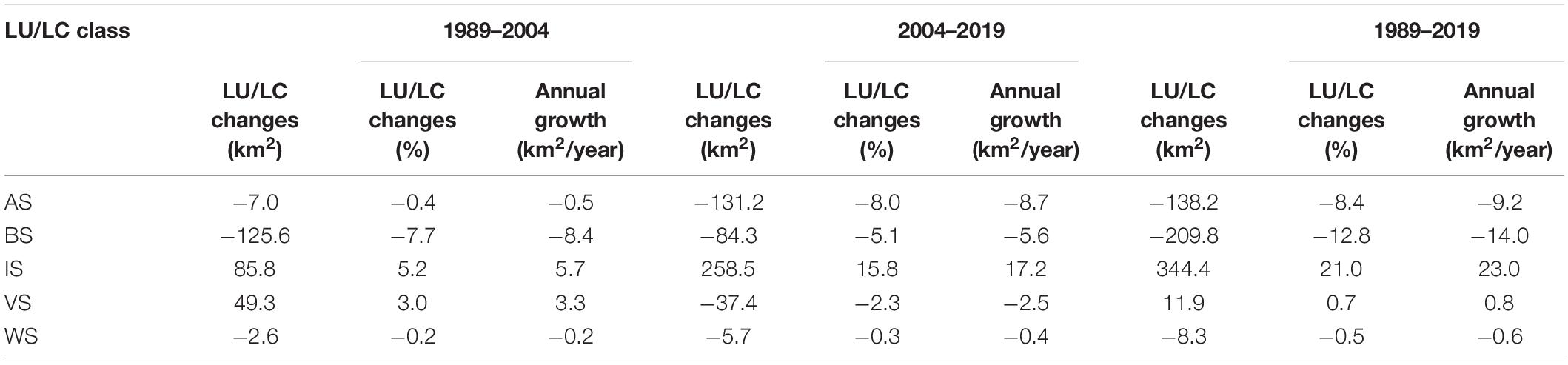
Table 4. Land use/land cover change 1989–2004, 2004–2019, and 1989–2019.
The map of the spatial distribution of SUCI is represented in Figure 3, where the summer season of three different years, i.e., 1989, 2004, and 2019, was selected to portray the spatiotemporal distribution of LST. In each year, more than one-time point based on available data was selected to better represent the LST distribution of the summer season, so we have calculated the median of LST of each summertime chosen point for each selected year, i.e., 1989, 2004, and 2019 (mentioned in section “Adopted Methodology”). We have further estimated the mean of each median LST for each selected summer season timepoint, and the result shows an increasing pattern of 32.52, 36.47, and 38.22°C in 1989, 2004, and 2019, respectively.
The MLST was lowest in the central part of the city whereas MLST was the highest in the outer/periphery of the city. The trend of MLST distribution is increasing from the city center toward the city periphery (Figure 3). The difference in MLST was nearly 5–8°C between the city center and the city’s periphery. This distribution pattern was called SUCI and observed in all three selected summertime points at 15 years of interval. This distribution pattern of MLST has been observed due to the presence of VS (patches of the forest, parks, grassland, etc.) and WS (small-large size of ponds/lakes) in considerable amount in the central part of the city while the presence of IS (built-up or, concrete type), AS (fallow and/or abandoned type), and BS (bare and/or sandy type) is observed in a remarkable amount in the periphery of the city.
During the summer in 1989 (Figure 2), the central part of the city, such as Chickpet, Malleshwaram, and Sulthangunta, experienced MLST of 23–30°C, while suburban/rural/city’s periphery areas such as Makali (in the north–west), Seegehalli (in the west), Bannerughatta, and Bommasandra (in the south) have experienced MLST of 30–35°C. Thus, it showed a higher mean in suburban/rural areas than in the city center, with a difference in urban–rural MLST of 7–12°C (Figure 3). Later, in the summer of 2004, the same central part of the city experienced MLST of 25–32°C whereas the same suburban/rural/city’s periphery area experienced MLST of 33–37°C, hence, so forth, the observed difference of MLST between urban and rural area was 8–12°C. Finally, during the summer of 2019, the same central part of the city experienced MLST of 28–34°C, whereas the same suburban/rural/city’s periphery area experienced MLST of 34–40°C, leading to a 6–12°C MLST difference between urban and rural area.
Table 5A shows the MLST of the LU/LC categories in three selected time points, i.e., 1989, 2004, and 2019. The MLST of each LU/LC category showed an increasing pattern from 1989 to 2019. However, the lowest increasing patterns are shown in the IS category as 4.5°C, while the highest recorded in AS is 5.5°C. Table 5B shows the magnitude of MLST in the main LU/LC categories from 1989 to 2019. It is observed that the magnitude of MLST between IS and VS shows a decreasing pattern of 2.7 to 2.3°C while showing an increasing pattern among IS and BS from 0.9 to 1.5°C from 1989 to 2019. A similar pattern is observed between IS and AS. It shows an increasing pattern of the magnitude of MLST as 2°C in 1989 and 3°C in 2019. The highest MLST difference can be seen among VS and AS each year.
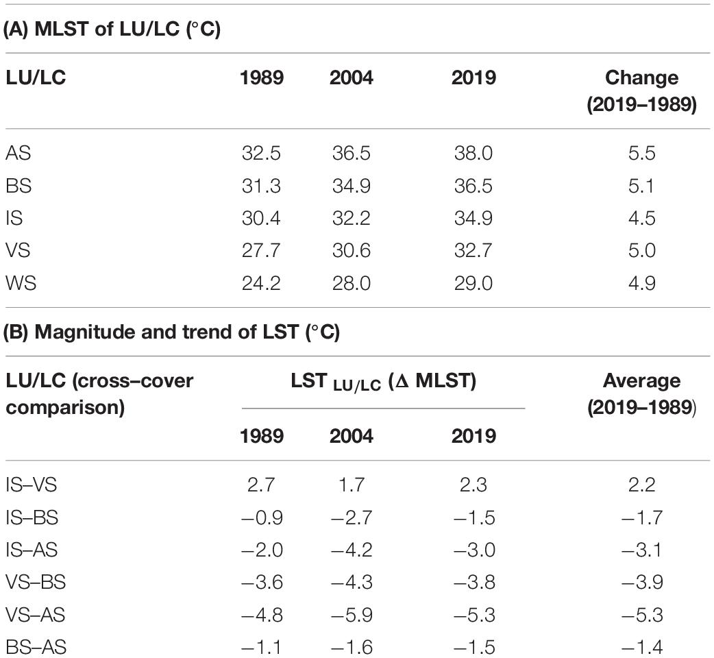
Table 5. Mean LST of LU/LC and their magnitude and trend of SUCIIIS–GS (°C).
The SUCII has shown the interrelationship among MLST and FIS, FVS, and FBS over URG in three different timepoints, i.e., 1989, 2004, and 2019 (Figure 4A). The urban–rural space has been differentiated using a FIS (with <10% of fraction IS as threshold value). In the summer timepoints of 1989, from the city center grid to 29 zones (∼6.09 km), it was observed that the average MLST was 30°C while FVS was 6.5%, FIS was 34.9%, and FBS was 57.1%. After 29 zones, the average MLST observed was 31.1°C till 120 zones (∼25.2 km), while FVS, FIS, and FBS were 6.2, 1.4, and 76.3%, respectively. Thus, it is evident that, after 6.09 km from the city center, the MLST has increased by 1.1°C over the suburban/rural area till 25.2 km, whereas the FVS has declined by 0.4%, but FBS has inclined by 19.3% (Figure 4B). In the summer timepoints of 2004, the city center formed a grid at 46 zones (∼9.66 km), and it was observed that the MLST was 32.1°C while FVS was 16.8%, FIS was 38.4%, and FBS was 40.7%. Whereas after 46 zones, the MLST observed was 34.8°C till 120 grids (∼25.2 km) while FVS was 8.2%, FIS was 1.6%, and FBS was 72.5%. Thus, it is evident that after 9.66 km from the city center, the MLST has increased by 2.7°C over the suburban/rural area till 25.2 km, whereas the FVS has drastically declined by 8.6%, but FBS has inclined by 31.8% (Figure 4C). In the summer timepoints of 2019, the city center formed a grid at 74 zones (∼15.54 km), and it has been observed that the average MLST was 34.1°C while FVS was 9.8%, FIS was 43.5%, and FBS was 43.3%. After 74 zones, the average MLST observed was 35.9°C to 120 zones (∼25.2 km), while FVS was 8.2%, FIS was 4.6%, and FBS was 78.2%. It is evident that after 15.54 km from the city center, the MLST has increased by 1.8°C over the suburban/rural area till 25.2 km, whereas the FVS has drastically declined by 1.6%, but FBS has inclined significantly by 34.9% (Figure 4D).
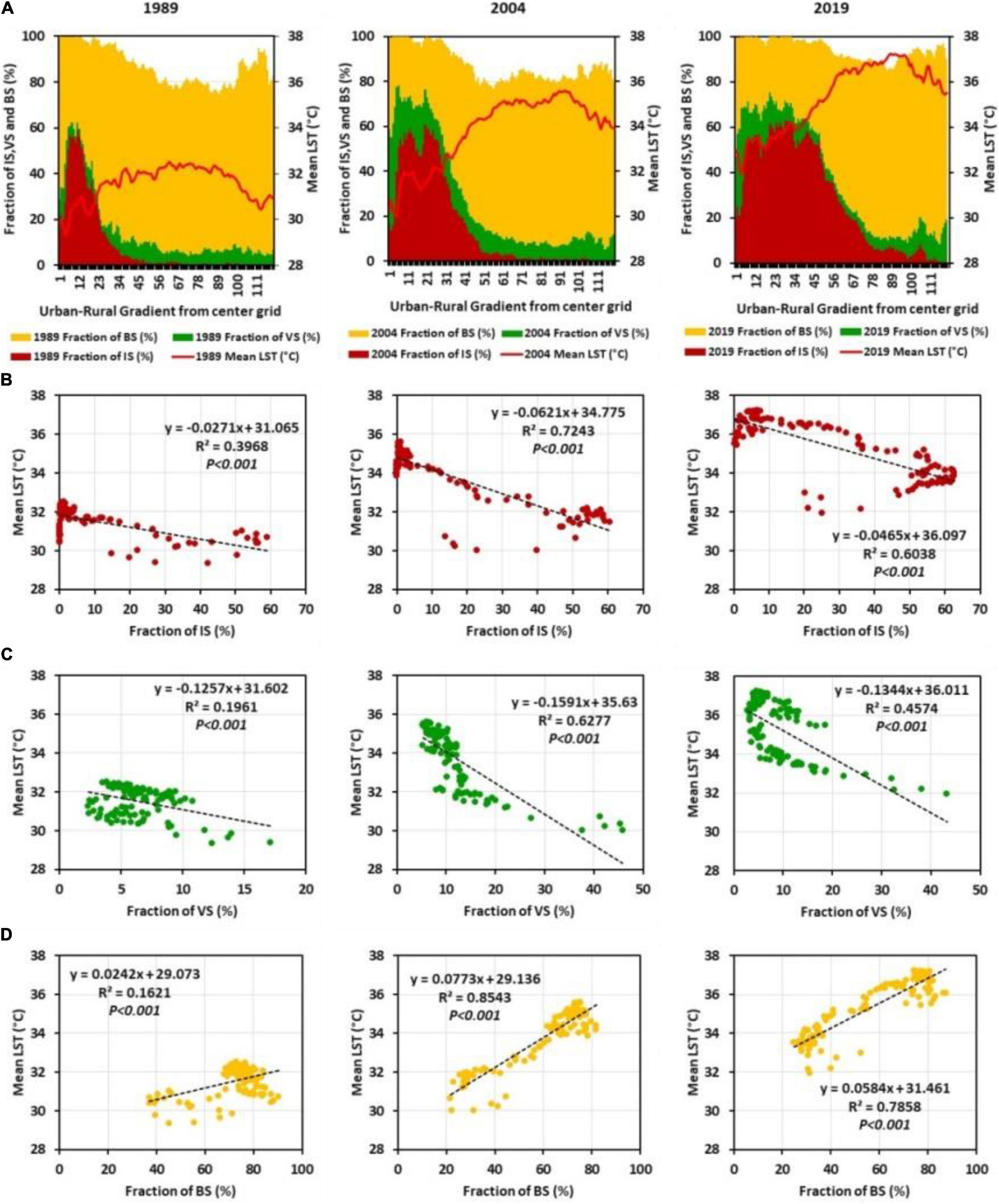
Figure 4. (A) Spatial pattern of MLST, FIS, FVS, and FBS along the URG for 1989, 2004, and 2019; (B) scatter plots between MLST and FIS, (C) scatter plots between MLST and FVS, and (D) scatter plots between MLST and FBS.
The relationship among MLST and FIS has been found negative with a statistical significance of p < 0.001 in all-timepoints of 1989 (R2 = 0.40), 2004 (R2 = 0.72), and 2019 (R2 = 0.60) (Figure 4B). The same findings were also observed in Bengaluru megacity by Siddiqui et al. (2021), where the correlation coefficient among MLST and FIS was negative in both selected timepoints of January 2019 (R2 = 0.85) and April 2019 (R2 = 0.94). The relationship among MLST and FVS has also been found negative with statistical significance of p < 0.001 in all-timepoints of 1989 (R2 = 0.20), 2004 (R2 = 0.63), and 2019 (R2 = 0.46) (Figure 4C), but the relationship among MLST and FBS has been found positive with statistical significance of p < 0.001 in all-timepoints of 1989 (R2 = 0.16), 2004 (R2 = 0.85), and 2019 (R2 = 0.79) (Figure 4D). This pattern of lower concentration of MLST in the central part of the city than in suburban/rural areas is because of the higher presence of vegetation and water bodies in the central part of the city than in the suburban/rural area. This trend led to the constitution of the SUCI phenomena in the study area.
Figure 5A shows the magnitude of Δ MLST, Δ FIS, Δ FVS, and Δ FBS along URZ. As stated earlier, the zone of urban–rural space from the city center to the city periphery has been identified by considering <10% of fraction IS as the threshold value. Based on this, the rural zone as URZ29 (after the city center of 6.09 km) in 1989 moved away to URZ46 (after the city center of 9.66 km) in 2004, and it again moved away to URZ74 (after the city center of 15.54 km) in 2019. The magnitude of SUCIIU–R was carried out based on the demarcated space of URZs. As per the demarcated space, the temperature difference was 1.92°C in 1989, 4.61°C in 2004, and 2.66°C in 2019.
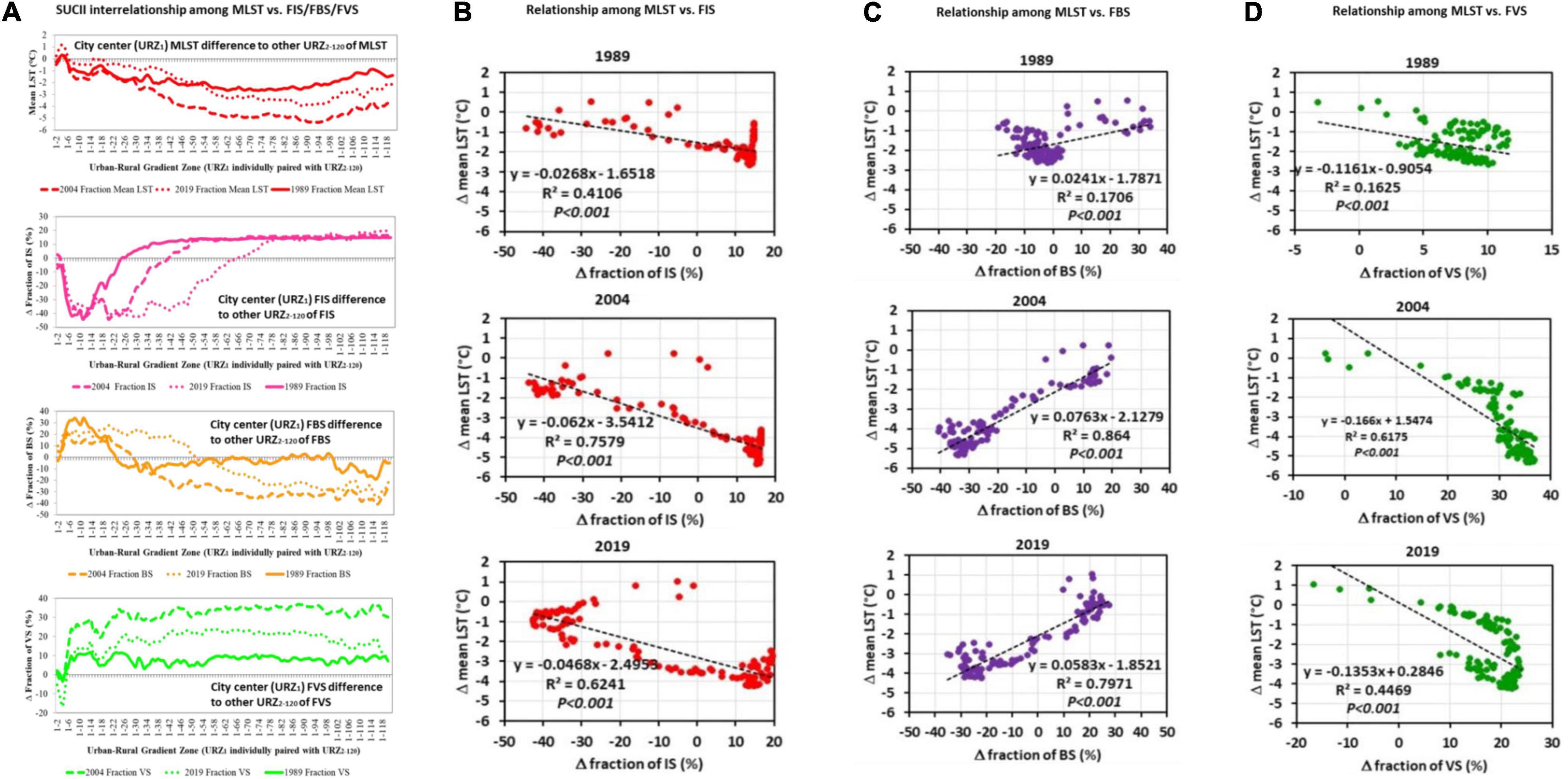
Figure 5. Magnitude of the trend of SUCIIU–R (°C), FIS, FVS, and FBS along the URZ and their relationship; (A) the difference of MLST, FIS, FVS, and FBS of URZ1 along the MLST, FIS, FVS, and FBS of URZ2–120 extractions for the trend of SUCIIU–R (°C) depiction; (B) relationship of the magnitude of MLST and FVS; (C) relationship of the magnitude of MLST and FBS; and (D) relationship of the magnitude of MLST and FVS.
Figure 5B shows the relationship among the magnitude of Δ MLST vs Δ FIS along URZs (zones 1–120) where the city center (zone 1) has been compared with the rest of the other zones. In all–time points, i.e., 1989, 2004, and 2019, a negative trend has been observed with R2 values of 0.41, 0.76, and 0.62, respectively, portraying that the city center (up to zone 29 for 1989, zone 46 for 2004, and zone 74 for 2019) has higher growth of built-up land as compared to the rest of the zones.
Figure 5C shows the relationship among the magnitude of Δ MLST vs Δ FVS along URZs (zones 1–120) where the city center (zone 1) has been compared with the rest of the other zones. The relationship has observed a negative trend with R2 values of 0.16, 0.62, and 0.45 in all the three-time points of 1989, 2004, and 2019, respectively. This reflects that the city center has higher growth of FIS in all-time points compared to the rest of the zones in comparing the time point of 1989 (zone 1) to other time points of 2004 and 2019 in suburban/rural areas (zone 120).
Figure 5D shows the relationship among the magnitude of Δ MLST vs Δ FBS along URZ (UR) where the city center (zone 1) has been compared with the rest of the other zones. In all-time points, i.e., 1989, 2004, and 2019, the relationship has been found positive with R2 values of 0.17, 0.86, and 0.80, respectively, which portray that the city center (zone 1) has lower growth of bare land compared to rest of the zones to suburban/rural area (zone 120) in all-time points.
In this section, the ratio of ISBS fraction along with MLST is analyzed (Figure 6A). The ratio of ISBS fraction has expanded after 1989 from the city center towards its periphery along with MLST. In 1989, the ISBS–FR was highly concentrated in the range of center zone to 25 zones with an ISBS–FR of 0.25–1.6, and the MLST was 28.5–30.5°C. However, the ISBS–FR dropped sharply after 25 zones, and the ratio was found in the range of 0–0.05 to 120 zones, whereas the MLST pattern hiked after 25 zones up to 31.5°C and fell at 110 zones with 30°C. In 2004, both the ISBS–FR and MLST expanded in comparison to 1989 as the ISBS–FR was highly concentrated in the range of center zone to 35 zones with an ISBS–FR of 0.35–2.6, and the MLST was 30.5–32°C but the ISBS–FR dropped (sharply fallen after 35 girds and ratio found in the range of 0–0.05 till 120 zones), whereas the MLST pattern hiked after 35 zones (up to 35.5°C and fallen at 110 zones with 34°C). In 2019, again, both the ISBS–FR and MLST had expanded in comparison to 2004 as the ISBS–FR was highly concentrated in the range of center grid to 50 zones with an ISBS–FR of approximately 0.4–2.5, and the MLST was approximately 31.5–34.5°C. Further, the ISBS–FR dropped sharply fallen after 55 zones, and the ratio was in the range of 0.05–0.6 till 120 zones, whereas the MLST pattern hiked after 55 zones (up to 36.5°C and fell at 118 zones with 35°C).
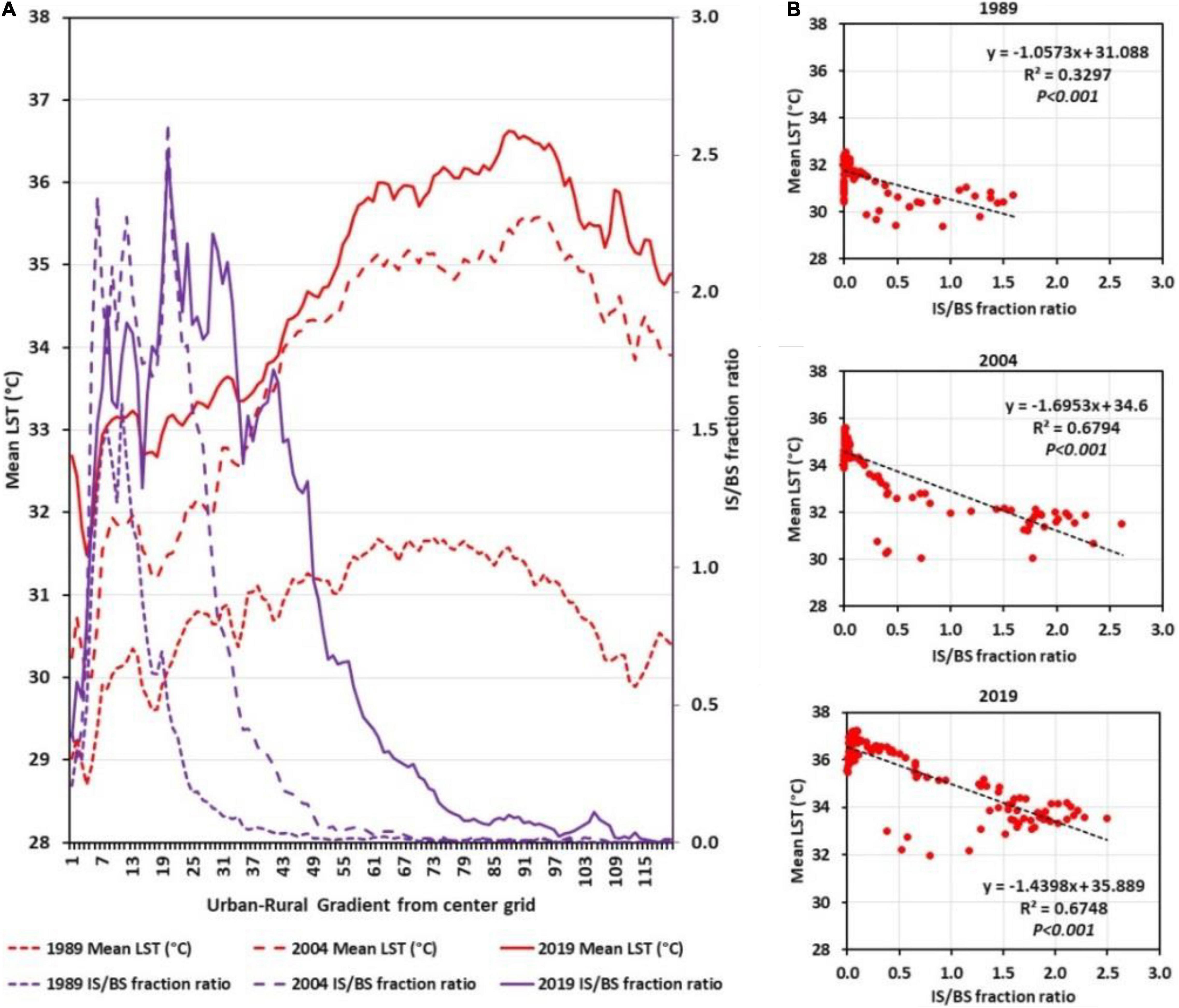
Figure 6. (A) Spatial pattern of the MLST, ISBS–FR along the URG; and (B) scatter plots between MLST and the ISBS–FS.
It also deals with the interrelationship among the ISBS–FR and means of LST (Figure 6B). Negative relationship is observed in all three time points, i.e., 1989 (R2 = 0.33), 2004 (R2 = 0.68), and 2019 (R2 = 0.67). The ISBS–FR increased in the city center and decreased in the city periphery, whereas MLST decreased in the city center and increased in the city periphery. Therefore, due to the increasing ISBS–FR pattern, there is a decreasing pattern in MLST in the city center and vice versa on the city periphery, leading to UCI phenomena in the Bengaluru megacity.
Urbanization is the source of economic and social prosperity for its people, but it has severe environmental consequences (Estoque and Murayama, 2014, 2016). The Bengaluru megacity has undergone high development of impervious land, especially from 1989 to 2019, by 344.4 km2 (20.99%) (Tables 2, 3). There are numerous urban patches in the central part of the city that have increased in all the periods, i.e., 1989–2004, 2004–2019, and 1989–2019 (Figure 3 and Table 4). Due to the process of urbanization, rapid depletion has been seen in the WS and AS at a very remarkable rate. Although VS increased by 49.3 km2 from 1989 to 2004, mostly in the central part of the city, it decreased by 37.4 km2 in 2004–2019. Most of the impervious development has occurred in the north, north-west, east, south, and south-west at a rapid rate. The same pattern was observed by Govind and Ramesh (2019). This process of expansion in IS led to the intensification of LST in all the three-time points. In all periods, IS has experienced higher LST than VS and WS remarkably (Table 5). This pattern has also been observed in previous studies of other researchers (Estoque et al., 2017; Ranagalage et al., 2018a; Rousta et al., 2018). The central part of the city has witnessed lower MLST distribution than the periphery of the city due to (a) the city’s climate being of the semi–arid type (Govind and Ramesh, 2019), (b) more than 50% of the area of AS being in an open condition, which means that the agricultural field is abandoned at that particular time due to seasonal cropping activity exhibiting higher albedo, (c) the outer space of the city being mainly covered with bare soil, and bare rocks of the city being located on Mysore Plateau, and (d) the city having numerous lakes and water bodies with scattered distributed vegetation patches of small–large scales in the central part.
The rapid urbanization from the city center toward the city’s periphery of the Bengaluru megacity has great effects on the increasing pattern of SUCI magnitude. The lower MLST concentration has been observed in VS and WS as compared to IS, BS, and AS at a great scale by 2.7–8.3°C in 1989, 1.7–8.5°C in 2004, and 2.3–9°C in 2019 (Table 5). This indicates that vegetation and water have a very prominent role in reducing the LST distribution on the landscape of the Bengaluru megacity. A similar pattern of LST over LU/LC classes has been observed in the Eliya, Nuwara, and Kandy cities of Sri Lanka (Ranagalage et al., 2018a,2019; Dissanayake et al., 2019c), Tehran city of Iran (Rousta et al., 2018), and Baguio City in the Philippines (Estoque and Murayama, 2017; Figure 7). It has been observed that from the city center to the periphery of the city, the trend of LST has been enlarged, reflecting that the core city has experienced lower LST than the city periphery in all three–time points of 1989, 2004, and 2019. The results indicate that the pattern of UCI has been the same at each time interval, but the LST has expanded greatly from its previous time point (Figure 6).
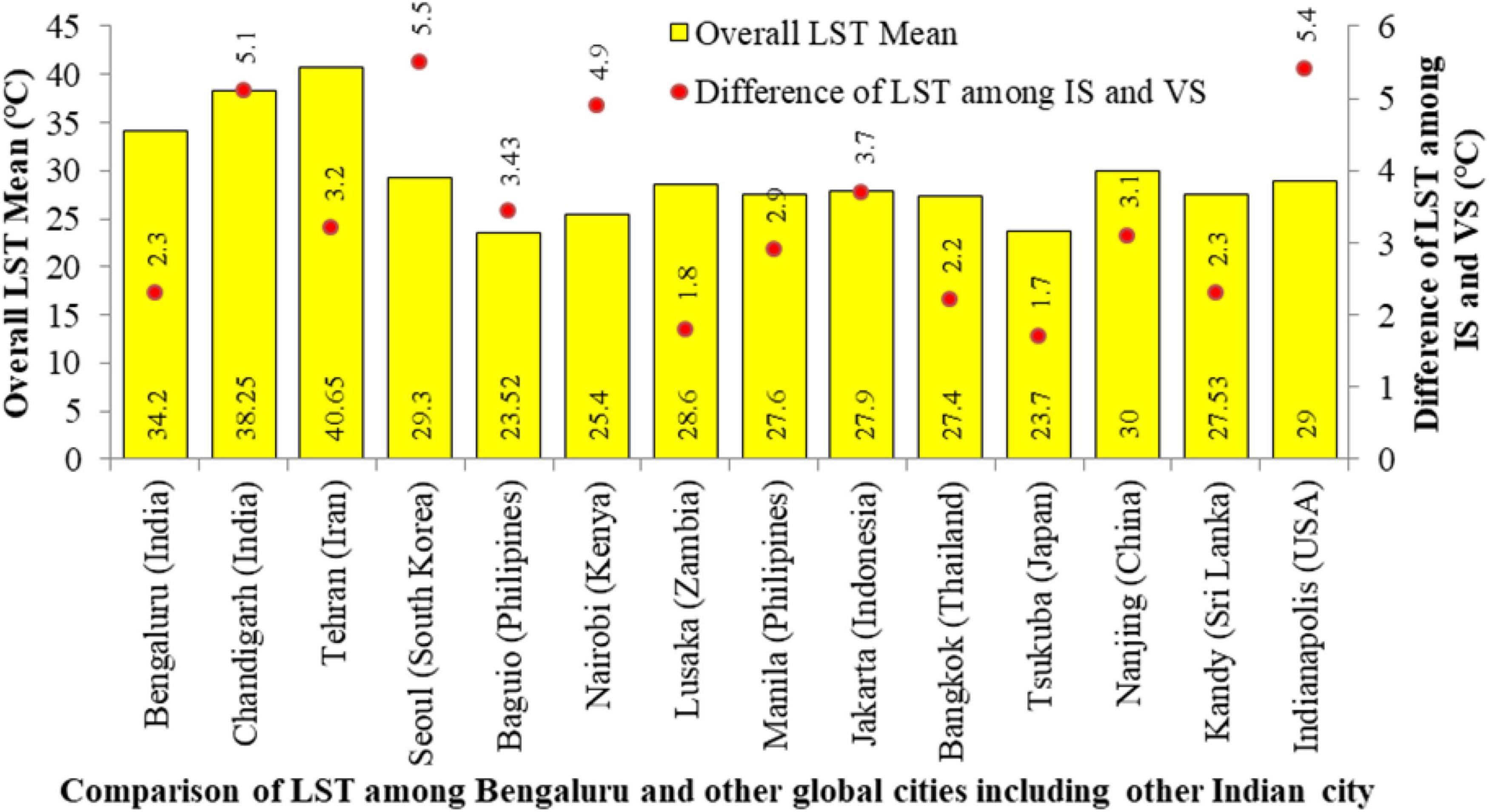
Figure 7. Comparison of overall LST mean and difference of LST mean among IS and VS between Bengaluru and other global cities (including other Indian cities) (Liu and Weng, 2008; Kong et al., 2014; Estoque et al., 2017; Estoque and Murayama, 2017; Ranagalage et al., 2018a,b; Rousta et al., 2018; Priyankara et al., 2019; Simwanda et al., 2019; Sultana and Satyanarayana, 2020).
Therefore, it is a significant matter of concern to address the enlargement of the SUCI phenomena due to the expansion of impervious land at a large scale in all-time points of 1989, 2004, and 2019. This has happened due to the explosive demands of the population for their needs for residential, commercial, industrial, and road networks. As the UN has said that this megacity population was 3.90 million in 1989, which drastically increased to 11.88 million, and if the trend remains the same, then the population of this megacity will be 18.07 million in 2035 (Figure 8). These population trends indicate that this megacity is going to face huge pressure on its natural resources shortly. This altogether will lead to a critical situation in the local environment of the city, thereby gradually degrading the standard of living life. Therefore, it is essential to mitigate its effects as early as possible before the time is over for the corrective measures. Some of the possible strategies that could be adopted include the use of tree plantation, green and cool roof creation, light material and light color paints, water body creation at small to big sizes, evaporative and water retentive pavements, and water–retaining pavements (Mohajerani et al., 2017; Rosa et al., 2017b). As per the IPCC (2019) report, it is said that small to large-scale landscape monitoring needs to be incorporated into planning and policymaking to reduce the severe effects of climate change on humans, including animals, flora, and fauna). Hence, it is essential to adopt strategies to mitigate and reduce the enlargement of SUCI effects. It is also very much required to monitor the spatial development of the city to prevent the creation of a highly critical situation in the context of resource conservation and environmental sustainability.

Figure 8. Population of Bengaluru megacity.
The present study has been executed in the GEE platform, which enabled us to carry out our result of LST for Bengaluru, one of the largest megacities of India and even in Southeast Asia. The results of LST have been represented at multiple time points during the summer season (March–May) in selected years (i.e., 1989, 2004, and 2019), which enhanced the trend of the spatial distribution of LST. This study depicts the Bengaluru megacity and its neighboring areas, which were much swayed by the formation of SUCI from 1989 to 2019. Based on the zones of URG analysis, we have focused on differentiating the urban and rural areas based on FIS that is extracted from LU/LC dynamics. It has been found that the magnitude of Δ MLST was 2.05°C in 1989, which increased to 4.65°C in 2004, and later, it became 3.20°C in 2019, which was more as compared to 1989 but was less as compared to 2004. This was the trend that has been focused on understanding the LST fluctuation. This witnessing trend of SUCII has been dramatically affected by the impervious development of the Bengaluru megacity. The result of cross cover comparison depicts Δ MLST of IS was higher than Δ MLST of WS and Δ MLST of VS at all-time points in 1989, 2004, and 2019. This indicates that IS has a more significant role in the intensification of LST than WS and VS, or in other words, it also indicates that WS and VS have a very prominent role in reducing the LST intensity than IS as well as other LU/LC classes.
The pattern of urbanization has enlarged and shifted URZ25 (5.25 km) to URZ55 (11.55 km) with FIS (%) 9.3 to 28.6 from 1989 to 2019, respectively. In addition, the results have also found that the FVS (%) increased from 6.3 to 9.2 from 1989 to 2019, although it was higher in 2004 with 11.5 but decreased in 2019. The ISBS–FR can be used as an indicator for the delineation of the formation of SUCI in the city. Urban planners and policymakers should pay attention to the utilization of ISBS–FR for reducing the adverse effects of SUCI. The expansion of vegetation space and water bodies in small to big sizes is one of the best ways to minimize the thermal status of the environment of the Bengaluru megacity. The result can help in the identification of spatial SUCI formation in the city. This study recommends that the spreading vegetation space and maximizing water bodies of different sizes have an immediate effect on maintaining the thermal standard of living life in the Bengaluru megacity. Otherwise, the impervious development takes its own course to intensify the SUCI effects, which could be more dangerous for the environmental sustainability of the city. The findings of the present research can be considered as an indicator of landscape planning or urban planning for the Bengaluru megacity of India.
However, the present study faced limitations due to the use of freely available RS datasets, and therefore, the authors recommend the use of fine spatial resolution data (preferably 1 m) and high temporal resolution data (preferably daily or alternative day) for delineation of the landscape information, e.g., LU/LC classification and LST computation, with explicit clarity for sustainable development of the Bengaluru megacity.
The datasets presented in this article are not readily available because its personal property as it has been produced by our research team. So, we cannot share it publically. Requests to access the datasets should be directed to MS.
MS and MR introduced the topic and directed the data processing, analysis, and writing of the manuscript. RG and YM assisted in the research design and writing the manuscript. All authors contributed to the article and approved the submitted version.
This research was partly supported by the Japan Society for the Promotion of Science (JSPS) grants of 21K01027 and 18H00763.
The authors declare that the research was conducted in the absence of any commercial or financial relationships that could be construed as a potential conflict of interest.
All claims expressed in this article are solely those of the authors and do not necessarily represent those of their affiliated organizations, or those of the publisher, the editors and the reviewers. Any product that may be evaluated in this article, or claim that may be made by its manufacturer, is not guaranteed or endorsed by the publisher.
We are grateful to United States Geological Survey (USGS) for providing the Landsat data for this study.
The Supplementary Material for this article can be found online at: https://www.frontiersin.org/articles/10.3389/fevo.2022.901156/full#supplementary-material
Anderson, J. R., Hardy, E. E., Roach, J. T., and Witmer, R. E. (1976). “A land use and land cover classification system for use with remote sensor data,” in A Revision of the Land Use Classification System as Presented in, 671, (Washington: U.S. Geological Survey Circular).
Avdan, U., and Jovanovska, G. (2016). Algorithm for automated mapping of land surface temperature using landsat 8 tatellite data. J. Sens. 2016, 1–8. doi: 10.1155/2016/1480307
Bokaie, M., Zarkesh, M. K., Arasteh, P. D., and Hosseini, A. (2016). Assessment of urban heat island based on the relationship between land surface temperature and land use/land cover in Tehran. Sustain. Cities Soc. 23, 94–104. doi: 10.1016/j.scs.2016.03.009
Chakraraborty, S. D., Kant, Y., and Mitra, D. (2015). Assessment of land surface temperature and heat fluxes over Delhi using remote sensing data. J. Environ. Manage. 148, 143–152. doi: 10.1016/j.jenvman.2013.11.034
Chaudhuri, A. S., Singh, P., and Rai, S. C. (2018). Modelling LULC change dynamics and its impact on environment and water security: geospatial technology based assessment. Ecol. Environ. Conserv. 24, 300–306.
Dissanayake, D., Morimoto, T., Murayama, Y., and Ranagalage, M. (2019a). Impact of landscape structure on the variation of land surface temperature in sub-saharan region: a case study of addis ababa using landsat data. Sustainability 11:2257. doi: 10.3390/su11082257
Dissanayake, D., Morimoto, T., Ranagalage, M., and Murayama, Y. (2019b). Impact of urban surface characteristics and socio-economic variables on the spatial variation of land surface temperature in lagos city, nigeria. Sustainability 11:25. doi: 10.3390/su11010025
Dissanayake, D., Morimoto, T., Ranagalage, M., and Murayama, Y. (2019c). Land-use/land-cover changes and their impact on surface urban heat islands: case study of kandy city. Sri Lanka. Climate 7:99. doi: 10.3390/cli7080099
Estoque, R. C., and Murayama, Y. (2014). Measuring sustainability based upon various perspectives: a case study of a hill station in Southeast Asia. Ambio 43, 943–956. doi: 10.1007/s13280-014-0498-7
Estoque, R. C., and Murayama, Y. (2016). Quantifying landscape pattern and ecosystem service value changes in four rapidly urbanizing hill stations of Southeast Asia. Landsc. Ecol. 31, 1481–1507. doi: 10.1007/s10980-016-0341-6
Estoque, R. C., and Murayama, Y. (2017). Monitoring surface urban heat island formation in a tropical mountain city using Landsat data (1987–2015). ISPRS J. Photogramm. Remote Sens. 133, 18–29. doi: 10.1016/j.isprsjprs.2017.09.008
Estoque, R. C., Murayama, Y., and Myint, S. W. (2017). Effects of landscape composition and pattern on land surface temperature: an urban heat island study in the megacities of Southeast Asia. Sci. Total Environ. 577, 349–359. doi: 10.1016/j.scitotenv.2016.10.195
Estoque, R. C., Pontius, R. G., Murayama, Y., Hou, H., Thapa, R. B., Lasco, R. D., et al. (2018). Simultaneous comparison and assessment of eight remotely sensed maps of Philippine forests. Int. J. Appl. Earth Obs. Geoinf. 67, 123–134. doi: 10.1016/j.jag.2017.10.008
Frey, C. M., Rigo, G., and Parlow, E. (2005). “Investigation of the daily urban cooling island (UCI) in two coastal cities in an arid environment: Dubai and Abu Dhabi (U.A.E),” in Proceedings of the International Society for Photogrammetry and Remote Sensing Archives, ed. E. W. M. Moeller (Göttingen: Copernicus Publications), 1–5.
Govind, N. R., and Ramesh, H. (2019). The impact of spatiotemporal patterns of land use land cover and land surface temperature on an urban cool island: a case study of Bengaluru. Environ. Monit. Assess. 191:283. doi: 10.1007/s10661-019-7440-1
IMD (2010). Bengaluru Climatological Table (Period: 1981–2010). Indian Meteorological Department, Government of India. Climatol. Table, Period 1981–2010. Available online at: https://imdpune.gov.in/library/public/EXTREMES%20OF%20TEMPERATURE%20and%20RAINFALL%20upto%202012.pdf (accessed January 11, 2018)
IPCC (2019). Climate Change and Land. An IPCC Special Report on Climate Change, Desertification, Land Degradation, Sustainable Land Management, Food Security, and Greenhouse Gas Fluxes in Terrestrial Ecosystems. Geneva: IPCC Summary for Policymakers, doi: 10.4337/9781784710644
Kikon, N., Singh, P., Singh, S. K., and Vyas, A. (2016). Assessment of urban heat islands (UHI) of Noida City, India using multi-temporal satellite data. Sustain. Cities Soc. 22, 19–28. doi: 10.1016/j.scs.2016.01.005
Kong, F., Yin, H., James, P., Hutyra, L. R., and He, H. S. (2014). Effects of spatial pattern of greenspace on urban cooling in a large metropolitan area of eastern China. Landsc. Urban Plan. 128, 35–47. doi: 10.1016/j.landurbplan.2014.04.018
Li, S., Mo, H., and Dai, Y. (2011). Spatio-temporal Pattern of Urban Cool Island Intensity and Its Eco-environmental Response in Chang-Zhu-Tan Urban Agglomeration. Commun. Inf. Sci. Manag. Eng. 1, 1–6. doi: 10.1080/10106049.2021.1903578
Liu, H., and Weng, Q. (2008). Seasonal variations in the relationship between landscape pattern and land surface temperature in Indianapolis, USA. Environ. Monit. Assess. 144, 199–219. doi: 10.1007/s10661-007-9979-5
Matloob, A., Sarif, M. O., and Um, J. S. (2021). Evaluating the inter-relationship between OCO-2 XCO2 and MODIS-LST in an Industrial Belt located at Western Bengaluru City of India. Spat. Inf. Res. 29, 257–265. doi: 10.1007/s41324-021-00396-4
Mirzaei, P. A. (2015). Recent challenges in modeling of urban heat island. Sustain. Cities Soc. 19, 200–206. doi: 10.1016/j.scs.2015.04.001
Mohajerani, A., Bakaric, J., and Jeffrey-Bailey, T. (2017). The urban heat island effect, its causes, and mitigation, with reference to the thermal properties of asphalt concrete. J. Environ. Manage. 197, 522–538. doi: 10.1016/j.jenvman.2017.03.095
Mukherjee, S., Joshi, P. K., and Garg, R. D. (2017). Analysis of urban built-up areas and surface urban heat island using downscaled MODIS derived land surface temperature data. Geocarto Int. 32, 900–918. doi: 10.1080/10106049.2016.1222634
Naikoo, M. W., Rihan, M., Ishtiaque, M. and Shahfahad. (2020). Analyses of land use land cover (LULC) change and built-up expansion in the suburb of a metropolitan city: Spatio-temporal analysis of Delhi NCR using landsat datasets. J. Urban Manag. 9, 347–359. doi: 10.1016/j.jum.2020.05.004
Pal, S., and Ziaul, S. (2017). Detection of land use and land cover change and land surface temperature in english bazar urban centre. Egypt. J. Remote Sens. Sp. Sci. 20, 125–145. doi: 10.1016/j.ejrs.2016.11.003
Pandey, P., Kumar, D., Prakash, A., Masih, J., Singh, M., Kumar, S., et al. (2012). A study of urban heat island and its association with particulate matter during winter months over Delhi. Sci. Total Environ. 414, 494–507. doi: 10.1016/j.scitotenv.2011.10.043
Priyankara, P., Ranagalage, M., Dissanayake, D., Morimoto, T., and Murayama, Y. (2019). Spatial process of surface urban heat island in rapidly growing seoul metropolitan area for sustainable urban planning using landsat data. Climate 7:110. doi: 10.3390/cli7090110
Rahman, M. N., Rony, M. R. H., Jannat, F. A., Pal, S. C., Islam, M. S., Alam, E., et al. (2022). Impact of Urbanization on Urban Heat Island Intensity in Major Districts of Bangladesh Using Remote Sensing and Geo-Spatial Tools. Climate 10:3. doi: 10.3390/cli10010003
Rahman, M. T. (2016). Detection of land use/land cover changes and urban sprawl in Al-Khobar, Saudi Arabia: an analysis of multi-temporal remote sensing data. ISPRS Int. J. Geo-Information 5:15. doi: 10.3390/ijgi5020015
Rahman, M. T., Aldosary, A. S., and Mortoja, G. (2017). Modeling future land cover changes and their effects on the land surface temperatures in the Saudi Arabian eastern coastal city of Dammam. Land 6:36. doi: 10.3390/land6020036
Ranagalage, M., Dissanayake, D., Murayama, Y., Zhang, X., Estoque, R. C., Perera, E., et al. (2018a). Quantifying surface urban heat island formation in the world heritage tropical mountain city of Sri Lanka. ISPRS Int. J. Geo-Information 7:341. doi: 10.3390/ijgi7090341
Ranagalage, M., Estoque, R. C., Handayani, H. H., Zhang, X., Morimoto, T., Tadono, T., et al. (2018b). Relation between urban volume and land surface temperature: a comparative study of planned and traditional cities in Japan. Sustain. 10:2366. doi: 10.3390/su10072366
Ranagalage, M., Estoque, R. C., and Murayama, Y. (2017). An urban heat island study of the Colombo metropolitan area, Sri Lanka, based on Landsat data (1997-2017). ISPRS Int. J. Geo-Information 6:189. doi: 10.3390/ijgi6070189
Ranagalage, M., Estoque, R. C., Zhang, X., and Murayama, Y. (2018c). Spatial changes of urban heat island formation in the Colombo district, Sri Lanka: implications for sustainability planning. Sustainability 10:1367. doi: 10.3390/su10051367
Ranagalage, M., Murayama, Y., Dissanayake, D., and Simwanda, M. (2019). The impacts of landscape changes on annual mean land surface temperature in the tropical mountain city of sri lanka: a case study of Nuwara Eliya (1996–2017). Sustainability 11:5517. doi: 10.3390/su11195517
Rasul, A., Balzter, H., and Smith, C. (2016). Diurnal and seasonal variation of surface urban cool and heat islands in the semi-arid city of erbil, Iraq. Climate 4:42. doi: 10.3390/cli4030042
Rasul, A., Balzter, H., Smith, C., Remedios, J., Adamu, B., Sorbino, J. A., et al. (2017). A review on remote sensing of urban heat and cool islands. Land 6:38. doi: 10.3390/land6020038
Ravanelli, R., Nascetti, A., Cirigliano, R. V., Di Rico, C., Leuzzi, G., Monti, P., et al. (2018). Monitoring the impact of land cover change on surface urban heat island through Google Earth Engine: Proposal of a Global Methodology, First Applications and Problems. Remote Sens. 10:1488. doi: 10.3390/rs10091488
Rosa, A., Oliveira, F. S., De Gomes, A., Gleriani, J. M., Gonçalves, W., Moreira, G. L., et al. (2017a). Spatial and temporal distribution of urban heat islands. Sci. Total Environ. 605–606, 946–956.
Rosa, A., Santos, F., Oliveira, D., Gomes, A., Marinaldo, J., Gonçalves, W., et al. (2017b). Spatial and temporal distribution of urban heat islands. Sci. Total Environ. 605–606, 946–956. doi: 10.1016/j.scitotenv.2017.05.275
Rousta, I., Sarif, M. O., Gupta, R. D., Olafsson, H., Ranagalage, M., Murayama, Y., et al. (2018). Spatiotemporal analysis of land use/land cover and its effects on surface urban heat island using landsat data: a case study of metropolitan city Tehran (1988-2018). Sustainability 10:4433. doi: 10.3390/su10124433
Sarif, M. O., and Gupta, R. D. (2021a). Comparative evaluation between Shannon’s entropy and spatial metrics in exploring the spatiotemporal dynamics of urban morphology: a case study of Prayagraj City, India (1988–2018). Spat. Inf. Res. 29, 961–979. doi: 10.1007/s41324-021-00406-5
Sarif, M. O., and Gupta, R. D. (2021b). Modelling of trajectories in urban sprawl types and their dynamics (1988-2018): a case study of Prayagraj City (India). Arab. J. Geosci. 14, 1–21. doi: 10.1007/s12517-021-07573-7
Sarif, M. O., and Gupta, R. D. (2021c). Spatiotemporal mapping of Land Use/Land Cover dynamics using Remote Sensing and GIS approach: a case study of Prayagraj City, India (1988–2018). Environ. Dev. Sustain. 24, 888–920. doi: 10.1007/s10668-021-01475-0
Sexton, J. O., Urban, D. L., Donohue, M. J., and Song, C. (2013). Long-term land cover dynamics by multi-temporal classi fi cation across the Landsat-5 record. Remote Sens. Environ. 128, 246–258. doi: 10.1016/j.rse.2012.10.010
Shahfahad, Naikoo, M. W., Islam, A. R. M. T., Mallick, J., and Rahman, A. (2022a). Land use/land cover change and its impact on surface urban heat island and urban thermal comfort in a metropolitan city. Urban Clim. 41, 1–21. doi: 10.1016/j.uclim.2021.101052
Shahfahad, Rihan, M., Naikoo, M. W., Ali, M. A., Usmani, T. M., and Rahman, A. (2021). Urban heat island dynamics in response to land-use/land-cover change in the coastal city of Mumbai. J. Indian Soc. Remote Sens. 49, 2227–2247. doi: 10.1007/s12524-021-01394-7
Shahfahad, Talukdar, S., Rihan, M., Hang, H. T., Bhaskaran, S., and Rahman, A. (2022b). Modelling urban heat island (UHI) and thermal field variation and their relationship with land use indices over Delhi and Mumbai metro cities. Environ. Dev. Sustain. 24, 3762–3790. doi: 10.1007/s10668-021-01587-7
Siddiqui, A., Kushwaha, G., Raoof, A., Verma, P. A., and Kant, Y. (2021). Bangalore: Urban heating or urban cooling? Egypt. J. Remote Sens. Sp. Sci. 24, 265–272. doi: 10.1016/j.ejrs.2020.06.002
Simwanda, M., Ranagalage, M., Estoque, R. C., and Murayama, Y. (2019). Spatial analysis of surface urban heat islands in four rapidly growing african cities. Remote Sens. 11:1645. doi: 10.3390/rs11141645
Sobrino, J. A., Jiménez-Muñoz, J. C., and Paolini, L. (2004). Land surface temperature retrieval from LANDSAT TM 5. Remote Sens. Environ. 90, 434–440. doi: 10.1016/j.rse.2004.02.003
Stewart, I., and Oke, T. (2009). “Classifying urban climate field sites by “local climate zones”: the case of Nagano, Japan,” in Proceedings of the 7th International Conference on Urban Climate, 29 June-3 July 2009, Yokohama, 1–5.
Sultana, S., and Satyanarayana, A. N. V. (2018). Urban heat island intensity during winter over metropolitan cities of India using remote-sensing techniques: impact of urbanization. Int. J. Remote Sens. 39, 6692–6730. doi: 10.1080/01431161.2018.1466072
Sultana, S., and Satyanarayana, A. N. V. (2020). Assessment of urbanisation and urban heat island intensities using landsat imageries during 2000 – 2018 over a sub-tropical Indian City. Sustain. Cities Soc. 52:101846. doi: 10.1016/j.scs.2019.101846
United Nations, Department of Economic and Social Affairs, Policy Division (2016). The World’s Cities in 2016. http://www.un.org/en/development/desa/population/publications/pdf/urbanization/the_worlds_cities_in_2016_data_booklet.pdf (accessed October, 2017).
Vinayak, B., Lee, H. S., Gedam, S., and Latha, R. (2022). Impacts of future urbanization on urban microclimate and thermal comfort over the Mumbai metropolitan region, India. Sustain. Cities Soc. 79:103703. doi: 10.1016/j.scs.2022.103703
Wang, L., Yao, R., Wang, L., Huang, X., Guo, X., Niu, Z., et al. (2017). Investigation of urbanization effects on land surface phenology in northeast china during 2001 – 2015. Remote Sens 9:66. doi: 10.3390/rs9010066
Wang, R., Derdouri, A., and Murayama, Y. (2018). Spatiotemporal simulation of future land use/cover change scenarios in the Tokyo metropolitan area. Sustainability 10:2056. doi: 10.3390/su10062056
Weng, Q., Lu, D., and Schubring, J. (2004). Estimation of land surface temperature-vegetation abundance relationship for urban heat island studies. Remote Sens. Environ. 89, 467–483. doi: 10.1016/j.rse.2003.11.005
Xiong, Y., Huang, S., Chen, F., Ye, F., Ye, H., Wang, C., et al. (2012). The impacts of rapid urbanization on the thermal environment: a remote sensing study of Guangzhou, South China. Remote Sens. 4, 2033–2056. doi: 10.3390/rs4072033
Yang, X., Li, Y., Luo, Z., and Chan, P. W. (2017). The urban cool island phenomenon in a high-rise high-density city and its mechanisms. Int. J. Climatol. 37, 890–904. doi: 10.1002/joc.4747
Zhang, Y., Odeh, I. O. A., and Han, C. (2009). Bi-temporal characterization of land surface temperature in relation to impervious surface area, NDVI and NDBI, using a sub-pixel image analysis. Int. J. Appl. Earth Obs. Geoinf. 11, 256–264. doi: 10.1016/j.jag.2009.03.001
Zhang, Y., Su, Z., Li, G., Zhuo, Y., and Xu, Z. (2018). Spatial-temporal evolution of sustainable urbanization development: a perspective of the coupling coordination development based on population, industry, and built-up land spatial agglomeration. Sustain. 10, 1–20. doi: 10.3390/su10061766
Keywords: land surface temperature, surface urban cool island, urban-rural gradient, impervious surface, vegetation surface, Bengaluru megacity
Citation: Sarif MO, Ranagalage M, Gupta RD and Murayama Y (2022) Monitoring Urbanization Induced Surface Urban Cool Island Formation in a South Asian Megacity: A Case Study of Bengaluru, India (1989–2019). Front. Ecol. Evol. 10:901156. doi: 10.3389/fevo.2022.901156
Received: 21 March 2022; Accepted: 04 April 2022;
Published: 18 May 2022.
Edited by:
Atiqur Rahman, Jamia Millia Islamia, IndiaReviewed by:
Swapan Talukdar, Jamia Millia Islamia, IndiaCopyright © 2022 Sarif, Ranagalage, Gupta and Murayama. This is an open-access article distributed under the terms of the Creative Commons Attribution License (CC BY). The use, distribution or reproduction in other forums is permitted, provided the original author(s) and the copyright owner(s) are credited and that the original publication in this journal is cited, in accordance with accepted academic practice. No use, distribution or reproduction is permitted which does not comply with these terms.
*Correspondence: Md. Omar Sarif, cmdpMTYwNkBtbm5pdC5hYy5pbg==; bWRvbWFyc2FyaWZAZ21haWwuY29t
Disclaimer: All claims expressed in this article are solely those of the authors and do not necessarily represent those of their affiliated organizations, or those of the publisher, the editors and the reviewers. Any product that may be evaluated in this article or claim that may be made by its manufacturer is not guaranteed or endorsed by the publisher.
Research integrity at Frontiers
Learn more about the work of our research integrity team to safeguard the quality of each article we publish.