Tourism Demand Forecasting Considering Environmental Factors: A Case Study for Chengdu Research Base of Giant Panda Breeding

Effectively prediction of the tourism demand is of great significance to rationally allocate resources, improve service quality, and maintain the sustainable development of scenic spots. Since tourism demand is affected by the factors of climate, holidays, and weekdays, it is a challenge to design an accurate forecasting model obtaining complex features in tourism demand data. To overcome these problems, we specially consider the influence of environmental factors and devise a forecasting model based on ensemble learning. The model first generates several sub-models, and each sub-model learns the features of time series by selecting informative sequences for reconstructing the forecasting input. A novel technique is devised to aggregate the outputs of these sub-models to make the forecasting more robust to the non-linear and seasonal features. Tourism demand data of Chengdu Research Base of Giant Panda Breeding in recent 5 years is used as a case to validate the effectiveness of our scheme. Experimental results show that the proposed scheme can accurately forecasting tourism demand, which can help Chengdu Research Base of Giant Panda Breeding to improve the quality of tourism management and achieve sustainable development. Therefore, the proposed scheme has good potential to be applied to accurately forecast time series with non-linear and seasonal features.

1. Introduction

Tourism, as a multibillion-dollar business, has a certain impact on the ecological environment,and also servers as an engine of economic growth. For the economic growth in the past decade, the share of tourism industry has increased steadily (Claveria et al., 2015; Yu, 2021), which has caused rising concerns about the efficiency and effectiveness of the allocation of tourism resources. Tourism forecasting plays a vital role in the allocation of tourism resources, and the accurate forecasting results can not only help decision makers make the reasonable allocation, but also support tourists to plan their schedules.

Many researchers devote to the tourism demand forecasting, and the existing studies have proved that tourism demand forecasting is crucial to allocate the tourism resources (Li and Cao, 2018; Khademi et al., 2022). For natural resource scenic spots, accurate forecasting of tourism demand can also help scenic spots control the impact of visitors on the environment, achieve a good balance between economic income and environmental protection, and thus promote the sustainable development of scenic spots. Tourism activity is affected by many factors (Hao et al., 2021), such as weather, environment, emergencies such as pandemic and government policy, which makes the accurate tourism forecasting as a challenge thing. Therefore, it is necessary to consider all of these factors in order to improve the forecasting accuracy.

The above challenges have promoted the development of tourism demand forecasting algorithm. Most of these schemes can be classified into two categories: statistical based models and machine learning based models. Statistical based models aim to make the unbiased prediction of the future demand, and they hold strong assumption on the time series data. One of the most representatives of these models are based on the Autoregressive Integrated Moving Average (ARIMA) technique (Faruk, 2010; Wang, 2022). ARIMA based models predicts a future value with several past observations and random errors with a linear function. They commonly used stationary time series fitting prediction model and can only capture linear, but not non-linear relations. Liu et al. (2014) proposes gray forecasting model. This method accumulating the original series and create new series to weaken the inherent randomness of the original data. Thus, it can reveal the regularity of the orderly data sequence and in turn make predictions for future values. However, gray forecasting model also impose heavy restrictions on time series. Due to the strict assumption on data, both ARIMA or gray forecasting based models need to pre-process the forecasting input. With constant assumptions, the models can solve the closed form of the solution. Nevertheless, these models are still far from practical due to the inherent complexity of the real tourism data.

Machine learning based models have been widely applied in tourism demand forecasting. In contrast to statistical learning based models, machine learning based models have the potential to recognize the nonlinear, seasonal and other complex features in the tourism time series by imposing no restriction on raw data. Singh et al. (2021) apply Support Vector Machine (SVM) to forecast the forest fire. SVM finds a hyperplane in the n-dimensional space that can classify the data points with non-linear relations.

Due to the effectiveness of capturing non-linear relations, quite a few works introduce neural networks to address the time series forecasting problems (Qian et al., 2022; Wang et al., 2022). Among them, some works based on the Convolutional Neural Network (CNN) to build the forecasting models (LeCun and Bengio, 1995; Shin et al., 2016). As an effective deep learning models, CNN can effectively extract robust features from the time series data. To learn the long-term and short term dependencies in time series data, many works propose to apply LSTM method for forecasting task (Ji et al., 2019; Khademi et al., 2022; Ozkok and Celik, 2022). The performance of these models highly depends on the feature engineering. How to reconstruct the forecasting input to identify and combine the critical information in data features is utmost significant. And, several complex models (e.g., deep learning based models) with large number of parameters not only require laborious computation but hinder the efficiency in model training and predicting. Moreover, these models suffer from the overfitting problem due to the complicated characteristics of the tourism data.

Resolving the aforementioned problems paves the way to practical tourism forecasting models. For this aim, this article presents a novel model based on ensemble learning, which considers the environmental factors. Our method is built upon the following key observations. First, the forecasting model is comprised of two components to learn the sequential relation and complex interactions of features in tourism data. Second, time series from different category are combined to expand the feature space, which is beneficial to augment and smooth the series data. Third, different feature are sampled to build several forecasting sub-models, which ensure the diversity of the sub-models and the ability to capture informative sequences in tourism time series. More robust prediction is produced by aggregating the outputs from the sub-models. This alleviate the overfitting problem of the single model based scheme, thus improve the accuracy of the forecasting model. Overall, the contributions of this article are three-folded.

1. We propose a forecasting framework that can both learn dependencies in tourism time series and extract high and low-order correlation in features of the target time. This design effectively addresses the problem of the non-linear, seasonal features in tourism time series data.

2. Considering the impact of environmental factors and the speciality of the tourism data, we propose a more robust model that is a marriage between combination technique and ensemble learning. To the best of our knowledge, we are the first to incorporate the combination technique and the idea of ensemble learning in tourism demand forecasting problem. These two techniques can alleviate the overfitting problem of previous work on tourism time series data.

3. Chengdu Research Base of Giant Panda Breeding, a famous education tourist attraction in China, is used as a case to validate the effectiveness of our scheme. The experimental results show that the proposed scheme provides accurate estimates on the daily tourism demands. Thus, the proposed scheme is conducive to improving the sustainable development of the scenic spot.

The remainder of this article is organized as follows. In Section 2, we describe the design of our model. The experimental results are reported and analyzed in Section 3. In Section 4, the conclusion of this article is drawn.

2. The Proposed Methodology

For effectively improving the generalization ability and preventing the overfitting problem. The proposed model is comprised of two components: the sequential learning component is responsible for exploring relations in time series; the feature extracting component is designed to explore the high-order and low-order information in features of the target time t. The outputs of the two components are aggregated to form the final predictive value. The overview of the forecasting model is shown in Figure 1.

FIGURE 1

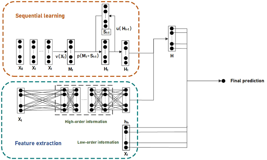
Figure 1. The overview of the proposed forecasting model.

2.1. Sequential Learning Component

The recurrent neural network (RNN) based models are more suitable for time series fitting tasks with time dependencies than the normal artificial neural network (ANN). Due to the weather and seasonal features of the tourism data, (a) we design an RNN model that has the ability for sequential learning to explore the short-term dependencies in tourism time series. The main function of RNN based models is to interact the current information with the historical state. In our network, the state of the hidden layers is updated as follows:

$\begin{array}{c}{S}_{t-1}=u(H_{t-1})\\ M_t=v(X_t)\\ H_t=p(M_t+S_{t-1})& (1)\end{array}$

where X_t denotes the features at time t, H_t denotes the state of the hidden layer at time t, u(·) transform the state of hidden layer at t − 1, v(·) extracts the information within X_t and p(·) joints the relevant contextual at time t − 1 and t. Thus, the current state of the hidden layer is updated and transferred. In our network, the functions u(·), v(·), and p(·) are defined as follows:

$\begin{array}{c}u\left(H_{t-1}\right)=relu\left(V_2^{T}relu\left(V_1^T{H}_{t-1}+b_1\right)+b_2\right)\\ v\left(X_t\right)=\sigma \left(U_2^T\left(relu\left(U_1^T{X}_t+b_3\right)+b_4\right)\right)\\ p\left(M_t+S_{t-1}\right)=\sigma \left(M_t+S_{t-1}\right)& (2)\end{array}$

where U, W, and b are parameters that are trained at each step t. The symbol relu(·), σ(·) are denoted as relu and sigmoid function, respectively.

2.1.1. Feature Extracting Component

Different correlations of features in the tourism data contains different information. In order to better extract the informative correlations in features, we design two modules that can be executed in parallel in feature extracting component, which are utilized to extract high-order and low-order information in tourism data.

For extracting the low-order information, we design a single-layer fully connected neural network to explore the linear relation in tourism data. It transforms features by combining features in different dimensions linearly. The module is defined as:

$\begin{array}{ll}{r}_l=w_l^{\text{T}}{X}_t+b_l,& (3)\end{array}$

where X_t denotes the features of the target time t, r_l is the linear combination of features. $w_l\in {ℝ}^n$ is the parameters serve as the coefficients for linear weighting.

We devise another model for extracting high-order correlations in features. This module leverages the powerful non-linear expressing capability of multi-layer perceptrons to extract complex but valuable correlations in features. This module can be formally defined as follows:

$\begin{array}{c}{h}_1={\gamma }_0\left(W_0^{\text{T}}{X}_t+b_0\right)\\ h_2={\gamma }_1\left(W_1^{\text{T}}{h}_1+b_1\right)\\ \cdots \cdots \\ h_{n+1}={\gamma }_n\left(W_n^{\text{T}}{h}_n+b_n\right)\\ h_h=\sigma \left(W_{n+1}^{\text{T}}{h}_{n+1}+b_{n+1}\right)& (4)\end{array}$

where n denotes n-th hidden layer, W_n, b_n, γ_n(·), and h_n+1 are the weight matrix, bias, activation function and output of (n + 1)-th hidden layer, respectively. W_n+1, b_n+1, σ(·), and h_h are the weight matrix, bias, activation function, and output of output layer, respectively. This module takes the features X_t as inputs, and output the h_h as the high-order combination of features. Finally, the output of the forecasting model is combined as follows:

$\begin{array}{c}H=H_t+h_h\\ r_f=W_u^{T}f\left(W_v^{T}H+b_v\right)+b_u\\ {Ŷ}_t=r_l+r_f& (5)\end{array}$

Here, the high-order information is combined with the output of sequential learning part. Then the result is in turn combined with the output of low-order information to form the prediction of the future value at time t.

2.2. Ensemble Method

The above design rely on single model for forecasting. By combining multiple sub-models, ensemble learning often results in significantly superior generalization performance over a single model. In this section we propose an ensemble learning scheme that can boost the accuracy of the forecasting model. Our design based on the observation that tourism data happen in same time can be classified into different category (e.g., year, region, etc.), which we defined as band. Sequence data happens in different band but same time can be combined to improve the robustness of the model prediction. The proposed approach can be divided into the following steps:

(1) Features division

The method extract features {X₁, X₂, ⋯ , x_T} from times series {x₁, x₂, ⋯ , x_T}, and then the features are divided into several bands as

$\begin{array}{ll}{\text{X}}_t=\left\{X_t^1,X_t^2,\cdots ,X_t^m\right\}(t=1,2,\cdots ,T)& (6)\end{array}$

where each features at time point t are divided into m sub-features.

(2) Features reconstruction.

To obtain more representative features for the models, the original features have been reconstructed in this step as following,

$\begin{array}{ll}D=\left\{X_t^{1\prime },X_t^{2\prime },\cdots ,X_t^{N\prime }\right\}& (7)\end{array}$

where D denotes the new features set, and each features at time point t are reconstruct into N sub-features.

(3) Sub-models results on the new feature data

Each model has been trained using the reconstructed features to obtaining the following results,

$\begin{array}{ll}\varphi (D)=\left\{{\varphi }_1(X_t^{1\prime }),{\varphi }_2(X_t^{2\prime }),\cdots ,{\varphi }_N(X_t^{N\prime })\right\}& (8)\end{array}$

where ϕ_i, i = 1, 2, ⋯ , N are the sub-models adopted in the proposed approach.

(4) Models ensemble

After the above three steps, we can obtain the sub-models for each sub-feature, after then, the operator of Com has been adopted to obtain the ensemble model. The overview of the ensemble method is presented as Figure 2.

$\begin{array}{ll}{\Phi }_{c,t}=Com\left\{{\varphi }_1(X_t^{1\prime }),{\varphi }_2(X_t^{2\prime }),\cdots ,{\varphi }_N(X_t^{N\prime })\right\}& (9)\end{array}$

where ϕ_c,t denotes the final results of at time point t. ϕ presents a particular transformation method, such as stacking, hadmard product or linear combination. Based on the combination, we can form multiple sub-models to explore the relations in different bands. The process of the ensemble method is shown in Algorithm 1:

FIGURE 2

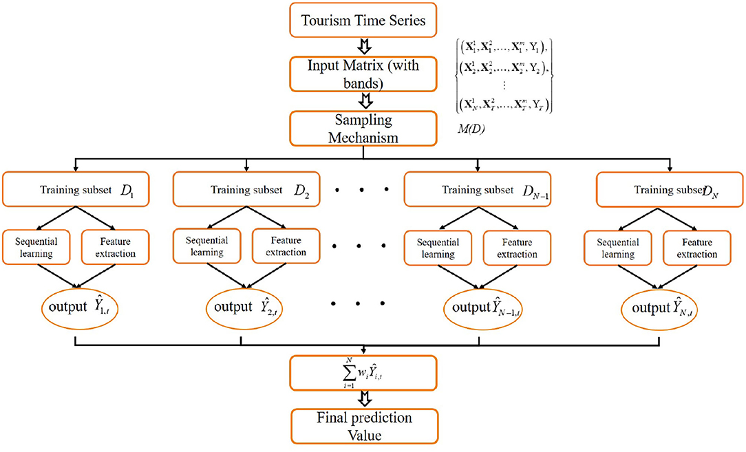
Figure 2. The overview of the proposed ensemble scheme.

ALGORITHM 1

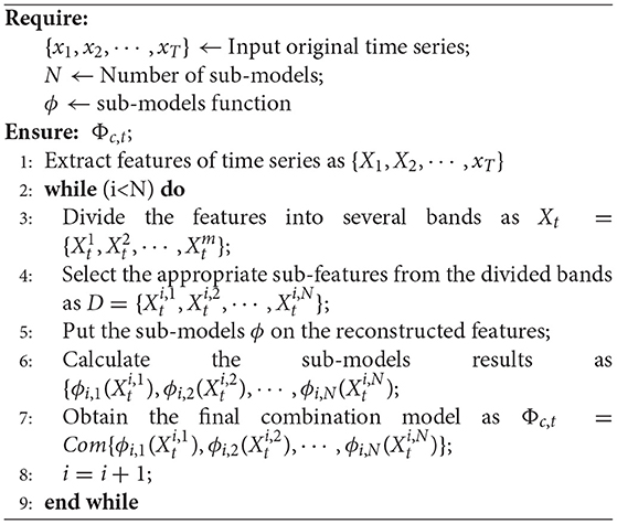
Algorithm 1 The proposed ensemble algorithm.

3. Experimental Evaluation

3.1. Dataset Description

In this article, the tourism demand time series from Cheng du Research Base of Giant Panda Breeding¹ (TDPB) is used in our experiment, as shown in Figure 3. Cheng du Research Base of Giant Panda Breeding, located at 1375# Panda Road, Northern Suburb, Chenghua District, Chengdu City, Sichuan Province, P.R.China, is 10 km away from the city center and over 30 km from Chengdu Shuangliu International Airport. Proclaimed the “ecological demonstration project for the ex-situ conservation of giant pandas.” The Base, covering an area of 1,000 mu (66.67 hectares), serves as the world's torchbearer for the ex-situ conservation of giant pandas, scientific research and breeding, public education, and educational tourism. The Base wears its title very well as the sanctuary for giant pandas, red pandas, and other endangered wild animals exclusive to China. TDPB covers the number of visitors to the panda base from 2017 to 2021, with a total of 1,826 pieces of data. The largest number of visitors was on October 4,2018, with 102,305 visitors. The corresponding statistics are shown in the following Table 1.

FIGURE 3

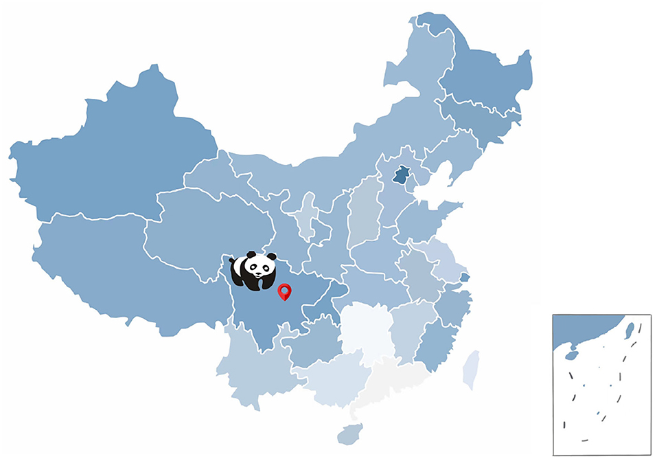
Figure 3. The Chengdu research base of giant panda breeding.

TABLE 1

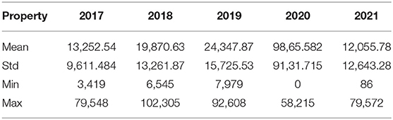
Table 1. The datasets used in our experiments.

3.2. Evaluation Indicator

To evaluate the effectiveness of our scheme, we use the Root Mean Square Error (RMSE), mean absolute error (MAE), and Mean Absolute Percentage Error (MAPE) metrics to measure the accuracy of the estimates. These metrics are defined as:

$\begin{array}{ll}\text{MAPE}=\frac{1}{N}{\displaystyle \sum _{t=1}^N}\left|\frac{Y_t-{Ŷ}_t}{Y_t}\right|\times 100\%,& (10)\end{array}$

$\begin{array}{ll}\text{RMSE}=\sqrt{\frac{1}{N}{\displaystyle \sum _{t=1}^N}{\left(Y_t-{Ŷ}_t\right)}^2},& (11)\end{array}$

$\begin{array}{ll}\text{MAE}=\frac{{\displaystyle {\sum }_{t=1}^N}|Y_t-{Ŷ}_t|}{N},& (12)\end{array}$

where Y_t and Ŷ_t are the actual demand and predicted demand of future value at time t, respectively, and N denotes the maximum time being predicted in the test set. Clearly, smaller value of the three metrics indicates better forecasting results.

3.3. Other SCHEMES and Parameter Selection

To evaluate the performance of our scheme, we compare it with some state-of-the-art tourism demand forecasting techniques, listed as follows.

• Decision Tree (DT) (Song and Ying, 2015): DT falls under the category of supervised learning. It uses the tree representation to solve the problem in which each leaf node corresponds to a class label and attributes are represented on the internal node of the tree.

• Random Forest (RF) (Kane et al., 2014): RF is a supervised machine learning algorithm that is constructed from multiple decision tree. And RF is a classic ensemble learning algorithm for regression and classification.

• Extra Trees (ET) (Hammed et al., 2021): ET also known as Extremely Randomized Trees. Similar to RF, ET builds multiple trees and splits nodes using random subsets of features. Different from RF, ET uses the whole learning sample and splits nodes by choosing cut-points fully at random.

• Gradient Boosting (GB) (Gong et al., 2020): GB is an supervised machine learning algorithm used for classification and regression problems. It is an ensemble technique which uses multiple weak learners to produce a strong model for regression and classification. GB relies on the intuition that the best possible next model, when combined with the previous models, minimizes the overall prediction errors. The key idea is to set the target outcomes from the previous models to the next model in order to minimize the errors.

• Light Gradient Boosting Machine (LGB) (Fan et al., 2019): LGB is a gradient boosting framework based on decision trees to increase the efficiency of the model. LGB has been widely used in time series problems. And LGB is one of the most popular time series models.

• Extreme Gradient Boosting (XGBoost) (Chen et al., 2015): XGBoost is a decision trees based ensemble method which makes use of gradient boosting. It is one of the most powerful algorithms for regression and classification with high speed and performance.

In this dataset, the main factors we consider include holidays, weather, and the number of visitors a few days before the forecasted date. In our experiment, each model uses the same feature input to ensure that the model does not differ in performance due to inconsistent input information. In the proposed model, we separately verified the performance of the RNN module and DNN module with different numbers of neurons in the hidden layer (32, 64, 128, 256, 512). The parameters are initialized using the popular Xavier's approach (Glorot and Bengio, 2010), and the optimizer is stochastic gradient descent algorithm (Bottou, 2012).

3.4. Experimental Results and Analysis

The forecasting results on test set are reported in Table 2 and Figure 4. Table 2 reports the test results of our experiments on RMSE, MAE, MAPE. It can be seen from Table 2 that our scheme performs better than other algorithms in RMSE, MAE, and MAPE. Compared with the Decision Tree, ensemble models achieve better performance since they can effectively mine more valuable information. In RMSE, our scheme achieves the best performance with 5673.635, and Random Forest achieves the second best performance with 7790.284, and other models are over 7,800. Similar to RMSE, the MAE value of the proposed scheme outperforms other models, and our scheme achieves at least 1,119 improvement. In terms of MAPE metric, our scheme achieves the lowest value of 26.05%, while the corresponding values of other ensemble models are about 44%. The main reason for this accuracy improvement is that our scheme incorporates historical information and some environmental factors, and extracts high-order features and low-order features from the original data through the feature extracting component and sequential learning component.

TABLE 2

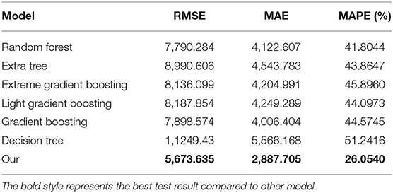
Table 2. The values of RMSE, MAE, and MAPE results for different methods.

FIGURE 4

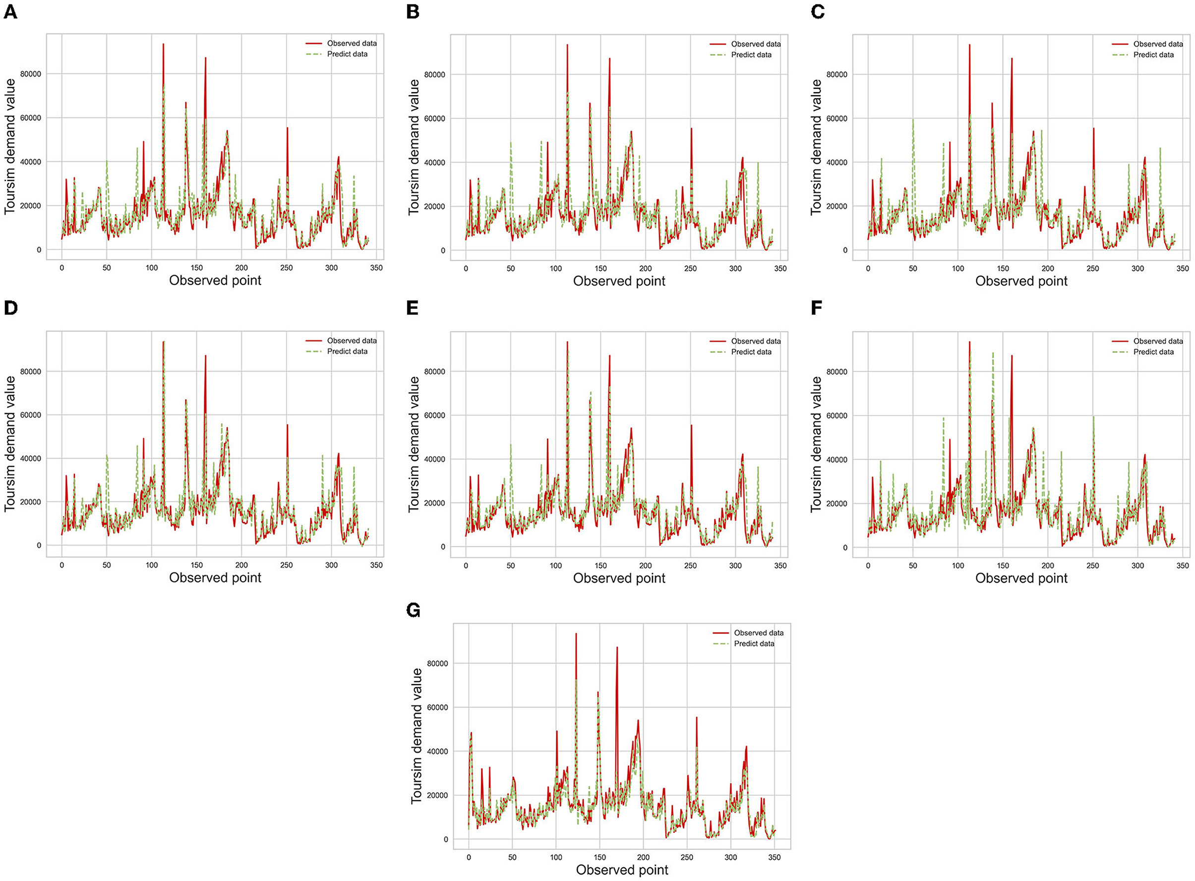
Figure 4. The overview of the forecasting results in different model. (A) Forecasting results of RF, (B) forecasting results of ET, (C) forecasting results of LGB, (D) forecasting results of XGBoost, (E) forecasting results of GB, (F) forecasting results of DT, (G) forecasting results of Ours.

Figure 4 draws the observed tourism demand and the forecasting results of different algorithms. Compared with other algorithms, the results of our schemes fits the actual results with the smallest gap. Compared with Figure 4G, the forecasting results of these algorithms have low accuracy at specific times. Around the 50-th forecasting date, the Figure 4G shows there is a significant gab between predicted demands and the actual demands from Figures 4A–F, and our scheme avoids this phenomenon as shown in Figure 4G. The accuracy improvement can be attributed to the effectiveness of our models for extracting useful information through the recurrent neural network, and the tree-based ensemble models only consider the information of the forecasting date.

To make the conclusions are more believable and robust. We have compared the forecasting results before the outbreak of COVID-19 and after the outbreak of COVID-19, as shown in Tables 3, 4. Table 3 reports the test results for each month of 2019. It can be seen that in most of cases, the proposed approach can obtain the desire forecasting performance. The results indicate that the proposed model achieves the best performance in January, February, April, June, and December in terms of MAE values. Furthermore, for MAPE values, the proposed model performs better than other algorithms in January, February, April, November, and December, as well as outperforms other algorithms on RMSE in January, February, April, June, and November. Our method holds a good performance in January in terms of all metrics, the number of tourists in January is unstable, because the Spring Festival of 2019 is not in January but the winter holiday is beginning in January. What's more, the proposed model also performs well in November and December, there is no official holiday in these 2 months, therefore, the proposed model can both fit the data tendency of peaks and valleys. In general, the mean values of the proposed model in this study performs better than other algorithms. The mean MAE value of our proposed model is 4175.32, which is lower than other compared models and can improve about 700. Similarly, the proposed model can also achieve the desire results in terms of the mean value of MAPE, it owns MAPE value of 16.08% and improves the worst model (DT) about 20%. Otherwise, the same tendency also existed in the metric of RMSE. The averaged MAPE values of our method is 19.96, 9.37, 9.26, 13.85, 13.67, and 7.77%, which are lower than DT, ET, GB, LGB, RF, and XGBoost, respectively. Therefore, the proposed approach in this study achieves the highest accuracy in most cases, which validates the superiority in extracting nonlinear features and useful information in TDPB through sequential learning and feature extracting components.

TABLE 3

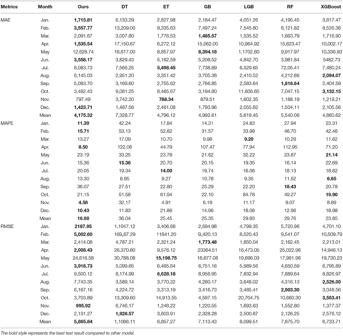
Table 3. Forecasting results in 2019.

TABLE 4

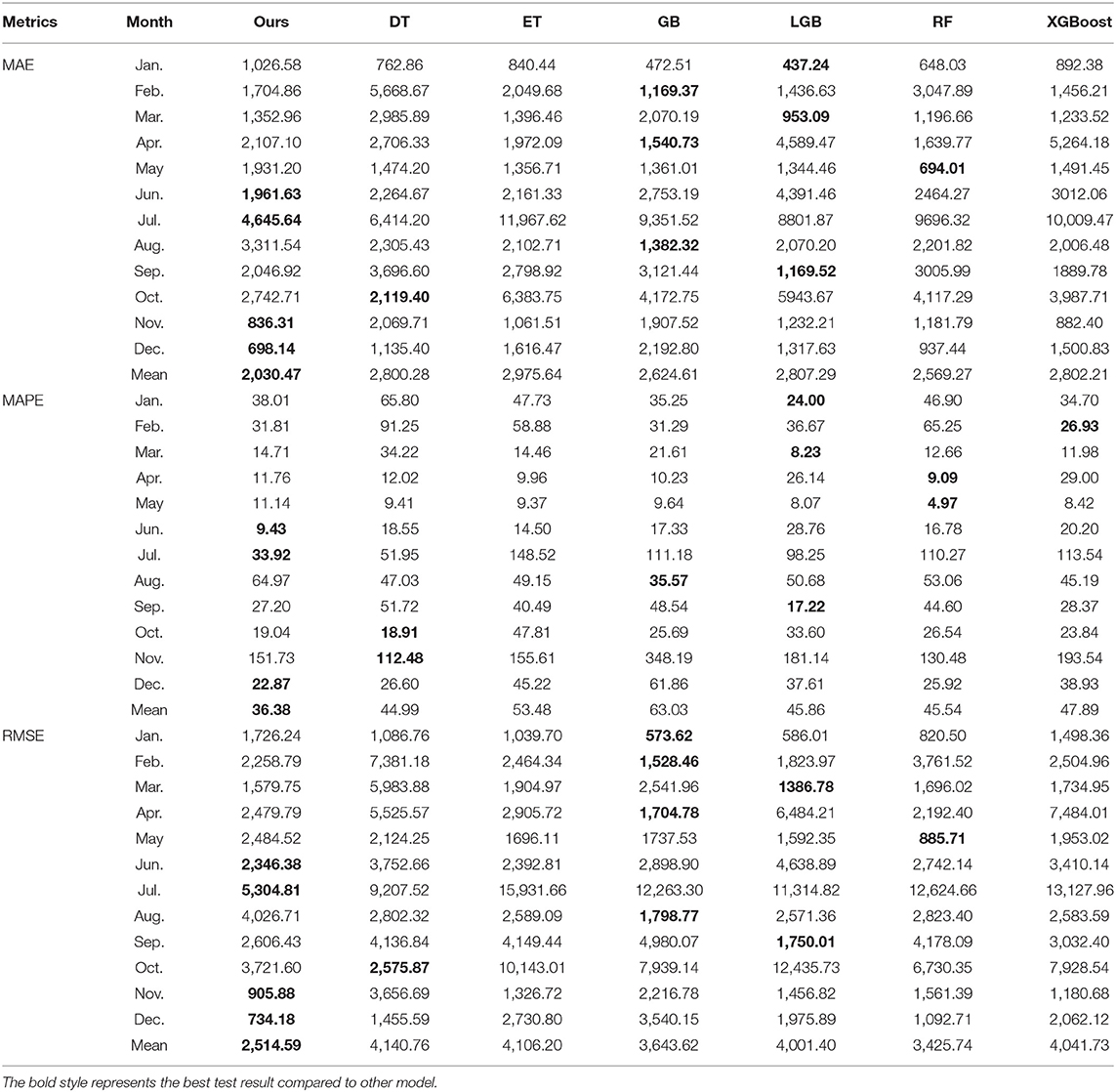
Table 4. Forecasting results in 2021.

Table 4 lists the forecasting results for each month of 2021, the results are worse than the results of 2019, which is mainly caused by the outbreak of COVID-19. Where the COVID-19 occurs in the end 2019, the local government introduce policies to restrict tourism, therefore, the data set of 2020 shows a large fluctuation comparing to the previous years, in this way, the use of data set of 2020 has a negative effect on the model building. The results indicate that our proposed model has a good performance in June, July, November, and December both in MAE, MAPE, and RMSE values. However, comparing with other models, the mean results of our proposed model are superior. After 2020, at the beginning of each year, the repeat outbreak of COVID-19 makes the number of tourists is uncertainty. Therefore, the proposed model is failed to forecast the results of January, February and so on, but it is adapted by itself after the May. It can be seen from Table 4 that the proposed scheme obtains the best MAPE in 2021 with 36.38%, and achieves 8.61, 17.09, 26.65, 9.48, 9.16, and 11.50% improvement over DT, ET, GB, LGB, RF, and XGBoost, respectively. Other two metrics of MAE and RMSE also support the same conclusions. Similar to 2019, the proposed scheme outperforms other models.

Comparing Tables 3, 4, it can be found that the MAPE value of each model in 2021 is obviously higher than in 2019. Different from 2019, 2021 is the time after the COVID-19 outbreak. As we all known, China government imposes some travel restrictions during COVID-19. Although some contingencies are not considered in our scheme, our scheme still achieves the best accuracy performance, which indicates that our scheme has stronger robustness. Overall, the above experimental results demonstrate that the proposed scheme universally and consistently provide the best accuracy in all test set. This demonstrates the robustness of our method against the unexpected factors including travel restrictions. This also validates the effectiveness of sequential learning component for capturing the corresponding the difference in time.

4. Conclusion

Chengdu Research Base of Giant Panda Breeding is the top attractions both at home and abroad. Effective tourism demand forecasting of Chengdu Research Base of Giant Panda Breeding can help managements balance the hotel, traffic, and other public resources. This article proposes an ensemble learning based model for tourism demand forecasting considering environmental factors. The proposed scheme can both explore the sequential relation in tourism time series and extract valuable correlation in features of the estimate time through sequential learning component and feature extracting component. The ensemble method is proposed to fuse multiple forecasting results from sub-models with reconstructed forecasting input. Experimental results on the tourism demand time series from Chengdu Research Base of Giant Panda Breeding demonstrate that the proposed ensemble learning based model not only can achieve higher forecasting accuracy, but also has stronger robustness. Thus, the proposed model holds potential to be widely applied in tourism industry.

Data Availability Statement

The raw data supporting the conclusions of this article will be made available by the authors, without undue reservation.

Author Contributions

JH: writing, conceptualization, and methodology. DL: modeling and writing and editing. YG: data collection and processing. DZ: data processing and model programming. All authors contributed to the article and approved the submitted version.

Funding

This work was supported by the Central Guidance on Local Science and Technology Development Fund of Sichuan Province (2021ZYD0156).

Conflict of Interest

DZ was employed by Chengdu Zhongke Daqi Software Co., Ltd.

The remaining authors declare that the research was conducted in the absence of any commercial or financial relationships that could be construed as a potential conflict of interest.

Publisher's Note

All claims expressed in this article are solely those of the authors and do not necessarily represent those of their affiliated organizations, or those of the publisher, the editors and the reviewers. Any product that may be evaluated in this article, or claim that may be made by its manufacturer, is not guaranteed or endorsed by the publisher.

Footnote

1. ^http://www.panda.org.cn/english/

References

Bottou, L. (2012). “Stochastic gradient descent tricks,” in Neural Networks: Tricks of the Trade. Lecture Notes in Computer Science, Vol. 7700, eds G. Montavon, G. B. Orr, and K. R. Müller (Berlin; Heidelberg: Springer). doi: 10.1007/978-3-642-35289-8_25

CrossRef Full Text | Google Scholar

Chen, T., He, T., Benesty, M., Khotilovich, V., Tang, Y., Cho, H., et al. (2015). Xgboost: Extreme Gradient Boosting. R Package Version 0.4-2, 1–4. Available online at: https://cran.r-project.org/web/packages/xgboost/ (accessed April 26, 2022).

Google Scholar

Claveria, O., Monte, E., and Torra, S. (2015). Common trends in international tourism demand: are they useful to improve tourism predictions? Tour. Manage. Perspect. 16, 116–122. doi: 10.1016/j.tmp.2015.07.013

CrossRef Full Text | Google Scholar

Fan, J., Ma, X., Wu, L., Zhang, F., Yu, X., and Zeng, W. (2019). Light gradient boosting machine: an efficient soft computing model for estimating daily reference evapotranspiration with local and external meteorological data. Agric. Water Manage. 225, 105758. doi: 10.1016/j.agwat.2019.105758

CrossRef Full Text | Google Scholar

Faruk, D. Ö. (2010). A hybrid neural network and ARIMA model for water quality time series prediction. Eng. Appl. Artif. Intell. 23, 586–594. doi: 10.1016/j.engappai.2009.09.015

CrossRef Full Text | Google Scholar

Glorot, X., and Bengio, Y. (2010). “Understanding the difficulty of training deep feedforward neural networks,” in Appearing in Proceedings of the 13th International Conference on Artificial Intelligence and Statistics (AISTATS) 2010, (Sardinia), 249–256.

Google Scholar

Gong, M., Bai, Y., Qin, J., Wang, J., Yang, P., and Wang, S. (2020). Gradient boosting machine for predicting return temperature of district heating system: a case study for residential buildings in Tianjin. J. Build. Eng. 27, 100950. doi: 10.1016/j.jobe.2019.100950

CrossRef Full Text | Google Scholar

Hammed, M. M., AlOmar, M. K., Khaleel, F., and Al-Ansari, N. (2021). An extra tree regression model for discharge coefficient prediction: novel, practical applications in the hydraulic sector and future research directions. Math. Probl. Eng. 2021, 7001710. doi: 10.1155/2021/7001710

CrossRef Full Text | Google Scholar

Hao, Y., Niu, X., and Wang, J. (2021). Impacts of haze pollution on china's tourism industry: a system of economic loss analysis. J. Environ. Manage. 295, 113051. doi: 10.1016/j.jenvman.2021.113051

PubMed Abstract | CrossRef Full Text | Google Scholar

Ji, L., Zou, Y., He, K., and Zhu, B. (2019). Carbon futures price forecasting based with ARIMA-CNN-LSTM model. Proc. Comput. Sci. 162, 33–38. doi: 10.1016/j.procs.2019.11.254

PubMed Abstract | CrossRef Full Text | Google Scholar

Kane, M. J., Price, N., Scotch, M., and Rabinowitz, P. (2014). Comparison of ARIMA and random forest time series models for prediction of avian influenza h5n1 outbreaks. BMC Bioinformatics 15, 276. doi: 10.1186/1471-2105-15-276

PubMed Abstract | CrossRef Full Text | Google Scholar

Khademi, Z., Ebrahimi, F., and Kordy, H. M. (2022). A transfer learning-based CNN and LSTM hybrid deep learning model to classify motor imagery EEG signals. Comput. Biol. Med. 2022, 105288. doi: 10.1016/j.compbiomed.2022.105288

PubMed Abstract | CrossRef Full Text | Google Scholar

LeCun, Y., and Bengio, Y. (1995). “Convolutional networks for images, speech, and time series,” in The Handbook of Brain Theory and Neural Networks, ed M. Arbib (Cambirdge, MA: MIT Press), 255–258.

Li, Y., and Cao, H. (2018). Prediction for tourism flow based on lstm neural network. Proc. Comput. Sci. 129, 277–283. doi: 10.1016/j.procs.2018.03.076

CrossRef Full Text | Google Scholar

Liu, X., Peng, H., Bai, Y., Zhu, Y., and Liao, L. (2014). Tourism flows prediction based on an improved grey GM (1, 1) model. Proc. Soc. Behav. Sci. 138, 767–775. doi: 10.1016/j.sbspro.2014.07.256

CrossRef Full Text | Google Scholar

Ozkok, F. O., and Celik, M. (2022). A hybrid CNN-LSTM model for high resolution melting curve classification. Biomed. Signal Process. Control 71, 103168. doi: 10.1016/j.bspc.2021.103168

CrossRef Full Text | Google Scholar

Qian, L., Zhao, J., and Ma, Y. (2022). Option pricing based on GA-BP neural network. Proc. Comput. Sci. 199, 1340–1354. doi: 10.1016/j.procs.2022.01.170

CrossRef Full Text | Google Scholar

Shin, H.-C., Roth, H. R., Gao, M., Lu, L., Xu, Z., Nogues, I., et al. (2016). Deep convolutional neural networks for computer-aided detection: CNN architectures, dataset characteristics and transfer learning. IEEE Trans. Med. Imaging 35, 1285–1298. doi: 10.1109/TMI.2016.2528162

PubMed Abstract | CrossRef Full Text | Google Scholar

Singh, K. R., Neethu, K., Madhurekaa, K., Harita, A., and Mohan, P. (2021). Parallel SVM model for forest fire prediction. Soft Comput. Lett. 31, 00014. doi: 10.1016/j.socl.2021.100014

CrossRef Full Text | Google Scholar

Song, Y.-Y., and Ying, L. (2015). Decision tree methods: applications for classification and prediction. Shanghai Arch. Psychiatry 27, 130. doi: 10.11919/j.issn.1002-0829.215044

PubMed Abstract | CrossRef Full Text | Google Scholar

Wang, H.-J., Jin, T., Wang, H., and Su, D. (2022). Application of ieho-bp neural network in forecasting building cooling and heating load. Energy Rep. 8, 455–465. doi: 10.1016/j.egyr.2022.01.216

CrossRef Full Text | Google Scholar

Wang, X. (2022). Research on the prediction of per capita coal consumption based on the ARIMA-BP combined model. Energy Rep. 8, 285–294. doi: 10.1016/j.egyr.2022.01.131

CrossRef Full Text | Google Scholar

Yu, H. (2021). Development of tourism resources based on fpga microprocessor and convolutional neural network. Microprocess. Microsyst. 82, 103795. doi: 10.1016/j.micpro.2020.103795

CrossRef Full Text | Google Scholar