A Fly in the Ointment: How to Predict Environmentally Driven Phenology of an Organism That Partially Regulates Its Microclimate

Phenological models representing physiological and behavioral processes of organisms are used to study, predict, and optimize management of ecological subsystems. One application of phenological models is the prediction of temporal intervals associated with the measurable physiological development of arthropods, for the purpose of estimating future time points of interest such as the emergence of adults, or estimating past time points such as the arrival of ovipositing females to new resources. The second of these applications is of particular use in the conduct of forensic investigations, where the time of a suspicious death must be estimated on the basis of evidence, including arthropods with measurable size/age, found at the death scene. Because of the longstanding practice of using necrophagous insects to estimate time of death, standardized data and methods exist. We noticed a pattern in forensic entomological validation studies: bias in the values of a model parameter is associated with improved model fit to data, for a reason that is inconsistent with how the models used in this practice are interpreted. We hypothesized that biased estimates for a threshold parameter, representing the lowest temperature at which insect development is expected to occur, result in models’ accounting for behavioral and physiological thermoregulation but in a way that results in low predictive reliability and narrowed applicability of models involving these biased parameter estimates. We explored a more realistic way to incorporate thermoregulation into insect phenology models with forensic entomology as use context, and found that doing so results in improved and more robust predictive models of insect phenology.

Introduction

The prediction of phenology or physiological development as a function of ecological and environmental factors facilitates study and management of many types of ecosystems, with a mature application being the modeling of insect development to estimate time points of interest (Catts, 1992; Catts and Goff, 1992; Amendt et al., 2007; Byrd and Tomberlin, 2019). Estimating insect developmental rates and intervals is useful for the management of insects (pests or beneficial species alike), and can be employed in optimizing intervention times or allocation of monitoring resources (e.g., Chappell et al., 2020; Crimmins et al., 2020). The ability to accurately estimate temporal intervals on a case-by-case basis is especially valuable in the conduct of forensic investigations where the interval of interest is the time between a death and the discovery of human remains, and for this reason the application of phenology models has been studied regularly by forensic entomologists (Catts and Haskell, 1990; Catts, 1992; Catts and Goff, 1992; Grassberger and Reiter, 2001, 2002a,b; Amendt et al., 2007; Michaud and Moreau, 2011; Tarone and Sanford, 2017; Byrd and Tomberlin, 2019; Matuszewski, 2021). Through understanding the processes of insect development, forensic investigators are able to estimate temporal information related to a death, often considered to reflect the postmortem interval (PMI) or minimum postmortem interval (mPMI) (Tarone and Sanford, 2017). Many such applications of insect phenology models are common in ecology and agriculture, and continued improvement of the models requires ongoing research into phenology to increase model realism.

Models of insect phenology generally predict physiological age as a function of abiotic inputs: the interaction between an individual organism and its environment (especially the temperature of its environment) determines the rate of physiological development. Many applications of phenology model output are especially useful in cases of unusual or locally unprecedented abiotic conditions (e.g., Chappell et al., 2013), because these are situations in which inductive assumptions based on prior occurrences are likely to be invalid. For example, in conditions of extreme heat or cold, insects that develop as a function of heat may be present or active very early or late relative to their average phenology, with wide-ranging potential impacts to ecosystems both natural and managed (Kemp et al., 1986; Tobin et al., 2008; Singer and Parmesan, 2010). For accurate extrapolative predictions to be generated by a phenology model given unusual or unprecedented environmental conditions, the model must sufficiently capture the mechanisms relevant to organisms’ responses to environmental inputs. For example, climate change is expected to result in environmental conditions that are locally unprecedented, such that unprecedented phenological outcomes may be expected (Singer and Parmesan, 2010). For phenology models to continue providing useful output for ecosystems experiencing climate change, the models must be able to represent phenology in conditions that are potentially warmer or more variable than has been observed in situ to date.

In the spirit of Stephen Jay Gould’s baseball analogies which relate processes to statistics (and which are familiar to ecologists and evolutionary biologists) (e.g., Gould, 1992), the difference between description and prediction can be illustrated for phenology. It is possible to statistically predict the location on a field to which a specific batter will most likely hit a ball without having thorough mechanistic understanding of the processes involved. Concerning applications, shifting the fielding team’s position according to such a prediction will on average result in the most effective defense. However, on a day with strong winds, a model that does not account for the mechanistic relationship between wind and baseball trajectory will be inaccurate in predicting where the ball will go on that particular day. The particular challenge addressed here (and described in more detail below) is also interesting in that it seems to represent a situation where, in this analogy, the ball appears to want to land in a particular spot on the field, regardless of where it is hit. The details of a particular day on which baseball is played are analogous to the details of a particular forensic case, which may or may not conform to the expectations of a typical case. Thus, while models based on analysis of large numbers of scenarios are useful for capturing averages, a lack of mechanistic understanding can harm the application of scientific knowledge to a particular case – something that is desirable to avoid as much as is feasible in any forensic science application because of the consequences of individual predictions.

The insect phenology and development models used by forensic entomologists are standardized to a degree because of the nature of their use. In the United States of America, output from these models becomes part of scientific testimony which is subject to criteria for admissibility known as the “Daubert standard,” in reference to the United States Supreme Court case Daubert v. Merrell Dow Pharmaceuticals, Inc., in which the criteria were first articulated. Two of these criteria are that a given scientific technique must be accepted by the relevant scientific community, and that the technique must have standard operating procedures (Faigman, 2002; Amendt et al., 2007; Gaudry and Dourel, 2013; Sanford et al., 2019; Gelderman et al., 2021, also see OSAC, 2021). As a result, the insect phenology models used by forensic scientists are among the more standardized ecological models, which in turn results in the generation of intercomparable validation data due to standardized application. Additionally, studies aimed at validating the models have been conducted by forensic scientists, to purposefully investigate the appropriateness of their application across geographic space, in environmental or other conditions of interest, and to ensure that the models continue to serve the purposes for which they are used. Validation effort has been directed to several aspects of models used in forensic entomology: representativeness of microenvironmental temperatures by available ambient temperature data (Archer, 2004; Dourel et al., 2010; Johnson et al., 2014; Dabbs, 2015), accuracy of estimates for temperature “thresholds” below which physiological development ceases (Day and Rowe, 2002; Tarone et al., 2011; Cervantès et al., 2017), and empirical fit of model forms to relevant phenology data (Tarone and Foran, 2008; Baqué and Amendt, 2013). Development rate functions are typically fit to data generated by raising insects at constant temperatures, but temperature fluctuation has been studied as an effect on development since the modeling work of Kaufmann (1932) described the potential for rate summation across varying temperature to impart bias to development rate estimates, now called the “Kaufmann effect.” Proposed explanations for the effect have included the consequences of mathematical order of operations, for example a sum of a function-transformed variable, versus the functional transformation of a sum, the difference of which being proved in the theorem now known as Jensen’s Inequality (Jensen, 1906). Attempts to develop models that accurately predict instantaneous development rate under conditions of temperature fluctuation have shown that curvilinear or non-linear functions better describe development rate variation than do rectilinear ones, and that interpreting temperatures relative to an optimum can enhance predictive performance (Worner, 1992; Ikemoto, 2005; Ikemoto and Egami, 2013). Theoretical treatment of fundamental assumptions and mechanisms represented by phenology models in general is an enduring ecology research topic of interest (Stinner et al., 1974; Sharpe and DeMichele, 1977; Wagner et al., 1984; Post, 2019).

Validation studies that involve deployment of a model in its intended use context are an indispensable component of modeling research and application. Such studies may forfeit some ability to isolate causes in the way that laboratory studies can when focused on individual model parameters, but in-field validation is the only setting in which all assumptions and all aspects of a model can be confronted by realistic data. Forensic entomological validation studies that involve field data have been used for purposes such as assessing applicability or generality of models across geography or scenarios, recovering parameter estimates from data that are distributed across greater variability in conditions, or simply for quantifying error that should be expected as a result of using models in practically relevant scenarios (Tarone and Foran, 2008; VanLaerhoven, 2008; Matuszewski, 2011; Flores, 2013; Núñez–Vázquez et al., 2013; Harnden and Tomberlin, 2016; Matuszewski and Mądra-Bielewicz, 2016). While these aspects of model use are specific to a discipline, the conventions of that discipline are such that the example serves as a basis for addressing a general issue with empirical modeling, being the use of validation results to inform subsequent investigation, model development, and model utilization.

We recognized a pattern in the results of forensic entomology laboratory research and validation studies taken together: biased error in development threshold temperature (DTT) estimates. These thresholds, which can be species-specific (Higley and Haskell, 2001) or potentially vary within species (potential examples in Lamb, 1992; Gallagher et al., 2010; Tarone et al., 2011; Addeo et al., 2021) and represent a temperature above which development occurs as a function of temperature. At temperatures below DTT, environmental heat does not contribute to development. DTTs are used to adjust environmental temperature data so that summations of species-relevant heat units can be made. The conventional model used to predict insect development, the accumulated degree-day (ADD) model, outputs heat units as the product of temperature and time (typically degree-days), for temperatures above the DTT. For temperatures below the DTT, no development is accumulated per the model. Lower DTTs result in greater quantities of heat accumulation for two reasons: first, degree-days are always reported for a given DTT and any temperature’s degrees-above-DTT will be higher for a lower DTT; and second, lower temperatures are associated with development (non-zero degree-days) for lower DTT values. To estimate DTT, a function relating insect development rate to temperature can be used to extrapolate the temperature at which zero development should occur (Ikemoto and Takai, 2000; Ames and Turner, 2003). Laboratory control of environmental temperature simplifies the process of estimating DTT, and DTT is most commonly estimated under constant temperature.

Numerous studies have explored mathematical representations of development rates as functions of temperature (e.g., Sharpe and DeMichele, 1977; Schoolfield et al., 1981; many more reviewed in Wagner et al., 1984), with some of these obviating the need to include a DTT. However, logical and operational considerations limit the application of such models (Lamb et al., 1984), and inadequate performance increases over more parsimonious (and more readily conforming to the Daubert standard, in the case of forensic practice) models have prevented general adoption of perhaps more realistic but less generalizable models for insect phenology prediction. We commenced a modeling study motivated by the three findings described earlier: (1) the existence of models that are more realistic than the simplified linear ADD model, but which do not offer appreciable predictive performance increase (suggesting that the simplified ADD model accounts for more biological mechanisms than are explicit in the formulation); (2) DTT estimates including some that are lower than can be empirically corroborated in terms of physiology; and (3) researcher and practitioner use of different DTT depending on season or geography (Saunders and Hayward, 1998; VanLaerhoven, 2008). We asked why a known-underspecified model would perform as well or better than a more realistic one for insect phenology, and what the consequence of DTT estimation error may be for phenology prediction. Modeling revealed that biased DTT estimation can cause a linear ADD model to better fit a field-validation dataset, and as we will argue, one reason for this improvement is that a negatively biased DTT results in an increased correlation between heat accumulation and the passage of time. The reason for improved fit is not physiological per se, but rather because increasing the heat-time correlation allows the model to accommodate behavioral thermoregulation, the importance of which is reduced in controlled-temperature laboratory studies vs. the field where models are validated. For this and other reasons, temperature data has been aptly described as the “weak point” of forensic entomology (Charabidze and Hedouin, 2019), and it is similarly a weak point in related disciplines that seek to predict ectotherm physiology or phenology as functions of temperature, such as agricultural pest management or medical/veterinary vector ecology. In situations of changing climate and unprecedented variability, it is a modeling issue of general importance to have predictive models that fit well for valid reasons and require minimal calibration, and capture the processes through which organisms affect the microclimates that in turn determine development (Kaspari, 2019; Pincebourde and Casas, 2019).

Materials and Methods

Models

We begin with the general accumulated degree-day (ADD) model that is commonly used in the practice of medicolegal death investigations by practicing forensic entomologists (after Catts and Goff, 1992; Byrd and Tomberlin, 2019):

$$\forall T>DTT,Rat{e}_{Devel.}=\mathrm{\beta }\cdot \left(\mathrm{T}-\mathrm{DTT}\right)$$

$$\forall T\le DTT,Rat{e}_{Devel.}=0(1)$$

in which T is a variable describing momentary temperature recorded periodically at some interval, DTT is the development temperature threshold below which development is set to zero in the model, and β is a parameter relating change in temperature to change in development rate. Though there are both lower and upper temperatures beyond which development ceases, often in practice only a lower threshold as DTT is used in ADD calculation. Hence, in this study DTT represents only the lower developmental threshold. We call this the general model because the functional relationship it includes for temperature vs. development rate is strictly rectilinear, whereas less general models can involve curvilinear functional relationships, often based on empirically described growth curves (e.g., Byrd and Butler, 1996). The principal reason for our focus on this general model is its direct involvement in the field and other validation studies, wherein adjustment of DTT can be demonstrated to affect model fit.

A translation of the general model results in output in units of developmental time instead of a rate:

$$Development={\int }_{t_{Begin}}^{t_{End}}(\mathrm{\beta }\cdot (\mathrm{T}-\mathrm{DTT}))\mathit{d}t(2)$$

in which the temporal interval during which development occurs is arbitrarily defined or unknown, spanning the “begin” and “end” time points. If defined for the purpose of parameter estimation, this development interval can be the time between the oviposition of an egg and its hatching, or the duration of a larval instar, or a combination of life stages such as those between egg and adult. If unknown and the model is used to predict the interval given insect developmental ages and temperature data, the value of t_Begin or t_End is optimized for fit to data, often iteratively in practice. Also in practice, the integral is often approximated by summation, considering the periodicity of temperature measurements (e.g., hourly) and the conversion of output to desired time units (e.g., days).

Our approach was first to investigate the consequences on development interval estimation that result from changing the value of DTT. Because DTT is conventionally estimated by extrapolating from a fit of calculated development rates as a function of temperature, values of DTT are not typically empirically estimated at the time of estimating the value of β in Eq. 1. Thus, the ADD equations used by forensic entomologists are definitively non-linear in the parameters (β and DTT). The blow fly species Lucilia sericata and Cochliomyia macellaria are common in southern Texas and were commonly observed in our field sites, and we thus chose a DTT of 8°C because DTT for these species have been reported as 8°C for L. sericata (Reibe et al., 2010) or can be estimated from published results concerning C. macellaria as 8.5°C (data from Byrd and Butler, 1996) or 9.2°C (data from Boatright and Tomberlin, 2010). A DTT of 8°C is general with respect to varying blow fly species in our observation. To investigate the consequences of using negatively biased DTT, we explored multiple values iteratively.

We expected there to be a reason why increasing the correlation between heat accumulation and the passage of time would increase model’s predictive performance, and considered that endotherm/homeotherm development is highly predictable on the basis of time irrespective of environmental thermal variation, because of regulation through both physiological and behavioral processes. To investigate the use of more mechanistic interpretations of behavioral thermoregulation in phenology models for insects, we developed a way to use biased ambient temperatures to drive accumulated degree-day models of the forms shown above. We use ambient temperatures to estimate a derivative variable, T_reg:

$$T_{reg}=T_{amb}-C\left(T_{amb}-T_{pref}\right)\cdot \text{P}\left(T_{pref}|T_{amb},Scal{e}_{f(T_{amb})}\right)(3)$$

in which the subscripts reg, amb, and pref indicate three temperatures: reg (a predicted value) indicates the expected temperature of an insect that is behaviorally thermoregulating, amb (an independent variable) indicates the ambient temperature given at the location for which a phenology estimate is desired, and pref (a parameter) indicates a temperature that is “preferred” by the subject insect exposed to a range of temperatures. C is a constant used to represent the degree to which the subject organism is thermoconforming (Angilletta, 2009): a value of zero for C indicates a completely thermoconforming organism, and a value of 1 for C indicates that the organism is maximally able to maintain preferred temperature depending on what temperatures are available in the local environment, as a function of processes such as niche construction, aggregation, or physiological thermoregulation (Heaton et al., 2018; Pincebourde and Casas, 2019; Aubernon et al., 2022). We expect that ectothermic organisms whose body temperature is determined by environmental input, but who can choose microenvironments in which to dwell, are homeothermic to a degree determined by the configuration of their local environments. The availability of preferred temperature in the local environment is represented as the probability P(T_pref) of the value T_pref given a distribution of temperatures with location parameter T_amb and a scale parameter Scale_f(Tamb), calculated as the probability of T_pref in a normal distribution centered at T_amb, to describe variation in temperature.

Equation 3 predicts insect temperature (as T_reg) as function of two generalities: the distribution of temperatures in the local environment, and the insect’s behavioral and physiological processes of thermoregulation. Behavioral processes include movement to non-randomly experience temperature, and physiological processes in blow fly larvae include metabolic heat generation. While additional processes are likely to be relevant, we use these as literature-supported examples of explanations for why insect temperatures can be different from ambient temperatures (Turner and Howard, 1992; Slone and Gruner, 2007; Charabidze et al., 2011; Heaton et al., 2014; Gruner et al., 2017). We use the term “preferred” in recognition of the potential for there to be a difference between an optimal temperature for development (or other process related to phenology) and the temperature that organisms seek out in local environments (Martin and Huey, 2008; Aubernon et al., 2016).

Data Collection

We used digital thermography to record surface temperatures of remains at individual time points, for the purpose of studying temperature distributions and selecting a way to represent them with a scale parameter in Eq. 3 (Figure 1). A FLIR 650sc infrared camera was used to record thermal images. As decomposition progresses, insects become increasingly likely to be found at the surface of remains, such that thermographic images of remains were reasonable to use as a means of studying the shape environmental temperature distributions. Although we did not focus on human remains for this modeling study, we were contemporaneously collecting data from human remains at the Forensic Anthropology Research Facility (FARF) of the Forensic Anthropology Center at Texas State (FACTS) in San Marcos, Texas, and chose to use thermal images from human remains as a better basis than porcine remains for inferring T_pref. The reason for this decision was that human remains were more consistent in terms of size, age, and physical orientation in the field than were hogs used in our local study. We did not use human remains for regular observations of maggot masses due to logistical/geographic constraints. We used thermographic observation of human remains to generate a standard, the utility of which was thereafter tested in context of greater variation during our field study in College Station, Texas. Human cadavers that were thermographed were received by the FACTS under The Universal Anatomical Gift Act and were placed at the FARF by personnel there. Institutional Review Board (IRB) approval was not required for use of human cadavers because no personal or identifiable information was collected.

FIGURE 1

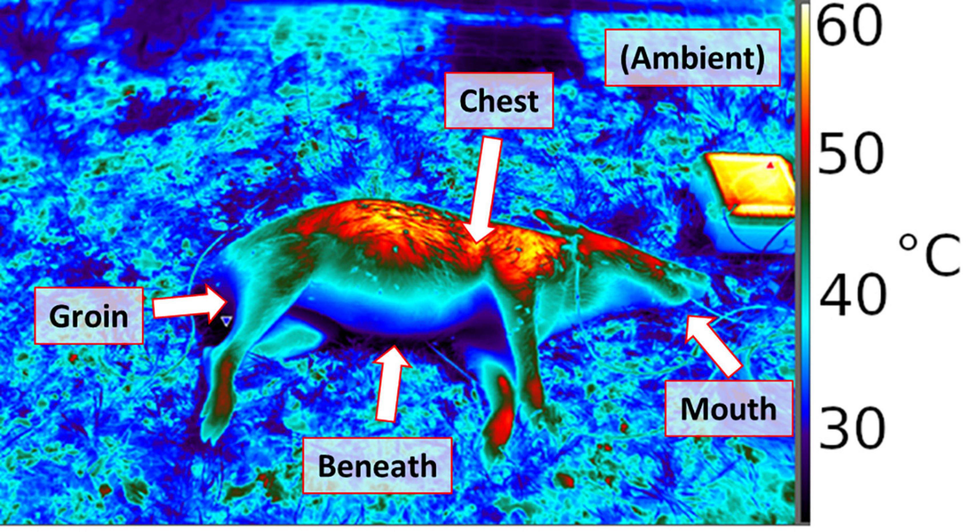
Figure 1. Thermograph of porcine remains placed in the field, using a FLIR 650sc infrared camera. Thermal probe positions are labeled.

A total of twelve hog carcasses donated by two landowners in south-central Texas, United States were obtained between 2018 and 2019. Each carcass was initially placed in a freezer for storage, and then partially thawed before being placed into the field at planned times, at the Texas A&M Ecology and Natural Resources Teaching Area in College Station, TX, United States. The animals were deceased at the time of acquisition; therefore, the Texas A&M University Institutional Animal Care and Use Committee required no animal use protocol. Temperature data were collected from microcontroller-based dataloggers constructed for the purpose of observing the environmental variables of human and porcine remains during decomposition, especially to facilitate observation of temperatures at different body regions (Barton et al., 2021). Dataloggers were based on a previous design (Chappell et al., 2020) and configured to each include five digital temperature sensors as probes, which were used to record temperatures at high temporal resolution, in situ. Loggers measured temperatures each minute and recorded 10-min averages for five locations per hog (shown as a scheme in Figure 1): between the carcass and the ground (“beneath”), in a shallow (2″) incision (“chest”), in the anus 4″ from exposed surface but without incision (“groin,” because decomposition quickly results in there not being much anatomical structure in this area, hence it is initially the hog’s anus and soon thereafter only a physical location), in the mouth, without incision (“mouth”), and in sheltered but ventilated shade within approximately two feet of the body (“ambient”). These locations provide the following general observations at high temporal resolution: ambient, a location likely to be colonized early (the head), secondary colonization areas such as a shallow flesh wound, or deep flesh via an orifice, and the remains/ground interface expected to have maximal thermal inertia.

We regularly observed decomposing porcine remains in the field to note the spatial position of necrophagous insects. We observed hogs to conceptually inform model development, and used data from recordings on a subset of six for quantitative optimization of models. By regularly observing the location of aggregated insects, we were able to determine which temperature probes were most representative of insect temperatures at a given time. Because of the tradeoff between realism of observed environments and control/observation of the environments, insect locations were not tracked continuously, and locations of insect aggregations (i.e., “maggot masses”) did not include every insect on a given hog. Porcine remains were able to be observed without disturbance in an outdoor environment, and maggot mass location on hogs was able to be regularly associated with thermal probe location for the purpose of estimating temperature being experienced by the insects through time. In general, maggot masses were found in the heads of porcine remains throughout observation: from the time maggots first appeared until substantial numbers of larvae entered a “wandering” phase in search of locations at which to pupate. The commencement of pupation marks an important time point for a given case addressed by forensic entomology, because after the earliest arriving insects have departed from the scene, the assumption that the oldest present insects can be used to estimate PMI becomes less valid. Accordingly, the temperature observations we involved in modeling are those between the time of placing porcine remains into the field, and the time when large numbers of maggots began moving away from the remains.

Results

Blow fly larvae were consistently aggregated and located in/on remains in a repeated pattern associated with the rate of decay, consistent with reports from formal studies of blow fly oviposition site preferences (Archer and Elgar, 2003): beginning near orifices (eyes, mouth, anus) and progressing into the head and trunk (Figure 2). All hogs were colonized by blow flies, and for six of the hogs, colonization was followed by a period of larval feeding and development of between 3 days and 3 weeks. The remaining hogs were either consumed by blow fly larvae so rapidly that we were limited in ability to visit the remains and confirm thermal sensors were associated with maggot masses (this occurred in summer), or otherwise were disrupted with respect to decomposition (two hogs were submerged/floated during flooding rains).

FIGURE 2

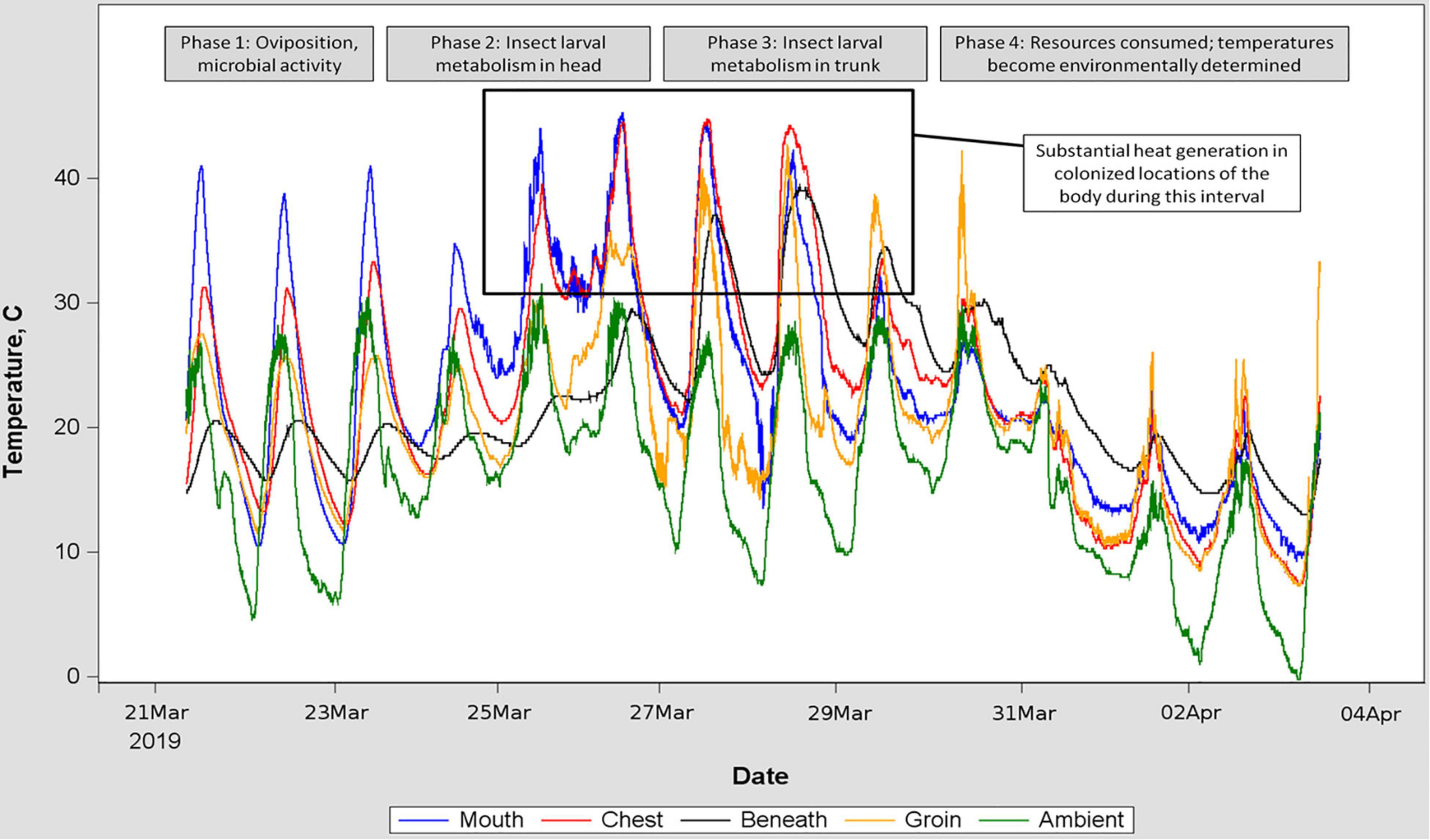
Figure 2. Time series of temperatures recorded by five sensors placed at locations indicated by differently colored traces. Inset text is a hypothetical interpretation of the pattern observed in the temperature traces, and corroborated by in-field observation of the decomposing remains. This placement of porcine remains was chosen for the figure because of the relative consistency of ambient temperature fluctuation, allowing isolation of environmental input from insect heat generation. Blow fly larvae were abundant on the remains between March 25 and March 30.

A DTT value of 0°C was chosen for demonstration of the consequences of biasing DTT relative to a biological limit for development. This value is reported to be used in practice (VanLaerhoven, 2008), and potentially negatively biased values (between 6 and 10°C) are also used for multiple blow fly species (Higley and Haskell, 2001). To investigate the consequences of using Eq. 3 to predict the insect temperatures that would thereafter be used to drive ADD models, we varied the values of parameters C and T_pref naively and again observed resulting changes to the correlation between T_reg and temperature recorded by the relevant thermal probe.

On average, negatively biasing DTT and incorporating thermoregulation both led to improvements in the prediction of larval temperature and ADD, with positive consequences for any application that relies on insect development time estimation. We use individual periods of hog decomposition as examples of what results from changing models, and then summarize the global consequence to prediction using all of our data.

Values to Be Used as T_pref

Temperatures optimal for development, and temperature limits of development, vary by species and life stage (Aubernon et al., 2016; Ahmad and Omar, 2018), but species composition and life stage distributions within the larval communities are not continuously observable in practice. Our model represents a simplification: we used a value of T_pref to use in Equation 3 that was intended to represent an average preferred temperature across species and life stage variation. To estimate this value, we used thermography. We visually delineated (using visible-light versions of photographs) areas in which insects were found, and then statistically summarized the temperatures recorded for those and other areas in a given image. We find that areas in which insects are found (primarily 2nd- and 3rd-instar blow fly larvae) are on average approximately 32°C, both for environments that are warmer than or cooler than that temperature (Figure 3). We interpret this result as an indication that the insects will behaviorally and physiologically act to achieve this temperature, and we used 32°C as a generalized value of T_pref thereafter. The simplification of T_pref used here for the purpose of proving concept in a modeling framework could be specified to relevant species and life stages in application, depending on the species present in a given sample.

FIGURE 3

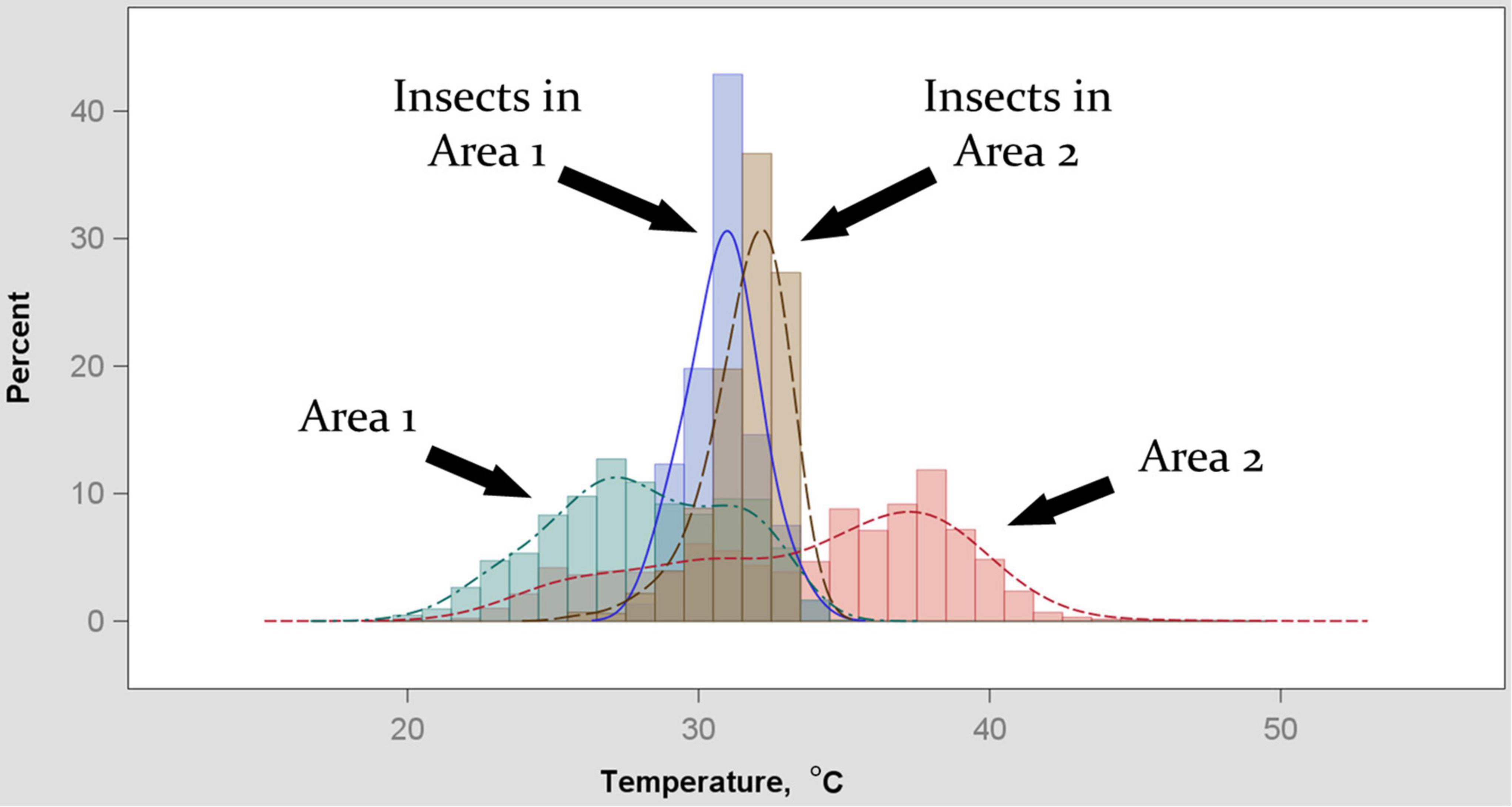
Figure 3. Distributions of temperatures recorded by thermography two areas of decomposing remains. Extent of areas in images was determined by the field-of-view at which larvae could be easily identified in the images, and was approximately 0.25 m². Sub-areas within each image were “Area (1 or 2)” being the extent of remains in the image and “Insects in Area (1 or 2)” being the extent of insect-occupied space within the corresponding area. Dispersion of temperatures for the two larger areas was greater than for the insect-occupied sub-areas. Insect temperature bias was toward an apparent central tendency of 32°C irrespective of whether it resulted in sampling the upper or lower range of the corresponding area.

Shape of Temperature Distributions

Surface temperature distributions from thermographs were similar to slightly positive-skewed normal distributions (Figure 4). For the purpose of this study we decided to model temperatures as normal distributions centered at T_amb. We emphasize that this distributional shape is used for proof of concept and should be investigated for applications to other systems, and suggest that the development of the model framework described here will provide opportunity for such thermal-variation studies of relationships between surface and carrion-mass temperature in blow fly habitats to result in data that can be used by the models to generate improved phenology predictions. Based on this decision we modeled the term P in Eq. 3 as the normal probability distribution function, scaled to have a maximum value of 1, and with a value of 3 for sigma, being low relative to the observed standard deviation of temperature distributions from thermography data and thus a conservative interpretation of the range of temperatures realistically available to insects.

FIGURE 4

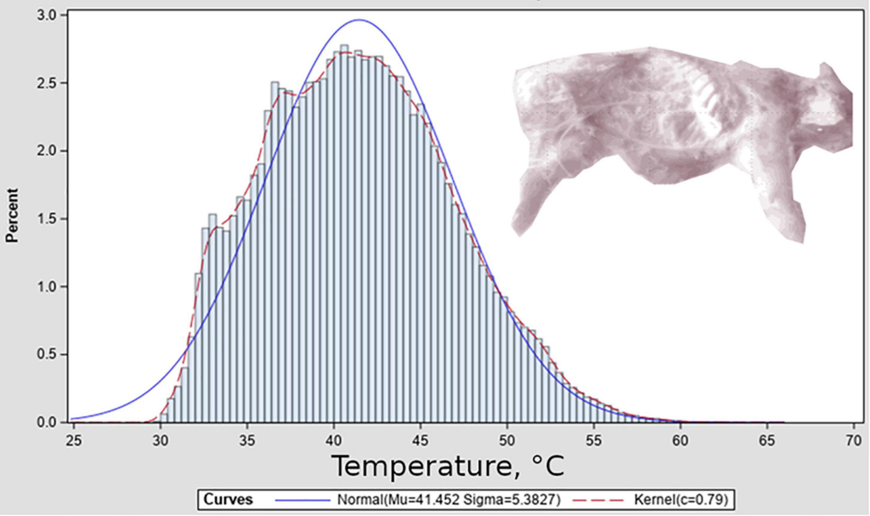
Figure 4. Surface temperature distribution associated with a representative thermograph. Thermograph is shown inset in monochrome, and depicts porcine remains after several days of decomposition; exposed ribs can be seen.

Consequences of Biased Development Threshold Temperature Parameter Values

Biased DTT parameter values can correct for differences between ambient and relevant (taken within or near maggot masses) temperatures in hindsight in two ways. The first is simply because biasing DTT can compensate for bias in temperature recordings. If the average difference between ambient and relevant temperatures is appreciable, then area under the curve for one vs. the other temperature trace will be different in a way that is correctable by adjusting the temperature value equivalent to “zero degree days,” which is the DTT. Decreasing reference against which temperatures are measured to calculate degree-days results in more degree-days per day (Figure 5). The reason this change to DTT works in hindsight and not predictively is that it offsets an accumulation of degree-days (area under the curve) and not necessarily a momentary difference of temperatures. To offset area under the curve, the beginning and end times for the given curve must be known, which is definitively not the case in forensic entomology. In Figure 5, the biased DTT value overcompensates for the temperature difference between ambient and the colonized area in the first 3 days, after which it undercompensates for the subsequent 3 days.

FIGURE 5

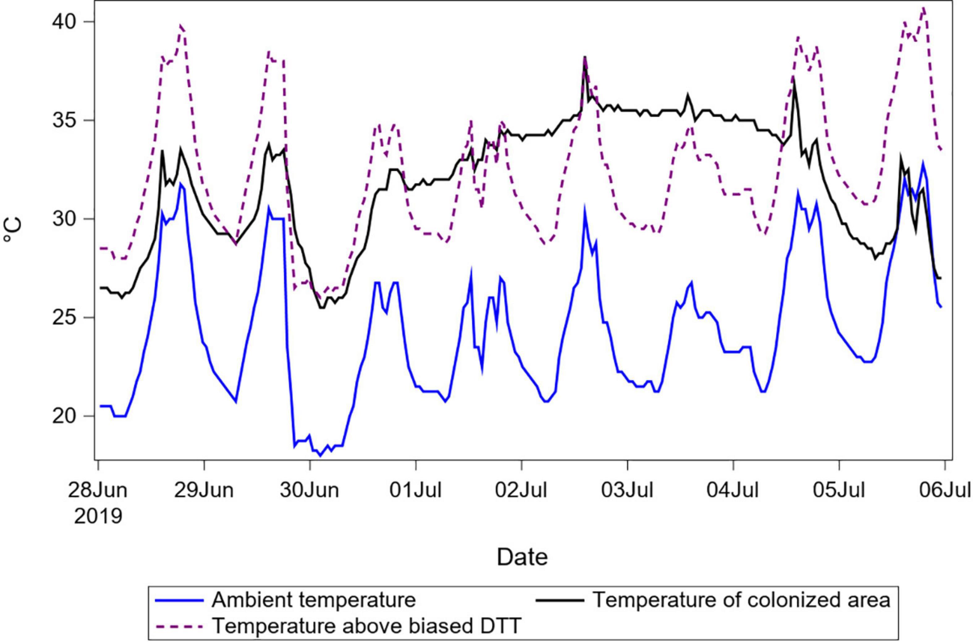
Figure 5. Temperature recordings for porcine remains in summer 2019. Temperatures of ambient air and of the main colonized area of the remains are shown to demonstrate a situation with a consistent difference between these two temperatures through time. Temperature above a (negatively) biased DTT of zero °C is also shown to demonstrate that this bias, equivalent to adding the magnitude of the bias to the ambient temperature, causes the areas under the resulting curve to become close to the area under the curve for temperature of the colonized area. Reducing the DTT results in improved prediction for this case and other cases with similar durations and temperature differences, but not for others.

The second way in which biased DTT parameter values can improve prediction is because decreasing the value of DTT increases the correlation between heat accumulation and time (Figure 6). For example, given a 10-degree change in temperature from 20 to 30 degrees during one time period, a DTT of 10 degrees results in a 100% change in the rate of degree day accumulation (10 above to 20 above the DTT), whereas a DTT of 0 degrees results in a 50% change in the rate of accumulation (20 above to 30 above the DTT). At negatively biased values of DTT, the result is that the degree day accumulation curve is smoothed, and time becomes an increasingly informative predictor of the accumulation of degree days. Conversely, for positively biased values of DTT, time becomes a less informative predictor of DTT. The smoothing outcome of negatively biased DTT also inevitably results in an increase in the absolute value of degree-days accumulated (note the two axes used for Figure 6). If insects thermoregulate to maintain temperature differences relative to ambient and to maintain temperatures that vary less than do ambient temperatures, then these two consequences of biased DTT may both result in improvement for prediction, though with the earlier-mentioned significant caveat of the improvement only applying in hindsight for a known temporal interval, and in situations where ambient temperatures are below insect temperatures.

FIGURE 6

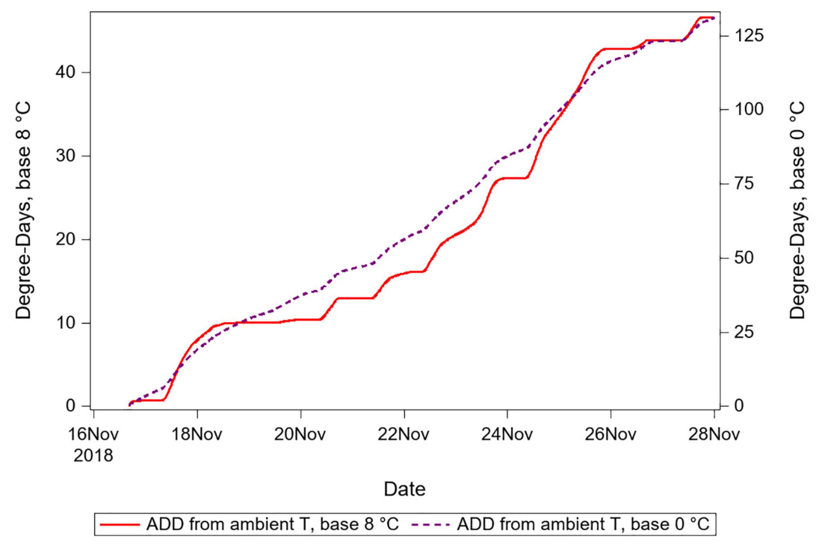
Figure 6. Degree day accumulations calculated using an empirically supported DTT value vs. a value expected to be negatively biased. Note two different Y-axis ranges for each of the two series, which show that ADD calculated using the lower DTT are greater in quantity. The smoothing consequence of reducing proportional variation in degrees-above-DTT is seen in the dashed series, which corresponds to the negatively biased DTT.

Homeothermy Through Thermoregulation Can Increase the Correlation Between Time and Development

Equation 3 represents thermoregulation, with a consequence to distributions of temperature-above-DTT of moving all values toward the organisms’ preferred temperature. Correlations between ambient and predicted temperatures plotted in Figure 7 are similar to Q-Q plots used in fit diagnostics: here, they confirm that the predicted temperatures that assume organisms bias their thermal experience toward some optimum are underdispersed relative to the distribution of ambient temperatures.

FIGURE 7

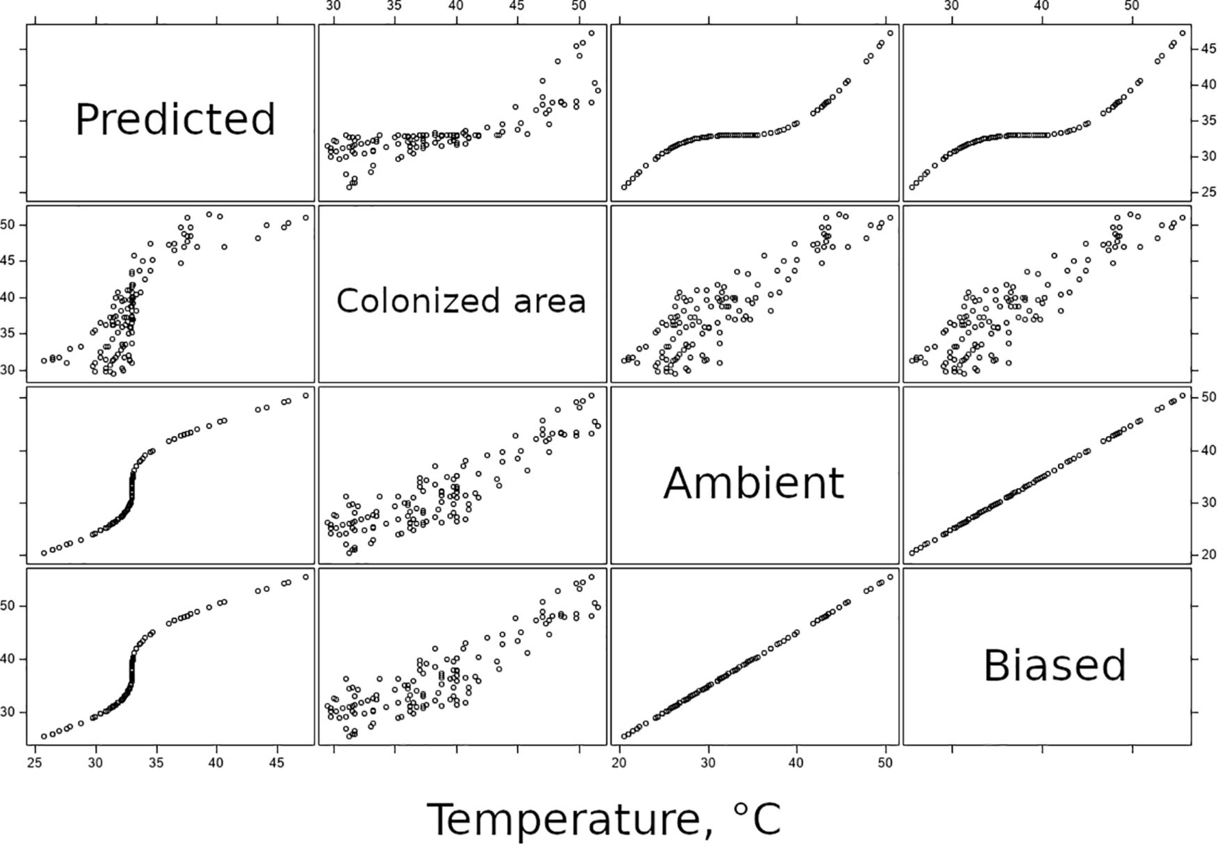
Figure 7. Panel of bivariate correlation plots, relating predicted, colonized area, ambient, and biased-ambient temperatures to each other. Predictions are generated on the basis of ambient temperature; the correlation plots relating these two variables depict the function of Eq. 3 and confirm that the function results in underdispersion relative to the distribution of ambient temperatures.

The observation that biased DTT values can result in strengthened correlation between development and time led us to explore mechanisms through which insects might bias their thermal experience depending upon local conditions. Equation 3 was used to predict the temperature of insects, as a basis for calculating accumulated degree days as would be done with data sourced from networked weather databases (Figure 8). Not only does this derivative temperature estimate improve the fit of predicted to observed degree days, it does so irrespective of whether ambient temperature is above or below preferred temperature. Insect temperature for each time point was predicted as a function of the difference between ambient and preferred temperatures. The function represents the expectation that insects bias their own body temperatures toward preferred temperatures. Insects are relatively more likely to exist at optimal temperature if ambient temperature is relatively nearer optimal, and if temperature variability in remains is relatively higher. As ambient temperature becomes increasingly different from optimal, and variability in remains decreases so that the occurrence of microenvironments near optimal temperatures becomes less likely, insects are expected to have body temperatures nearer to ambient – as is the case in the relatively invariant environments of laboratories in which insects are reared for study of development rate variation at fixed temperatures.

FIGURE 8

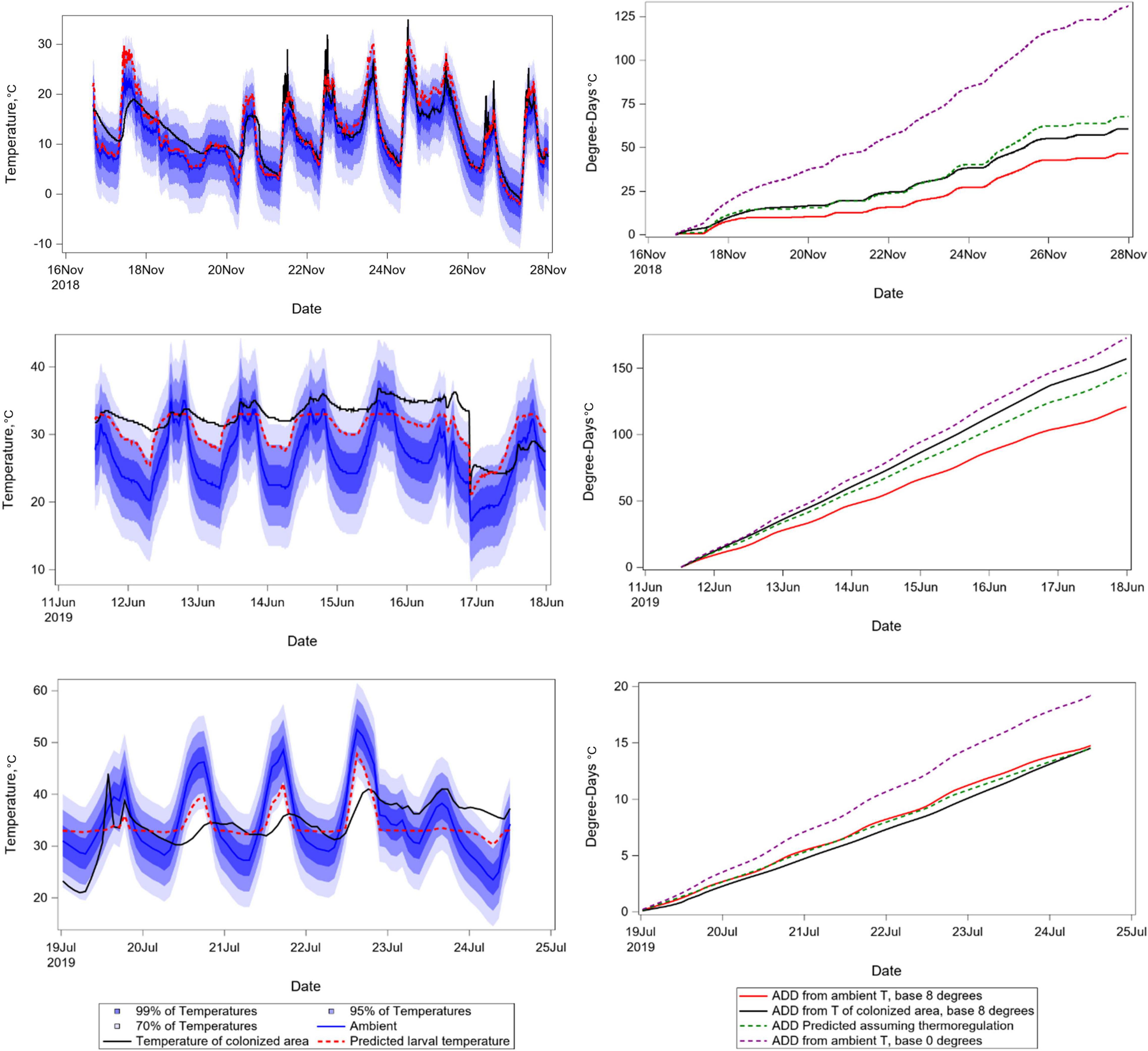
Figure 8. Panel of temperature time series graphs. Left column depicts ambient temperatures, distributions around ambient temperatures assuming variance of 9°C, temperatures recorded from within insect-colonized areas of decomposing remains, and predicted insect larval temperatures generated using Eq. 3 and calculating the value of P assuming normal distributions of temperature around ambient. Right column shows corresponding degree day accumulations resulting from ambient temperatures, predicted temperatures, temperatures recorded from insect-colonized areas, and ambient temperatures but assuming a negatively biased value of DTT. Temporal intervals were chosen to represent relatively cool, moderate, and hot weather.

Biasing DTT and modeling thermoregulation are different mechanisms of correcting for error in the temperature data used to drive phenology models, and the effect of each mechanism as a modulator of ambient temperatures is evident in how each changes the relationship between input and output values (Figure 7). Biasing DTT “moves” a truncated statistical distribution of temperatures up or down, changing the average value of degree days accumulated per unit time. When a distribution of ambient temperatures does not include values below the DTT (as is commonly the case in warm climates), then decreasing the DTT further does not alter the pattern of variation in the distribution at all. In contrast, temperatures determined by thermoregulation may not be correlated with environmental variation at all, as is the case with endotherms or perfect homeotherms.

Histograms of show that the predictive model changes the shape of the distribution of temperatures (Figure 9).

FIGURE 9

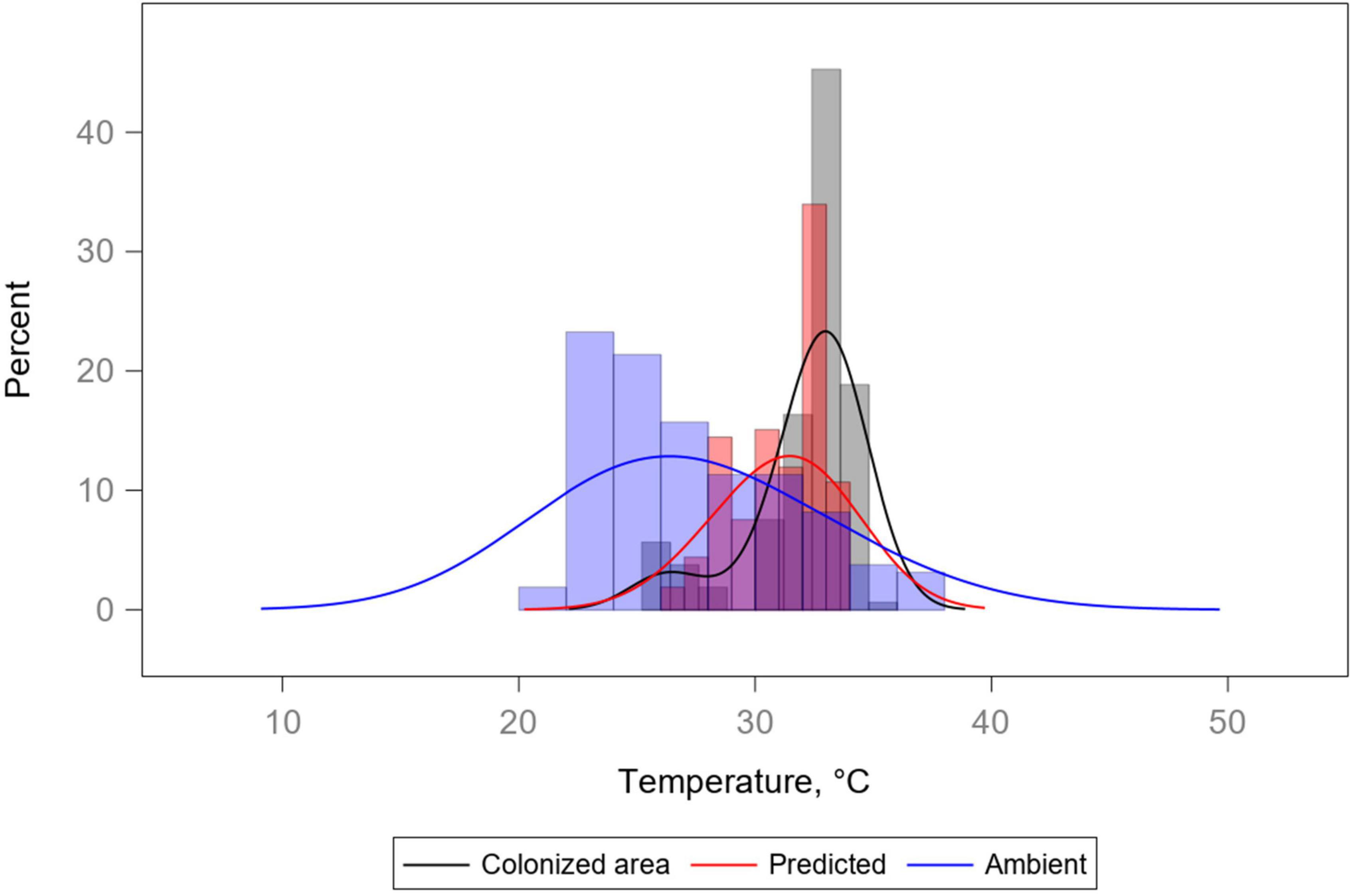
Figure 9. Histograms and kernel density estimate overlays for three temperature variables: colonized area, ambient, and predicted (T_reg) temperatures. Ambient temperature distribution is the most variable of the three, while both the colonized area and the predicted temperature distributions are relatively underdispersed and also tend toward a location different from that of the ambient temperature distribution. Distributions demonstrate how the model is able to generate predictions similar to the “insects in (area 1, 2)” distributions seen in Figure 3.

Overall Improvement in the Accuracy of Temperatures Used in Accumulated Degree-Day Models

Using T_reg as the source of temperature data for calculating ADD improved prediction, when compared to ADD calculations made using ambient temperatures or ambient temperatures with biased DTTs. Using T_reg resulted in movement of the ADD prediction error distribution toward zero, and reduction of the distribution’s variance (Figure 10 and Table 1). Use of a biased DTT (0°C) also improved the error distribution by reducing its variance, but also resulted in greatest average ADD prediction error for our data. For environments where average temperatures are lower than those of south-central Texas, or for biases in DTT less than an 8°C change, predictions involving negatively biased DTTs would be expected to result in less error than they do for our data.

FIGURE 10

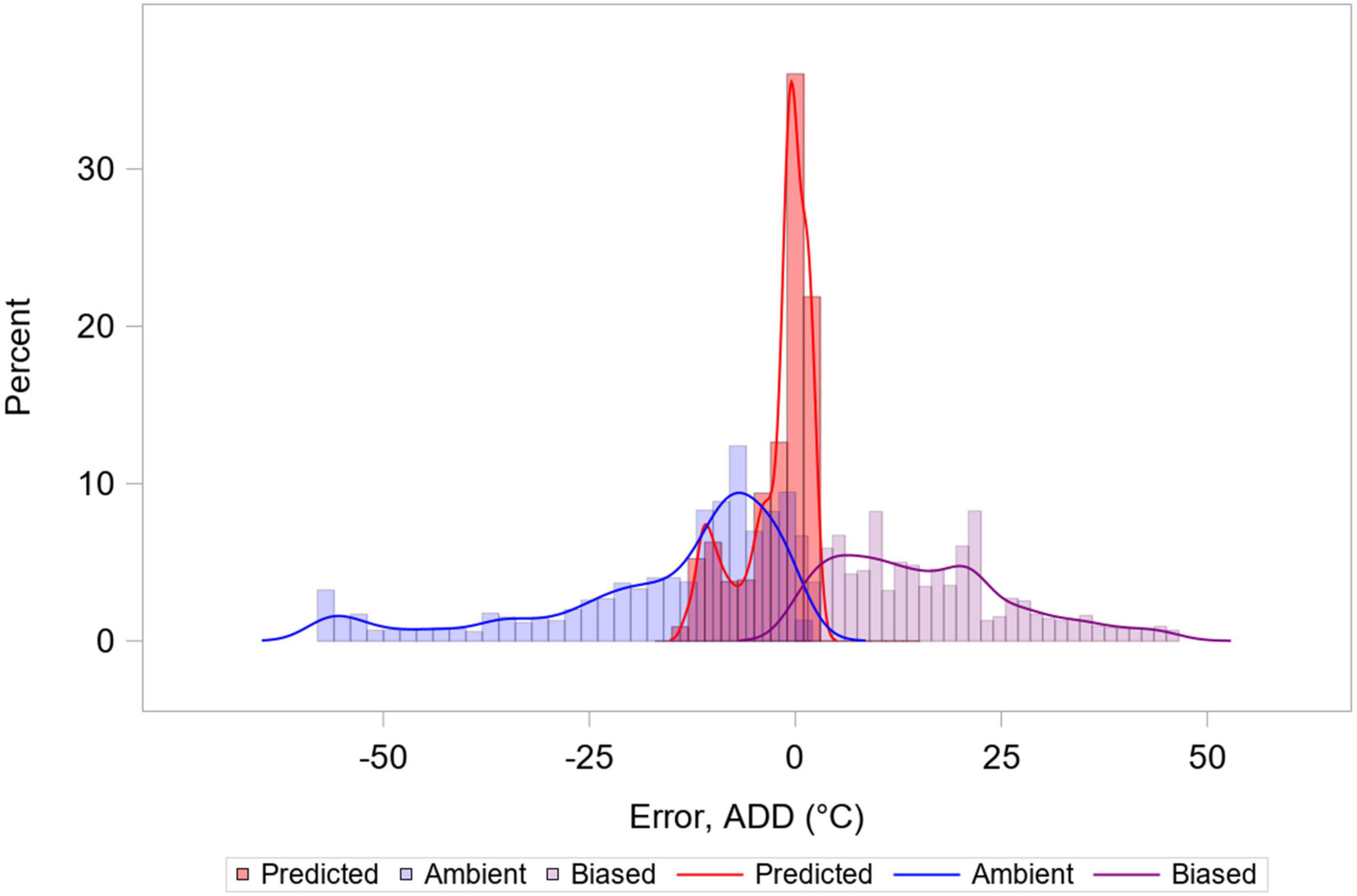
Figure 10. Histograms and kernel density estimate overlays representing three distributions of accumulated degree day (ADD) error. ADD values were calculated from ambient temperatures using the supported development threshold temperature (DTT) of 8°C (Reibe et al., 2010), from ambient temperatures using a biased (0°C) DTT value, and from T_reg from Eq. 3. Calculations using biased DTT lead to reduced range of error, but are biased. Data from 6 hogs are included, and each data point represents one simultaneous temperature recording and derivative ADD value.

TABLE 1

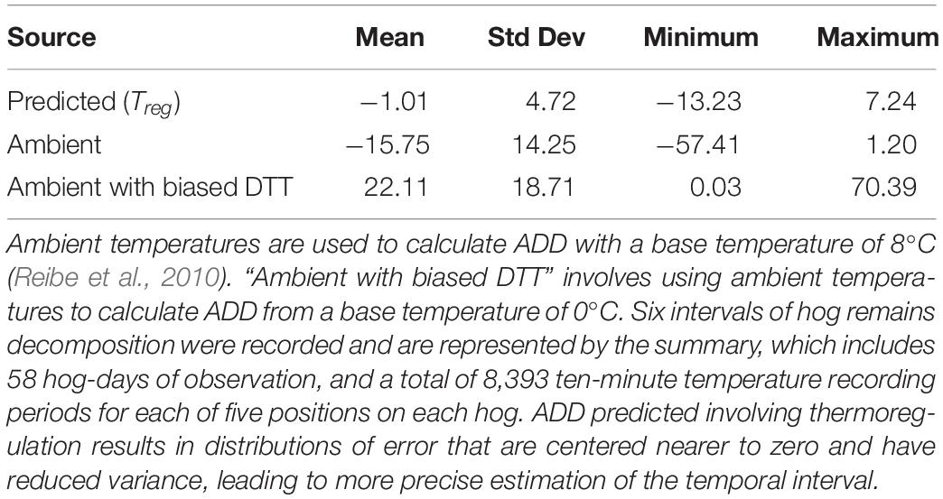
Table 1. Summary of ADD prediction error resulting from the use of different temperature data sources and biased DTT values.

Discussion

This research demonstrates that, while ADD models are useful for capturing environmental variation relevant to phenology, their application becomes more problematic when organisms have a variety of temperatures in their environment from which to “choose” and they regulate their temperatures to an imperfect degree. Blow flies have been demonstrated to meet these criteria (Byrd and Butler, 1996; Huntington et al., 2007; Rivers et al., 2011; Aubernon et al., 2019, 2022). Under these conditions, there are predictable biases in organismal thermal experiences that can be addressed in a few ways. One way to account for partial regulation of temperature is to assume a base temperature that is biased in a way that accounts for bias in the system. This is an unrealistic model from a biological sense, but can create accurate predictions. These results could explain some efforts to assess the best base temperature, where low thresholds have sometimes but not always worked best. One example (VanLaerhoven, 2008) reports the observation that for a blind field validation dataset, that relatively most accurate predictions resulted from using a DTT of 0°C, even though the insects used for estimating time of death have empirically higher base temperatures in lab settings (Anderson, 2000; Núñez–Vázquez et al., 2013). Such an approach leaves a prediction system open to errors. For instance, biases work differently when experienced temperatures are consistently above or below ambient, so deviations from a geographically typical condition can cause challenges for corrected models. Another way to account for this challenge is to algorithmically assume a target temperature (justified by organismal observations) that is sought (not necessarily perfectly) by the organism of interest. This approach is more biologically realistic, involves assumptions that can be empirically confirmed through observation of insects in controlled variable environments, and should in theory be more flexible with respect to thermal fluctuations above and below ambient. We note that the work herein primarily addresses behavioral thermoregulation, because we model insect temperature as a probabilistic function of expected environmental temperatures. A challenge relevant to the forensic entomology discipline and others is that carrion feeding insects themselves can be a source of heat, especially when insects aggregate, meaning there is clear opportunity for insects to experience biased temperatures with respect to ambient temperatures through a mechanism that is dependent on insect heat generation in addition to environmental conditions (Slone and Gruner, 2007; Charabidze et al., 2011; Gruner et al., 2017). Therefore, we advocate further work in this area as we have demonstrated the potential for success with this approach.

Our results illustrate an issue with modeling: correlative methods to estimate parameter values in phenology models are commonly realized as generalized linear modeling approaches that do not incorporate context dependence of the modeled process. Phenology models are typically driven by environmental factors and are thus inherently context-dependent, but the assumption that environment is experienced randomly ignores the importance of behavior in determining which values of environmental variables across heterogeneous spaces should be expected to be driving the realized developmental process. The reason that thermoregulation-based predictions derived from ambient temperatures improve the fit of degree-day accumulation to that calculated from temperatures recorded directly from colonized areas is not because the predictions result in temperature predictions that are highly correlated with those of insects. Figure 8 shows that predicted and colonized area temperatures can in fact be “out of phase” with respect to diurnal cycles. These “out of phase” relationships between diurnal ambient and diurnal insect temperatures are possible and could be uncorrelated or could even have strong negative correlations, potentially for biological reasons such as exploiting the thermal inertia of a solar-irradiated microenvironment to maintain body temperature while also assimilating nutritional resources (Aubernon et al., 2019). The reason that the thermoregulation-based predictions improve ADD calculations in comparison to the “true” ADD values calculated from colonized area temperatures is that the predictions bring the average and variation of the predicted temperature distribution into line with reality. This improvement results whether conditions are hot or cold relative to average, or temperatures are above or below organisms’ preferred values, and can be made through a process that is both intuitively sound and empirically substantiated: the organisms sample environmental temperature distributions non-randomly, and tend toward values that improve fitness and survival (Aubernon et al., 2016; Podhorna et al., 2018).

This research was targeted toward a specific example: carrion feeding insects whose developmental states are important to forensic entomology casework. This system is a good starting point, as the system is rife with thermal variation in time and space, attached to important issues for application of accurate evidence for justice, and is associated with important ecological processes (decomposition, nutrient recycling). As noted above, the observations in the system also appear to support the important aspects of the modeling conditions – including the base temperature offset discussed herein. However, the model should be evaluated under different environmental conditions (for example at low temperatures).

Forensic entomology has a need to validate results predicted from phenology models. A result of this need is that the field has produced observations that address concerns of relevance to all that implement accumulated degree models for phenology research or applications. The field has demonstrated that cold-biased DTT values that seem biologically unrealistic can appear to provide good field-based predictions. The work presented here suggests that unrealistic parameter values increase predictive performance because of an issue with the models: the increased correlation between heat accumulation and time is not due to carrion-feeding flies’ being able to develop at temperatures lower than empirically confirmed minima, but because the flies regulate their temperatures in the face of environmental variation through behavior and physiology. Here, we present a means of accounting for such thermal regulation within the bounds of a traditional accumulated degree model and explore how this compares to use of a biased DTT. We conclude that incorporating regulation into ADD models is a more realistic and robust way to advance these models. Thus, we provide a means to account for thermal regulation in ADD models, and expect that this means enhances applicability of ADD models across a variety of systems in which subject insects partially regulate the temperatures on which their development depends. The field of forensic entomology is poised to help address such issues and in rigorous testing of this and similar models, may be able to help a variety of fields advance their understanding of how organismal behavior impacts and can be incorporated into thermally driven phenology models.

Data Availability Statement

The raw data supporting the conclusions of this article will be made available by the authors, without undue reservation.

Ethics Statement

Ethical review and approval was not required for study involving deceased human participants in accordance with legislation and institutional requirements. Written informed consent for participation by deceased humans was not required for this study in accordance with legislation and institutional requirements. Ethical review and approval was not required for the animal study because animals were deceased at the time of acquisition and the Texas A&M University Institutional Animal Care and Use Committee thus required no animal use protocol.

Author Contributions

TC, AT, and TR contributed to conception and design of the study, conducted fieldwork, and developed the model framework. TR collected the thermal images. TC wrote the manuscript. All authors contributed to manuscript revision, read, and approved the submitted version.

Funding

This research was supported by the National Institute of Justice grant #2016-DN-BX-0204 and USDA-NIFA Hatch Project #TEX09705.

Conflict of Interest

The authors declare that the research was conducted in the absence of any commercial or financial relationships that could be construed as a potential conflict of interest.

Publisher’s Note

All claims expressed in this article are solely those of the authors and do not necessarily represent those of their affiliated organizations, or those of the publisher, the editors and the reviewers. Any product that may be evaluated in this article, or claim that may be made by its manufacturer, is not guaranteed or endorsed by the publisher.

Acknowledgments

We thank The Forensic Anthropology Center at Texas State for allowing our observation of human remains in the field, and Daniel Wescott for thoughtful discussions and for facilitating our visits to the FACTS. We thank the landowners who provided hog remains to us for research. We thank Jeff Tomberlin for facilitating hog storage and transport logistics, and for guidance on insect observation. The Ecology and Natural Resources Teaching Area of Texas A&M University is gratefully acknowledged for use of field sites for hog placement and observation.

References

Addeo, N. F., Li, C., Rusch, T. W., Dickerson, A. J., Tarone, A. M., Bovera, F., et al. (2021). Impact of age, size, and sex on adult black soldier fly [Hermetia illucens L. (Diptera: Stratiomyidae)] thermal preference. J. Insects Food Feed 8, 129–139. doi: 10.3920/jiff2021.0076

PubMed Abstract | CrossRef Full Text | Google Scholar

Ahmad, A., and Omar, B. (2018). Effect of carcass model on maggot distribution and thermal generation of two forensically important blowfly species, Chrysomya megacephala (Fabricius) and Chrysomya rufifacies (Macquart). Egypt. J. Forensic Sci. 8:64.

Google Scholar

Amendt, J., Campobasso, C. P., Gaudry, E., Reiter, C., LeBlanc, H. N., and Hall, M. J. (2007). Best practice in forensic entomology—standards and guidelines. Int. J. Legal Med. 121, 90–104. doi: 10.1007/s00414-006-0086-x

PubMed Abstract | CrossRef Full Text | Google Scholar

Ames, C., and Turner, B. (2003). Low temperature episodes in development of blowflies: implications for postmortem interval estimation. Med. Vet. Entomol. 17, 178–186. doi: 10.1046/j.1365-2915.2003.00421.x

PubMed Abstract | CrossRef Full Text | Google Scholar

Anderson, G. S. (2000). Minimum and maximum development rates of some forensically important Calliphoridae (Diptera). J. Forensic Sci. 45, 824–832.

PubMed Abstract | Google Scholar

Angilletta, M. J. Jr. (2009). Thermal Adaptation: A Theoretical and Empirical Synthesis. Oxford: Oxford University Press.

Google Scholar

Archer, M. S. (2004). The effect of time after body discovery on the accuracy of retrospective weather station ambient temperature corrections in forensic entomology. J. Forensic Sci. 49, 1–7. doi: 10.1520/jfs2003258

PubMed Abstract | CrossRef Full Text | Google Scholar

Archer, M. S., and Elgar, M. A. (2003). Female breeding-site preferences and larval feeding strategies of carrion-breeding Calliphoridae and Sarcophagidae (Diptera): a quantitative analysis. Aust. J. Zool. 51, 165–174. doi: 10.1071/zo02067

CrossRef Full Text | Google Scholar

Aubernon, C., Boulay, J., Hédouin, V., and Charabidzé, D. (2016). Thermoregulation in gregarious dipteran larvae: evidence of species-specific temperature selection. Entomol. Exp. Appl. 160, 101–108. doi: 10.1111/eea.12468

CrossRef Full Text | Google Scholar

Aubernon, C., Fouche, Q., and Charabidze, D. (2022). Developmental niche construction in necrophagous larval societies: feeding facilitation can offset the costs of low ambient temperature. Ecol. Entomol. 1–9.

Google Scholar

Aubernon, C., Hedouin, V., and Charabidze, D. (2019). The maggot, the ethologist and the forensic entomologist: sociality and thermoregulation in necrophagous larvae. J. Adv. Res. 16, 67–73. doi: 10.1016/j.jare.2018.12.001

PubMed Abstract | CrossRef Full Text | Google Scholar

Baqué, M., and Amendt, J. (2013). Strengthen forensic entomology in court—the need for data exploration and the validation of a generalised additive mixed model. Int. J. Legal Med. 127, 213–223. doi: 10.1007/s00414-012-0675-9

PubMed Abstract | CrossRef Full Text | Google Scholar

Barton, P. S., Dawson, B. M., Barton, A. F., Joshua, S., and Wallman, J. F. (2021). Temperature dynamics in different body regions of decomposing vertebrate remains. Forensic Sci. Int. 325:110900.

Google Scholar

Boatright, S. A., and Tomberlin, J. K. (2010). Effects of temperature and tissue type on the development of Cochliomyia macellaria (Diptera: Calliphoridae). J. Med. Entomol. 47, 917–923. doi: 10.1093/jmedent/47.5.917

CrossRef Full Text | Google Scholar

Byrd, J. H., and Butler, J. F. (1996). Effects of temperature on Cochliomyia macellaria (Diptera: Calliphoridae) development. J. Med. Entomol. 33, 901–905. doi: 10.1093/jmedent/33.6.901

PubMed Abstract | CrossRef Full Text | Google Scholar

Byrd, J. H., and Tomberlin, J. K. (eds). (2019). Forensic Entomology: The Utility of Arthropods in Legal Investigations. Boca Raton, FL: CRC Press, 213–224.

Google Scholar

Catts, E. P. (1992). Problem in estimating the postmortem interval in death investigations. J. Agric. Entomol. 9, 245–255.

Google Scholar

Catts, E. P., and Goff, M. L. (1992). Forensic entomology in criminal investigations. Annu. Rev. Entomol. 37, 253–272. doi: 10.1146/annurev.en.37.010192.001345

PubMed Abstract | CrossRef Full Text | Google Scholar

Catts, E. P., and Haskell, N. H. (eds). (1990). Entomology and Death: A Procedural Guide. Clemson, SC: Joyce’s Print Shop.

Google Scholar

Cervantès, L., Dourel, L., Gaudry, E., Pasquerault, T., and Vincent, B. (2017). Effect of low temperature in the development cycle of Lucilia sericata (Meigen) (Diptera, Calliphoridae): implications for the minimum postmortem interval estimation. Forensic Sci. Res. 3, 52–59. doi: 10.1080/20961790.2017.1406839

PubMed Abstract | CrossRef Full Text | Google Scholar

Chappell, T. M., Beaudoin, A. L., and Kennedy, G. G. (2013). Interacting virus abundance and transmission intensity underlie tomato spotted wilt virus incidence: an example weather-based model for cultivated tobacco. PLoS One 8:e73321. doi: 10.1371/journal.pone.0073321

PubMed Abstract | CrossRef Full Text | Google Scholar

Chappell, T. M., Ward, R. V., DePolt, K. T., Roberts, P. M., Greene, J. K., and Kennedy, G. G. (2020). Cotton thrips infestation predictor: a practical tool for predicting tobacco thrips (Frankliniella fusca) infestation of cotton seedlings in the south-eastern United States. Pest Manag. Sci. 76, 4018–4028. doi: 10.1002/ps.5954

PubMed Abstract | CrossRef Full Text | Google Scholar

Charabidze, D., Bourel, B., and Gosset, D. (2011). Larval-mass effect: characterisation of heat emission by necrophageous blowflies (Diptera: Calliphoridae) larval aggregates. Forensic Sci. Int. 211, 61–66. doi: 10.1016/j.forsciint.2011.04.016

PubMed Abstract | CrossRef Full Text | Google Scholar

Charabidze, D., and Hedouin, V. (2019). Temperature: the weak point of forensic entomology. Int. J. Legal Med. 133, 633–639.

Google Scholar

Crimmins, T. M., Gerst, K. L., Huerta, D. G., Marsh, R. L., Posthumus, E. E., Rosemartin, A. H., et al. (2020). Short-term forecasts of insect phenology inform pest management. Ann. Entomol. Soc. Am. 113, 139–148. doi: 10.1093/aesa/saz026

PubMed Abstract | CrossRef Full Text | Google Scholar

Dabbs, G. R. (2015). How should forensic anthropologists correct national weather service temperature data for use in estimating the postmortem interval? J. Forensic Sci. 60, 581–587. doi: 10.1111/1556-4029.12724

PubMed Abstract | CrossRef Full Text | Google Scholar

Day, T., and Rowe, L. (2002). Developmental thresholds and the evolution of reaction norms for age and size at life-history transitions. Am. Nat. 159, 338–350. doi: 10.1086/338989

PubMed Abstract | CrossRef Full Text | Google Scholar

Dourel, L., Pasquerault, T., Gaudry, E., and Vincent, B. (2010). Using estimated on-site ambient temperature has uncertain benefit when estimating postmortem interval. Psyche 2010, 1–7. doi: 10.1155/2010/610639

CrossRef Full Text | Google Scholar

Faigman, D. (2002). Science and the law: is science different for lawyers? Science 297, 339–340. doi: 10.1126/science.1072515

PubMed Abstract | CrossRef Full Text | Google Scholar

Flores, M. (2013). Life-History Traits of Chrysomya rufifacies (Macquart) (Diptera: Calliphoridae) and its Associated Non-Consumptive Effects on Cochliomyia macellaria (Fabricius) (Diptera: Calliphoridae) Behavior and Development. Doctoral dissertation. College Station, TX: Texas A & M University.

Google Scholar

Gallagher, M. B., Sandhu, S., and Kimsey, R. (2010). Variation in developmental time for geographically distinct populations of the common green bottle fly, Lucilia sericata (Meigen). J. Forensic Sci. 55, 438–442. doi: 10.1111/j.1556-4029.2009.01285.x

PubMed Abstract | CrossRef Full Text | Google Scholar

Gaudry, E., and Dourel, L. (2013). Forensic entomology: implementing quality assurance for expertise work. Int. J. Legal Med. 127, 1031–1037.

Google Scholar

Gelderman, T., Stigter, E., Krap, T., Amendt, J., and Duijst, W. (2021). The time of death in Dutch court; using the Daubert criteria to evaluate methods to estimate the PMI used in court. Legal Med. 53:101970.

Google Scholar

Gould, S. J. (1992). Bully for Brontosaurus: Reflections in Natural History. New York, NY: WW Norton and Company, 463–472.

Google Scholar

Grassberger, M., and Reiter, C. (2001). Effect of temperature on Lucilia sericata (Diptera: Calliphoridae) development with special reference to the isomegalen- and isomorphen-diagram. Forensic Sci. Int. 120, 32–36. doi: 10.1016/s0379-0738(01)00413-3

PubMed Abstract | CrossRef Full Text | Google Scholar

Grassberger, M., and Reiter, C. (2002a). Effect of temperature on development of Liopygia (= Sarcophaga) argyrostoma (Robineau-Desvoidy) (Diptera: Sarcophagidae) and its forensic implications. J. Forensic Sci. 47, 1332–1336.

PubMed Abstract | Google Scholar

Grassberger, M., and Reiter, C. (2002b). Effect of temperature on development of the forensically important holarctic blowfly Protophormia terraenovae (Robineau-Desvoidy) (Diptera: Calliphoridae). Forensic Sci. Int. 128, 177–182. doi: 10.1016/s0379-0738(02)00199-8

PubMed Abstract | CrossRef Full Text | Google Scholar

Gruner, S. V., Slone, D. H., Capinera, J. L., and Turco, M. P. (2017). Volume of larvae is the most important single predictor of mass temperatures in the forensically important calliphorid, Chrysomya megacephala (Diptera: Calliphoridae). J. Med. Entomol. 54, 30–34. doi: 10.1093/jme/tjw139

PubMed Abstract | CrossRef Full Text | Google Scholar

Harnden, L. M., and Tomberlin, J. K. (2016). Effects of temperature and diet on black soldier fly, Hermetia illucens (L.) (Diptera: Stratiomyidae), development. Forensic Sci. Int. 266, 109–116. doi: 10.1016/j.forsciint.2016.05.007

PubMed Abstract | CrossRef Full Text | Google Scholar

Heaton, V., Moffatt, C., and Simmons, T. (2014). Quantifying the temperature of maggot masses and its relationship to decomposition. J. Forensic Sci. 59, 676–682. doi: 10.1111/1556-4029.12396

PubMed Abstract | CrossRef Full Text | Google Scholar

Heaton, V., Moffatt, C., and Simmons, T. (2018). The movement of fly (Diptera) larvae within a feeding aggregation. Can. Entomol. 150, 326–333.

Google Scholar

Higley, L. G., and Haskell, N. H. (2001). Insect Development and Forensic Entomology. Forensic Entomology: The Utility of Arthropods in Legal Investigations. Boca Raton, FL: CRC Press.

Google Scholar

Huntington, T. E., Higley, L. G., and Baxendale, F. P. (2007). Maggot development during morgue storage and its effect on estimating the post-mortem interval. J. Forensic Sci. 52, 453–458. doi: 10.1111/j.1556-4029.2007.00385.x

PubMed Abstract | CrossRef Full Text | Google Scholar

Ikemoto, T. (2005). Intrinsic optimum temperature for development of insects and mites. Environ. Entomol. 34, 1377–1387. doi: 10.1603/EN12058

PubMed Abstract | CrossRef Full Text | Google Scholar

Ikemoto, T., and Egami, C. (2013). Mathematical elucidation of the Kaufmann effect based on the thermodynamic SSI model. Appl. Entomol. Zool. 48, 313–323. doi: 10.1007/s13355-013-0190-6

CrossRef Full Text | Google Scholar

Ikemoto, T., and Takai, K. (2000). A new linearized formula for the law of total effective temperature and the evaluation of line-fitting methods with both variables subject to error. Environ. Entomol. 29, 671–682. doi: 10.1603/0046-225x-29.4.671

PubMed Abstract | CrossRef Full Text | Google Scholar

Jensen, J. L. W. V. (1906). Sur les fonctions convexes et les inégalités entre les valeurs moyennes. Acta Math. 30, 175–193. doi: 10.1007/bf02418571

CrossRef Full Text | Google Scholar

Johnson, A. P., Wighton, S. J., and Wallman, J. F. (2014). Tracking movement and temperature selection of larvae of two forensically important blow fly species within a “maggot mass”. J. Forensic Sci. 59, 1586–1591. doi: 10.1111/1556-4029.12472

PubMed Abstract | CrossRef Full Text | Google Scholar

Kaspari, M. (2019). In a globally warming world, insects act locally to manipulate their own microclimate. Proc. Natl. Acad. Sci. U.S.A. 116, 5220–5222. doi: 10.1073/pnas.1901972116

PubMed Abstract | CrossRef Full Text | Google Scholar

Kaufmann, O. (1932). Einige bemerkungen über den Einfluß von temperaturschwankungen auf die entwicklungsdauer und streuung bei Insekten und seine graphische darstellung durch kettenlinie und hyperbel. Z. Morphol. Ökol. Tiere 25, 354–361.

Google Scholar

Kemp, W. P., Dennis, B., and Beckwith, R. C. (1986). Stochastic phenology model for the western spruce budworm (Lepidoptera: Tortricidae). Environ. Entomol. 15, 547–554. doi: 10.1093/ee/15.3.547

PubMed Abstract | CrossRef Full Text | Google Scholar

Lamb, R. J. (1992). Developmental rate of Acyrthosiphon pisum (Homoptera: Aphididae) at low temperatures: implications for estimating rate parameters for insects. Environ. Entomol. 21, 10–19. doi: 10.1093/ee/21.1.10

CrossRef Full Text | Google Scholar

Lamb, R. J., Gerber, G. H., and Atkinson, G. F. (1984). Comparison of developmental rate curves applied to egg hatching data of Entomoscelis americana Brown (Coleoptera: Chrysomelidae). Environ. Entomol. 13, 868–872. doi: 10.1093/ee/13.3.868

CrossRef Full Text | Google Scholar

Martin, T. L., and Huey, R. B. (2008). Why “suboptimal” is optimal: Jensen’s inequality and ectotherm thermal preferences. Am. Nat. 171, 102–118. doi: 10.1086/527502

PubMed Abstract | CrossRef Full Text | Google Scholar

Matuszewski, S. (2011). Estimating the pre-appearance interval from temperature in Necrodes littoralis L.(Coleoptera: Silphidae). Forensic Sci. Int. 212, 180–188. doi: 10.1016/j.forsciint.2011.06.010

PubMed Abstract | CrossRef Full Text | Google Scholar

Matuszewski, S. (2021). Post-mortem interval estimation based on insect evidence: current challenges. Insects 12:314. doi: 10.3390/insects12040314

PubMed Abstract | CrossRef Full Text | Google Scholar

Matuszewski, S., and Mądra-Bielewicz, A. (2016). Validation of temperature methods for the estimation of pre-appearance interval in carrion insects. Forensic Sci. Med. Pathol. 12, 50–57. doi: 10.1007/s12024-015-9735-z

PubMed Abstract | CrossRef Full Text | Google Scholar

Michaud, J. P., and Moreau, G. (2011). A statistical approach based on accumulated degree-days to predict decomposition-related processes in forensic studies. J. Forensic Sci. 56, 229–232. doi: 10.1111/j.1556-4029.2010.01559.x

PubMed Abstract | CrossRef Full Text | Google Scholar

Núñez–Vázquez, C., Tomberlin, J. K., Cantú–Sifuentes, M., and García–Martínez, O. (2013). Laboratory development and field validation of Phormia regina (Diptera: Calliphoridae). J. Med. Entomol. 50, 252–260. doi: 10.1603/me12114

PubMed Abstract | CrossRef Full Text | Google Scholar

OSAC (2021). Work Products. Organizational of Scientific Area Committees for Forensic Science. Gaithersburg, MD: National Institute of Standards and Technology.

Google Scholar

Pincebourde, S., and Casas, J. (2019). Narrow safety margin in the phyllosphere during thermal extremes. Proc. Natl. Acad. Sci. U.S.A. 116, 5588–5596. doi: 10.1073/pnas.1815828116

PubMed Abstract | CrossRef Full Text | Google Scholar

Podhorna, J., Aubernon, C., Borkovcova, M., Boulay, J., Hedouin, V., and Charabidze, D. (2018). To eat or get heat: behavioral trade-offs between thermoregulation and feeding in gregarious necrophagous larvae. Insect Sci. 25, 883–893. doi: 10.1111/1744-7917.12465

PubMed Abstract | CrossRef Full Text | Google Scholar

Post, E. (2019). Time in Ecology. Princeton, NJ: Princeton University Press, 15–43.

Google Scholar

Reibe, S., Doetinchem, P. V., and Madea, B. (2010). A new simulation-based model for calculating post-mortem intervals using developmental data for Lucilia sericata (Dipt.: Calliphoridae). Parasitol. Res. 107, 9–16. doi: 10.1007/s00436-010-1879-x

PubMed Abstract | CrossRef Full Text | Google Scholar

Rivers, D. B., Thompson, C., and Brogan, R. (2011). Physiological trade-offs of forming maggot masses by necrophagous flies on vertebrate carrion. Bull. Entomol. Res. 101, 599–611.

Google Scholar

Sanford, M. R., Byrd, J. H., Tomberlin, J. K., and Wallace, J. R. (2019). “Entomological evidence collections methods: american board of forensic entomology approved protocols,” in Forensic Entomology: The Utility of Arthropods in Legal Investigations, eds J. H. Byrd and J. K. Tomberlin (Boca Raton, FL: CRC Press), 63–85. doi: 10.4324/9781351163767-3

CrossRef Full Text | Google Scholar

Saunders, D. S., and Hayward, S. A. (1998). Geographical and diapause-related cold tolerance in the blow fly, Calliphora vicina. J. Insect Physiol. 44, 541–551. doi: 10.1016/s0022-1910(98)00049-3

PubMed Abstract | CrossRef Full Text | Google Scholar

Schoolfield, R. M., Sharpe, P. J. H., and Magnuson, C. E. (1981). Non-linear regression of biological temperature-dependent rate models based on absolute reaction-rate theory. J. Theor. Biol. 88, 719–731. doi: 10.1016/0022-5193(81)90246-0

PubMed Abstract | CrossRef Full Text | Google Scholar

Sharpe, P. J., and DeMichele, D. W. (1977). Reaction kinetics of poikilotherm development. J. Theor. Biol. 64, 649–670. doi: 10.1016/0022-5193(77)90265-x

CrossRef Full Text | Google Scholar

Singer, M. C., and Parmesan, C. (2010). Phenological asynchrony between herbivorous insects and their hosts: signal of climate change or pre-existing adaptive strategy? Philos. Trans. R. Soc. B Biol. Sci. 365, 3161–3176. doi: 10.1098/rstb.2010.0144

PubMed Abstract | CrossRef Full Text | Google Scholar

Slone, D. H., and Gruner, S. V. (2007). Thermoregulation in larval aggregations of carrion-feeding blow flies (Diptera: Calliphoridae). J. Med. Entomol. 44, 516–523. doi: 10.1603/0022-2585(2007)44[516:tilaoc]2.0.co;2

PubMed Abstract | CrossRef Full Text | Google Scholar

Stinner, R. E., Gutierrez, A. P., and Butler, G. D. (1974). An algorithm for temperature-dependent growth rate simulation. Can. Entomol. 106, 519–524. doi: 10.4039/ent106519-5

CrossRef Full Text | Google Scholar

Tarone, A. M., and Foran, D. R. (2008). Generalized additive models and Lucilia sericata growth: assessing confidence intervals and error rates in forensic entomology. J. Forensic Sci. 53, 942–948. doi: 10.1111/j.1556-4029.2008.00744.x

PubMed Abstract | CrossRef Full Text | Google Scholar

Tarone, A. M., Picard, C. J., Spiegelman, C., and Foran, D. R. (2011). Population and temperature effects on Lucilia sericata (Diptera: Calliphoridae) body size and minimum development time. J. Med. Entomol. 48, 1062–1068. doi: 10.1603/me11004

PubMed Abstract | CrossRef Full Text | Google Scholar

Tarone, A. M., and Sanford, M. R. (2017). Is PMI the hypothesis or the null hypothesis? J. Med. Entomol. 54, 1109–1115. doi: 10.1093/jme/tjx119

PubMed Abstract | CrossRef Full Text | Google Scholar

Tobin, P. C., Nagarkatti, S., Loeb, G., and Saunders, M. C. (2008). Historical and projected interactions between climate change and insect voltinism in a multivoltine species. Glob. Chang. Biol. 14, 951–957. doi: 10.1111/j.1365-2486.2008.01561.x

CrossRef Full Text | Google Scholar

Turner, B., and Howard, T. (1992). Metabolic heat generation in dipteran larval aggregations: a consideration for forensic entomology. Med. Vet. Entomol. 6, 179–181. doi: 10.1111/j.1365-2915.1992.tb00602.x

PubMed Abstract | CrossRef Full Text | Google Scholar

VanLaerhoven, S. L. (2008). Blind validation of postmortem interval estimates using developmental rates of blow flies. Forensic Sci. Int. 180, 76–80. doi: 10.1016/j.forsciint.2008.07.002

PubMed Abstract | CrossRef Full Text | Google Scholar

Wagner, T. L., Wu, H. I., Sharpe, P. J., Schoolfield, R. M., and Coulson, R. N. (1984). Modeling insect development rates: a literature review and application of a biophysical model. Ann. Entomol. Soc. Am. 77, 208–220. doi: 10.1093/aesa/77.2.208

CrossRef Full Text | Google Scholar

Worner, S. P. (1992). Performance of phenological models under variable temperature regimes: consequences of the Kaufmann or rate summation effect. Environ. Entomol. 21, 689–699. doi: 10.1093/ee/21.4.689

PubMed Abstract | CrossRef Full Text | Google Scholar