A Convolutional Neural Network Bird Species Recognizer Built From Little Data by Iteratively Training, Detecting, and Labeling

Automatically detecting the calls of species of interest in audio recordings is a common but often challenging exercise in ecoacoustics. This challenge is increasingly being tackled with deep neural networks that generally require a rich set of training data. Often, the available training data might not be from the same geographical region as the study area and so may contain important differences. This mismatch in training and deployment datasets can impact the accuracy at deployment, mainly due to confusing sounds absent from the training data generating false positives, as well as some variation in call types. We have developed a multiclass convolutional neural network classifier for seven target bird species to track presence absence of these species over time in cotton growing regions. We started with no training data from cotton regions but we did have an unbalanced library of calls from other locations. Due to the relative scarcity of calls in recordings from cotton regions, manually scanning and labeling the recordings was prohibitively time consuming. In this paper we describe our process of overcoming this data mismatch to develop a recognizer that performs well on the cotton recordings for most classes. The recognizer was trained on recordings from outside the cotton regions and then applied to unlabeled cotton recordings. Based on the resulting outputs a verification set was chosen to be manually tagged and incorporated in the training set. By iterating this process, we were gradually able to build the training set of cotton audio examples. Through this process, we were able to increase the average class F1 score (the harmonic mean of precision and recall) of the recognizer on target recordings from 0.45 in the first iteration to 0.74.

Introduction

Surveys of birds belonging to various functional groups over time can give farmers information about the health of the ecosystems on their farms. It is in the interest of cotton farmers to improve biodiversity and ecosystem function on their farms: healthy ecosystems may improve productivity of the farms in the long term through pest suppression (Garcia et al., 2020) and there is an increasing demand for environmentally sustainable products (Kumar et al., 2021). Monitoring avian diversity is also valuable in order to document their response to changes in their environment over time, particularly in regard to weather events and climate change (Both et al., 2010).

Monitoring the presence of a particular bird species in a location traditionally requires an ecologist to periodically visit the location, stay for a period of time to make observations, often returning repeatedly to account for the intermittent nature of bird presence (Newell et al., 2013). In recent years audio recordings have been used to lessen the time burden on ecologists: rather than multiple trips to the location, a recorder can be deployed and the data collected periodically, a less frequent and quicker task than the on-site surveys (Acevedo and Villanueva-Rivera, 2006; Wimmer et al., 2013). Surveys can be then done by listening to the audio recordings at a time that suits the ecologist. While this decreases the total work somewhat, there is still a large time burden involved with listening to the audio. Passive acoustic monitoring is increasingly being applied to monitor Australian birds particularly in conservation contexts (e.g., Leseberg et al., 2020; Teixeira et al., 2021).

Automated detection of bird species can dramatically speed up this process. Creating a machine learning model for species recognition requires access to training examples; how many training examples depends on the difficulty of the recognition task. Furthermore, the training examples should be as close as possible to the audio that will be encountered when the recognizer is deployed. A mismatch between training data and the unlabeled inference data encountered at deployment is an issue encountered in many machine learning scenarios and is known as dataset shift or domain shift (Dockès et al., 2021; Kouw and Loog, 2021; Stacke et al., 2021). This can arise from regional variation in call types, or a difference in background noise profiles due to vegetation or other local conditions. It is also likely that the types of confusing signals found in the deployment location will be different from those encountered in the training data, such as machinery, traffic or other anthropogenic sound, or different types of non-target animal vocalizations.

There are two issues that arise from this: firstly, having a mismatch between the training data and the deployment location could cause the recognizer accuracy to suffer when deployed, and secondly, without examples from the deployment location in the test set, the accuracy of the recognizer at deployment is not known, as the only accuracy measurements available are for the non-deployment location. This is often problematic because in real world applications, labeled recordings from the study location may not exist. This can be partly alleviated by sourcing the training and testing data from a wide variety of locations as this is likely to increase generalizability of the model, however it is not a replacement for having labeled recordings from the deployment location.

In this paper, we describe our approach to training a deep learning convolutional neural network (CNN) detector of seven species of interest in Australian cotton farms, referred to as the target species: Australasian Pipit (Anthus novaeseelandiae); Golden-headed Cisticola (Cisticola exilis): Mistletoebird (Dicaeum hirundinaceum); Rufous Whistler (Pachycephala rufiventris); Australian Boobook (Ninox boobook); Striated Pardalote (Pardalotus striatus); and Striped Honeyeater (Plectorhyncha lanceolata). Figure 1 shows spectrograms of example vocalizations from each of these species.

FIGURE 1

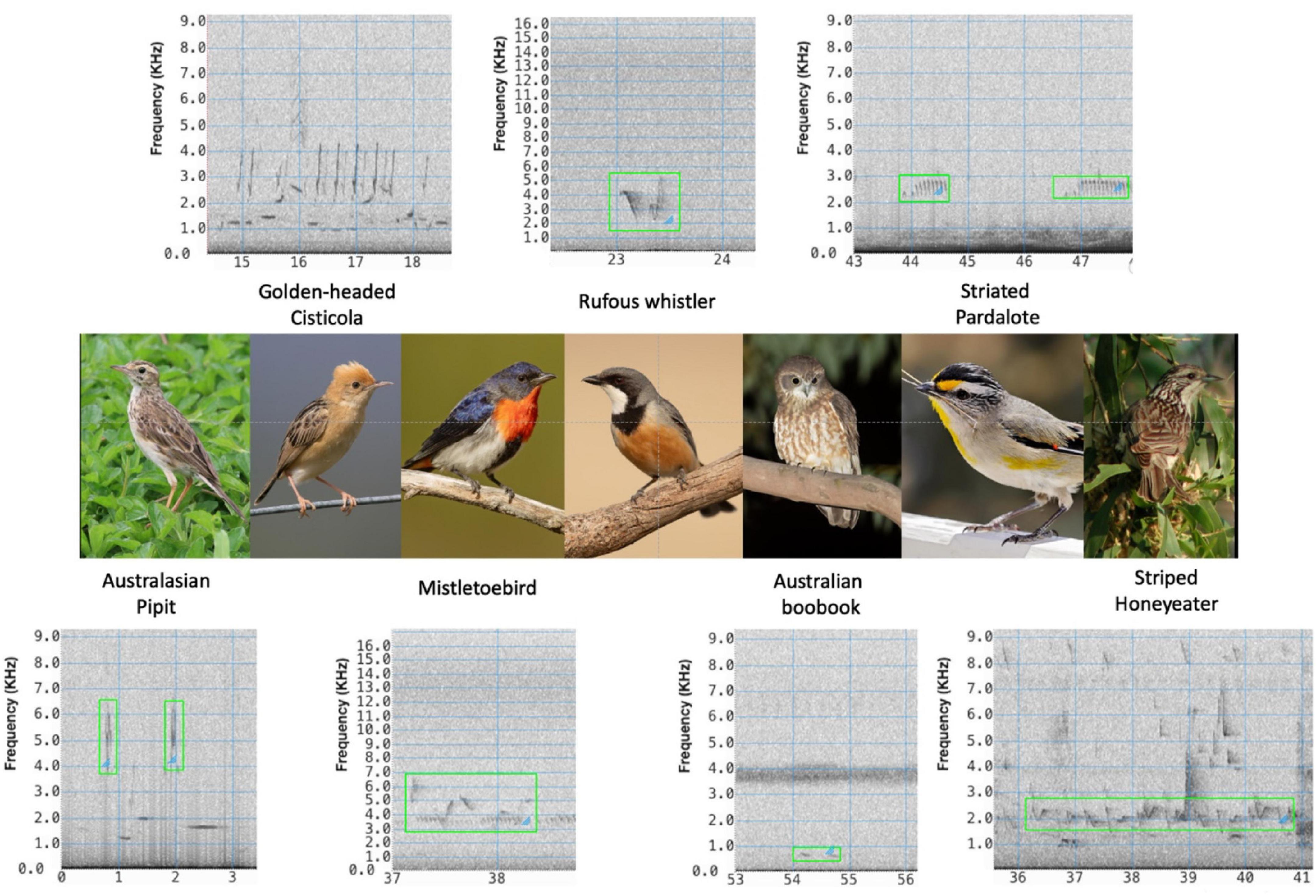
Figure 1. Target species and their vocalizations. Australiasian Pipit, photo credit: https://commons.wikimedia.org/wiki/User:Summerdrought; https://creative commons.org/licenses/by-sa/4.0/; Golden-headed Cisticola, Mistletoebird, Rufous Whistler, Australian Boobook, photo credit: https://commons.wikimedia.org/wiki/User:JJ_Harrison; https://creativecommons.org/licenses/by-sa/4.0/legalcode. Striated Pardalote, photo credit: https://en.wikipedia.org/wiki/User:Fir0002; https://creativecommons.org/licenses/by-nc/3.0/legalcode. Striped Honeyeater, photo credit: https://commons.wikimedia.org/wiki/User:Aviceda; https://creative commons.org/licenses/by-sa/3.0/legalcode.

These species were chosen based on several criteria. Firstly, they cover multiple functional groups of interest—insectivores, frugivores, nectarivores, and predators. Secondly, they are known to occur across multiple cotton growing regions within Australia (Smith et al., 2019). They are expected to be present in numbers where changes in the frequency of their presence will be detectable: i.e., not so common that they are always present no matter if the health of the ecosystem deteriorates or improves, but and not so rare that they never occur. Finally, they have reasonably distinguishable calls, compared to some other candidates.

The challenge was that we started with no labeled examples of these species in recordings from cotton regions. Using recordings from other regions we built a recognizer that was able to find enough of the target species that it could be used to optimize the process of manually labeling cotton recordings to build the training dataset. This process was iterated, with each iteration adding more examples from cotton regions.

Related Research

For the last decade or more, interest in using acoustics for ecological monitoring has been steadily increasing, bolstered by a drop in the price for recording hardware and storage (Roe et al., 2021) and more recently by advances in automated analysis (Xie et al., 2019). For a number of years, deep learning techniques have dominated these automated analysis approaches (Gupta et al., 2021). In the 2018 Bird Audio Detection challenge a competition for classifying 10-s audio clips as containing a bird or not, the highest performing entries were all convolutional neural networks, with the most accurate results achieved using a transfer learning setup, with both resnet50 and inception models (Lasseck, 2018).

Deep learning models, and machine learning models in general, are trained on one set of examples, and tested on a different set, referred to as the test set. Much published research uses datasets where the training data and test data are drawn from the same datasets (Narasimhan et al., 2017; Xu et al., 2020). While this is valuable and interesting for exploring different algorithms, in many real-world ecological applications the model will be deployed in new environments. Other research tests models on datasets not used in training (Stowell et al., 2019), which is a much more challenging test of generalizability of the models.

This paper describes challenges related to this ability for the model to generalize from one dataset to another. Most of the literature presents an academic exercise in increasing accuracy on an available test dataset. There is little research published on how to approach the situation where the species recognizer is to be deployed for a real-world ecological purpose but data from that deployment location does not exist.

The main approach we took is an active learning approach. Generally speaking, active learning involves the model making predictions on unlabeled examples, selecting the most informative of these for labeling based on a query strategy, querying an oracle for the label, and then updating its weights based on this new training example (Cohn et al., 1994; Wang et al., 2019). This technique has been proposed in a number of ecoacoustics studies: Kholghi et al. (2018) adopted this approach to speed up labeling audio for soundscape classification. Qian et al. (2017) assessed the performance of active learning for classifying a library of bird calls. These studies, however, are made on constrained artificial tasks, and tend to focus on the mathematics of the query strategy for selecting new samples.

This paper describes our experience in applying an active learning approach to developing species recognizers for our biodiversity monitoring project, using a mismatched initial labeled dataset. As well as describing the network architecture and active learning query strategy, we describe the progression of how the dataset grew, and how the accuracy metrics for each target species changed accordingly.

Materials and Methods

Dataset Building Through Verification of Results

Data Sources

Original Dataset

Ecosounds¹ is a website built using the QUT Ecoacoustics Workbench (Truskinger and Cottman-Fields, 2017) and serves as a repository for annotated ecological audio recordings. It contains several datasets for which we had permission to use, and which served as a starting point. These recordings were from a variety of locations in eastern Australia, but none of which were cotton regions. This dataset consisted of recordings with vocalizations annotated with time and frequency bounds of variable length. The numbers of examples for each species from this dataset is shown in Table 1.

TABLE 1

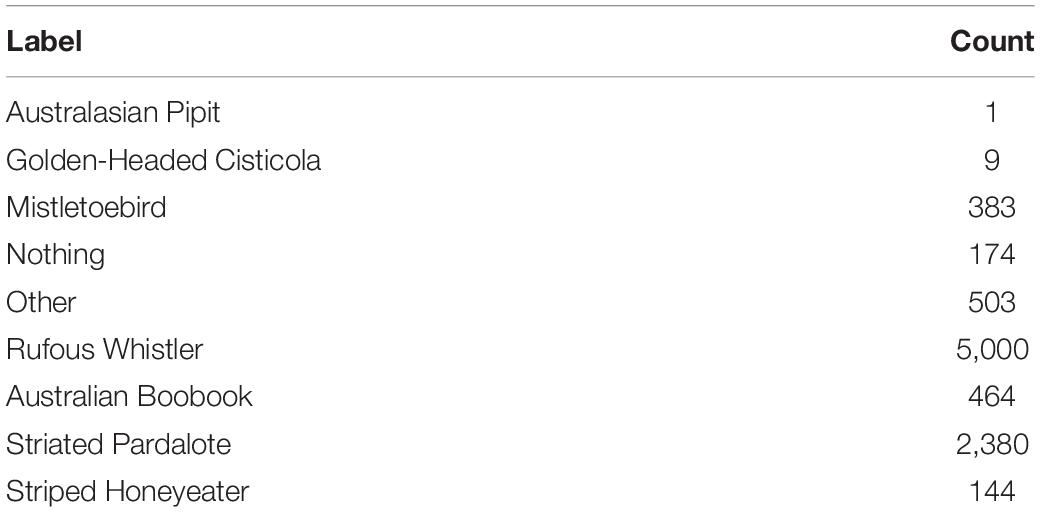
Table 1. Number of initial recordings from other regions.

In addition to examples of the target species, a varied selection of negative examples was also included in the training data. Examples from every non-target species available to us was included. The class containing non-target species events is referred to as “other.”

Cotton Recordings

We deployed Song Meter SM3 recorders (Wildlife Acoustics) on Australian cotton farms in the Narrabri region of northern New South Wales in early 2020, and the St George, Miles and Dalby regions of southern Queensland in late 2020 and early 2021, shown in Figure 2 and Table 2. The recorders were programmed to record for 2 h starting just before dawn and 1 h during dusk at 24 kHz and default gain settings. Ecosounds was used to store and later annotate these cotton recordings.

FIGURE 2

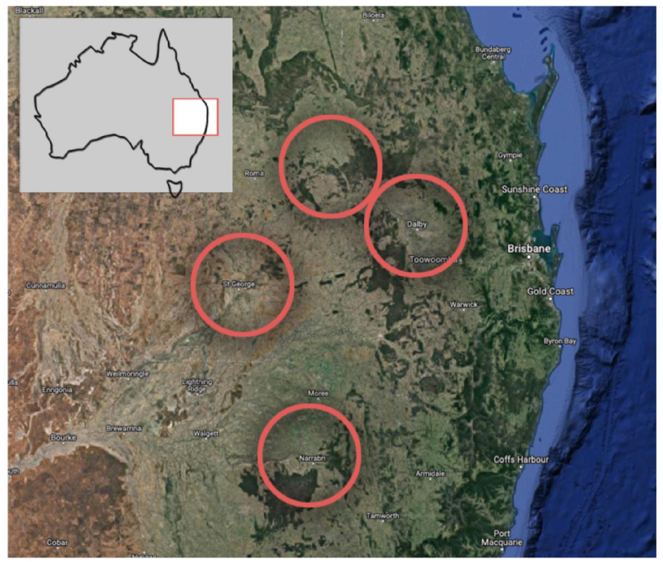
Figure 2. Cotton regions where recordings were taken. Imagery (C)2021 Landsat/Copernicus, Data SIO, NOAA, U.S. Navy, NGA, GEBCO, Imagery (C)2021 TerraMetrics, Map data (C)2021 Google.

TABLE 2

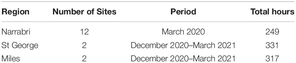
Table 2. Recording period for training data.

Convolutional Neural Network Verification Workflow

Figure 3 illustrates the workflow to build the dataset so that it contains examples from the cotton recordings.

FIGURE 3

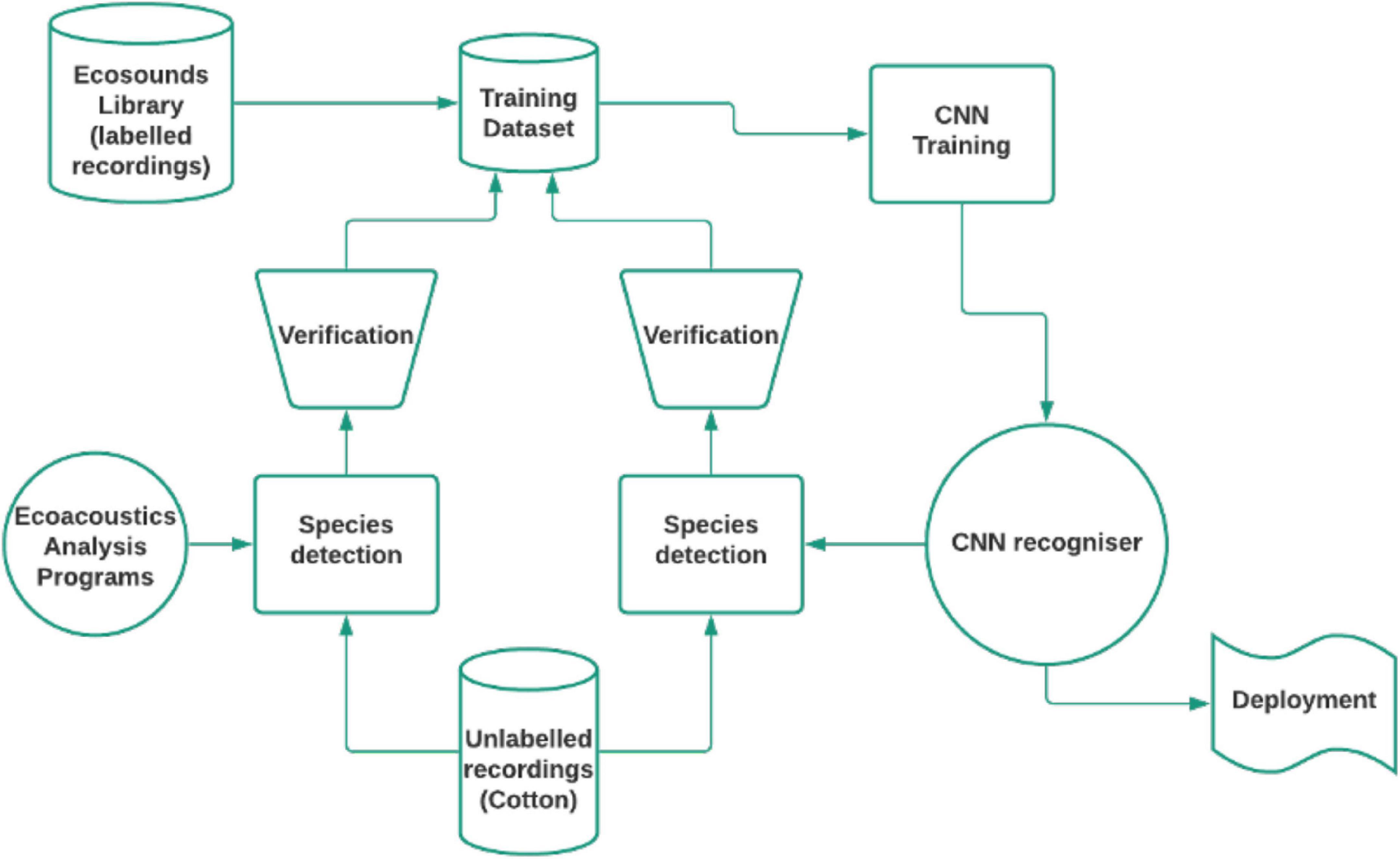
Figure 3. Iterative workflow for verifying classification results.

Initial Labeling of Cotton Recording

Two species were under-represented in the non-cotton dataset: Australasian Pipit and the Golden-headed Cisticola. Recognizers were built for these species, using the QUT Ecoacoustic Analysis Programs software (Towsey et al., 2020). These do not use learned features or machine learning but rather use human-designed features with thresholds manually set based on human knowledge about the call structure. The results of these recognizers were used to filter the cotton recordings. Combined with some random manual sampling, this provided sufficient examples to initiate training of the CNN, however, due to the high number of false positives and scarcity of the target species, it was a slow and inefficient exercise. A recognizer was also built for Australian Boobook as this was an easier task due to the simple call structure and quieter time (night) when they are active. Through this process, a variety of examples for the negative classes as well as a handful of examples for other target species were found. The numbers for each species are show in column T1 of Table 3.

TABLE 3

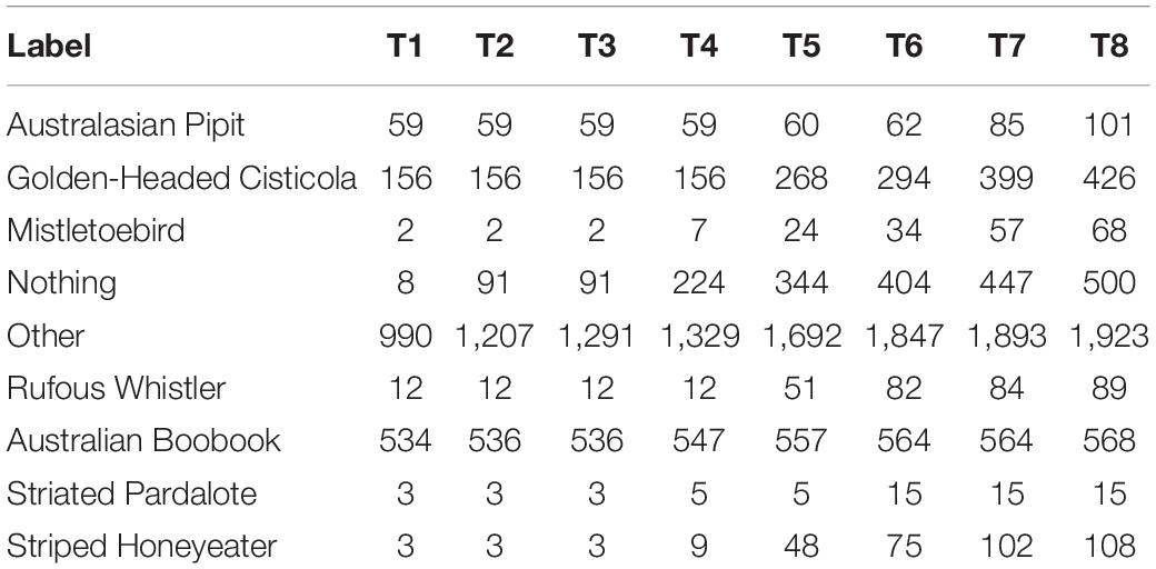
Table 3. Number of examples from cotton region recordings for each class at each iteration T1 to T8.

Training and Verification

Using a dataset comprised of both these initial cotton annotations and the non-cotton annotations, the CNN was trained. Then the following steps were performed repeatedly.

• The long unlabeled recordings were segmented into non-overlapping 4 s segments which were each then classified as belonging to one of the seven positive classes or on of the two negative classes. As well as the predicted class, the network also provides the probability for every class.

• These predictions and probabilities were then used to select the subset that was most likely to contain examples of the target species. Links to find these segments on ecosounds were generated.

• An expert avian ecologist then correctly annotated the selected segments.

• The dataset was recreated from all available annotations, including these new additions.

This kind of iterative process is known as active learning. New examples are added to the training set by selecting them based on the estimated new information they will add to the classifier.

Query Strategy for Selection of Segments for Verification

For the initial iterations, there were low numbers of detections for the positive classes. For many of the classes none of the segments were classified as that class. As these were unlabeled segments, it was not possible to know whether this was because there were few individuals of those species present in those recordings or the recall for those species was very low.

A protocol for selection of the subset for human verification was designed with the goals of (a) increasing the number of examples of each of the target species (b) correctly labeling the segments that the classifier was least sure about.

Firstly, for each species we included the 20 examples with the highest probability for that class. In cases where there were fewer than 20 segments classified as that class, we still selected the top 20 examples using the probabilities output by the CNN. That is, a particular segment might be the highest scoring for one species even if that probability is lower than the probability for another species. An example with a very high probability that is verified to be correct may only marginally improve the recognizer performance. This is because, for the particular variations of the vocalization that is added to the training set, the network is already performing well. However, if it turns out that these high probability predictions were incorrect, then it is very valuable to include them as training examples to rectify these mistakes in subsequent iterations. Furthermore, an example that the recognizer correctly identifies is often the case that other examples are present nearby in the recording that may not have been detected. These can be easily manually scanned for and added by navigating in the Ecosounds interface.

Secondly, for each species, we included for verification the 10 examples that were classified as that class (or fewer if there were fewer than 10 detections) but had the lowest probability of belonging to that class—those that the CNN was least sure about. These are likely to contain interesting and unique confusing sounds, and are therefore valuable to include in the dataset.

Thirdly, for each species we included a random selection of 10 segments that were classified as belonging to that class (or fewer if there were fewer than 10 detections). This can be used to get an idea of the precision for each class.

For the “other” and “nothing” classes, we did the same, but with only five examples between them. The reason for this lower number, is that examples of these classes are very easy to find and are likely to be included through false positive detections of the bird species.

This resulted in a maximum of 300, 4-s segments to verify on each iteration. However, the actual number may be fewer, as the same segments can be included in more than one selection, especially where there were few or no detections for some species.

Incorporation of Verified Samples Into the Dataset

For each of these, links were generated to view and listen to the segments on the Ecosounds website, with some padding to give more context. These verified segments now have annotations that are then incorporated into the training/testing.

To ensure that the accuracies for the model trained on different stages of the dataset were comparable with each other, the model is retrained from scratch (i.e., transfer learning from the initial weights provided by the model, described in the next section), rather than fine tuning the previously trained model.

We repeated this process a total of eight times. Table 3 shows the number of examples from cotton regions after each iteration.

Convolutional Neural Network Architecture and Data Preprocessing

Convolutional Neural Network Architecture

The CNN architecture that was chosen is Resnet34 (He et al., 2015). It is a deep convolutional neural network designed for image classification, but which has been shown to perform well when trained on ecological audio (Lasseck, 2018). It is a model that has been tested in many applications and the model parameters pre-trained on a large image dataset are available to allow transfer learning. The input to this architecture is a square image of size 224 × 224 pixels. The network was implemented and trained using the FastAI python library (Howard and Gugger, 2018), built on Pytorch.

The output of the final fully connected layer is passed through a softmax function to give a probability for each class. In addition to a class for each of the seven target species, there is one for events that were not vocalizations from the target species labeled as “other,” and one for segments that only contain background noise, labeled as “nothing.” Collectively these two classes will be referred to as “negative examples.” The decision to separate the negative class into “other” and “nothing” was made due to the likely ease of determining the difference of discriminating between these two and the potential usefulness of being able to filter silent segments for applications like random sampling in the future.

The CNN does not localize the vocalization to a region within the input segment, but simply selects which of the classes the segment belongs to. We chose to use a single class architecture, meaning that it assumes that only one of the target species will be present, with the probabilities for all the classes adding to one. While this assumption may not necessarily always be true, we did not come across any examples in cotton recordings where this was the case. In the event that it does occur the pipeline for extracting training examples from our library is set such that it would include separate overlapping examples for the two species. While this would necessarily cause the accuracy on one of the two species to suffer slightly, it happened so infrequently that it was deemed to be worth the benefit of the simplified architecture as well as the dataset curation that a single class classifier brings.

Audio Preprocessing

The annotations from which the training set was generated were of variable length, due to the variable length nature of the vocalizations. The CNN network requires a fixed size input. While this could be achieved through simply squashing the image down, as is common in standard image recognition, the nature of spectrograms means this is unlikely to be appropriate. Instead, a fixed duration segment of the variable length segment was cropped at random from the longer variable length segment as the input to the network. A different random crop was taken each time the image was fed into the network. To allow for this random cropping, for each annotation, a 1 s padding was added before and after the full second marks that enclose the annotation, or if the annotation was less than 4 s, the annotation was centered in a 6 s clip with the boundaries on the nearest whole second. For these short events, when cropped randomly, the resulting 4 s segment contains the entire vocalization. This is illustrated in Figure 4.

FIGURE 4

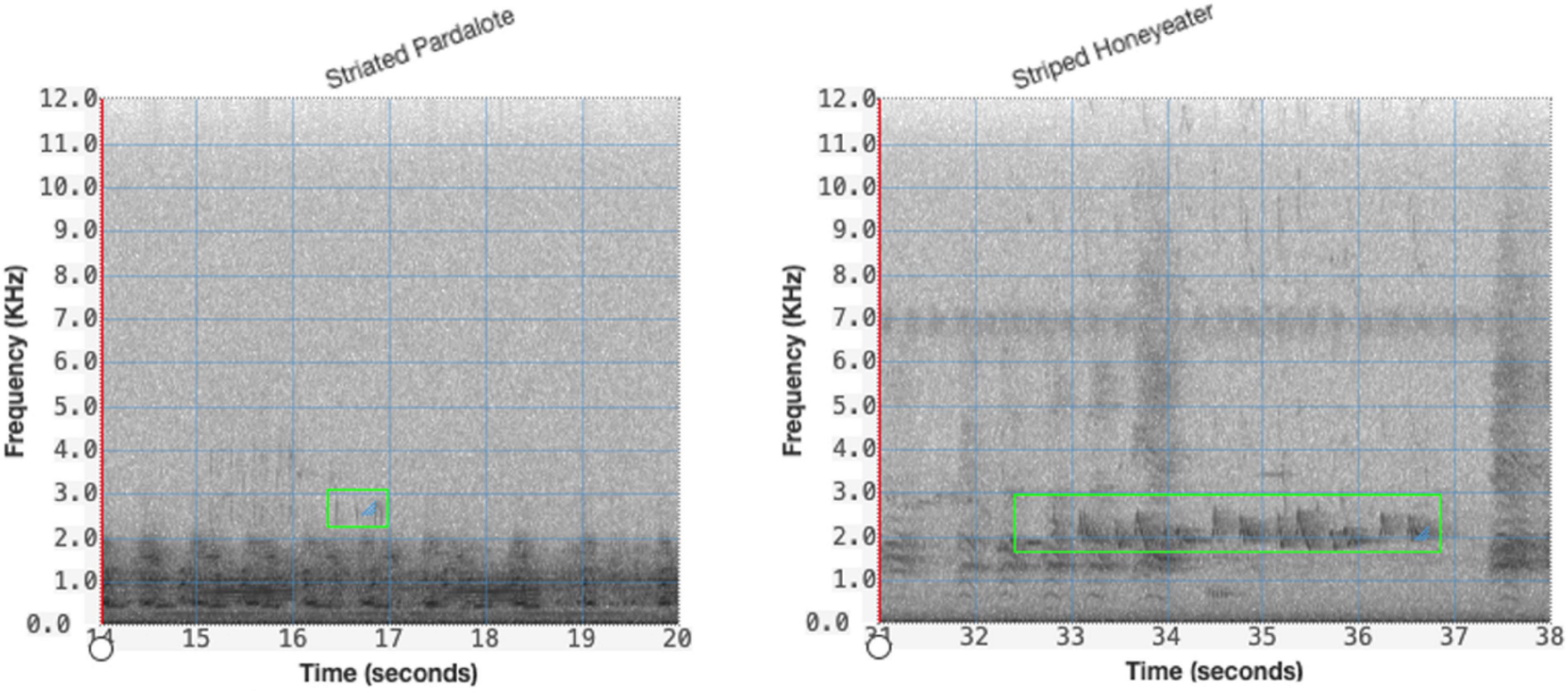
Figure 4. Segmentation of variable length audio, for both short (left) and long (right) annotations showing green bounding box of the time and frequency limits of the annotation.

The call library contains recordings at a variety of different sample rates. For the resulting spectrogram images to be comparable with each other, the inputs to the CNN should all be at the same sample rate. For this reason, all recordings were resampled to 16,000 Hz. Below are some considerations in choosing the frequency to resample to.

Because the number of rows of the spectrogram is fixed, lowering the top frequency gives a higher frequency resolution. However, it may not be desirable to down-sample too far. By including at least some of the frequency band above the top frequency of the target calls, more information is available to the CNN. For example, it may be that some acoustic event resembles the target species vocalization within the low frequency band, but also extends into the high frequencies, and this is the information that can be used to successfully discriminate.

Up-sampling is likely to be detrimental, and so the common frequency to resample to must be equal to or lower than the lowest frequency of the testing/training sets. Up-sampling will introduce artificial blank space at the top of the spectrogram, which could bias the network if certain classes are more likely to occur in those recordings. That is, the network might make an association between up-sampled audio and a given class.

Spectrogram Generation

For each variable length audio segment, a mel-scale spectrogram was generated. With 16 kHz audio, a short time Fourier transform (STFT) hop length is 286 samples to fit the desired 224-pixel width of 4 s of spectrogram. We found this works well with a window size of 512 samples with overlap of 226 samples (44%). A high pass of 100 Hz was applied to remove very low background noise. The python librosa package was used to produce a mel-scale spectrogram. The mel-scale increases the frequency resolution for low frequencies and reduces it for high frequencies.

The amplitude was converted to a log scale, a common practice for audio processing, and more closely represents the way that the ear processes sound. That is, a certain difference in amplitude between two low amplitude sounds will be more noticeable than the difference in amplitude between two high amplitude sounds. These log amplitude values were then normalized between 0 and 255 to produce the pixel color. Normalizing over very short duration audio can have drawbacks. If the segment is very quiet or contains only background noise, this background noise is unnaturally amplified. However, this does not seem to cause the performance of the network to suffer and is a simple way to scale to pixel values.

Resnet was originally designed for red-green-blue (RGB) color images, with the input a 224 × 224 × 3 tensor. The spectrogram is a two-dimensional grid of log amplitude values. These values of the pixels can be mapped to a three-dimensional array using a number of different color mapping schemes, for example red for high values and blue for low values. This kind of color mapping is often used when visualizing spectrograms for human viewers as it can be aesthetic, since loud events stand out from the background as a different color. We opted for a simpler grayscale mapping where the spectrogram is duplicated to each of the three color channels, as it is easier to implement, and there does not appear to be any evidence in the literature that grayscale is worse. The computational overhead for redundant layers on the input is negligible.

Spectrograms were pre-generated rather than generated on the fly as part of the pipeline. This accelerates the training process as spectrograms can be generated once rather than every epoch.

Data Augmentation

Training was performed on spectrograms of 4-s clips. Four seconds was chosen for a number of reasons. Vocalizations of the target species can be longer than 4 s, and the audio segment needs to be long enough that it captures enough of the vocalization to distinguish the class. However, it cannot be too long as this will increase the likelihood that other sounds will be included, and very short vocalizations would comprise a very small proportion of the overall size of the spectrogram image. The duration also needs to be reasonable to fit a square spectrogram image.

The training examples were of variable length depending on the duration of the example vocalization. On each epoch of training, a random 4 s segment was taken from the variable length segment. This trains the network to discriminate calls no matter which point of time they appear in the 4 s segment, that is the recognizer is time invariant.

Training examples were also blended with negative examples taken from cotton regions from the training set. Negative examples were selected, multiplied by between 0.1 and 0.3 randomly then added to the augmented training example before normalization, which has the effect of audio-mixing on the spectrogram images. This effectively synthesizes new training examples with not only more variety of background sounds, but background sounds that appear in the soundscape where the recognizer will be eventually deployed.

All data augmentation was performed on the fly for each batch of forward propagation on the training set, and the number of training examples mentioned in this paper does not include the contribution of augmentation.

Training

Examples were randomly allocated as either training (85%) or testing (15%). This was done deterministically for each file by taking a cryptographic hash of the id for the annotation mod 100 and splitting it according to the resulting value. This has the advantage of easily ensuring that a particular example would always belong to the same part of the split, which potentially allows for finetuning of the model produced by the previous iteration of the verification loop (although we chose not to do this so that the results could be compared between each iteration) without cross contamination between training and test sets. The drawback is that for classes with very few examples, the proportion of training examples can end up being greater or less than 85%. Often in machine learning there is a third dataset split, the validation set, which is used to calculate metrics to inform hyperparameter tuning during the course of training, however, this was not applicable to our design.

To prevent the massive class imbalance in the dataset from biasing the CNN, care was taken in training so that on each epoch the network used the same number of examples from each class. This was achieved by repeating examples from classes that had few examples. Thus, the only class that had its examples fed into the network exactly once per epoch was the class with the most examples (Rufous Whistler). Training continued for four epochs, as this was when the test set error rate stopped showing improvement.

Results

After each iteration of training, metrics were calculated on the test set. For each class the precision (the fraction items predicted to belong to the class which were correct), and recall (the fraction of items that belong to the class which were predicted as belonging to that class) were calculated, as well as the F1 score, the harmonic mean of the precision and recall. We also determined the overall accuracy, which is the fraction of items that were predicted correctly, however, since our dataset was so unbalanced, this may give an over-optimistic picture, as classes that contributed most to the accuracy because they had a lot of examples also tended to have higher precision and recall. We prefer to summarize by averaging precision, recall and F1 across the classes with each class weighted equally. This macro average of F1 score was deemed the most important metric for the overall performance of the recognizer.

Table 4 lists all the metrics for the recognizer after the first and last iteration of training, as well as the middle iteration to give a sense of the progress. The macro average F1 score increased from 0.45 to 0.74 between the first iteration (T1) and the final iteration (T8). Also included are the confusion matrix for T1 and T8 in Figure 5.

TABLE 4

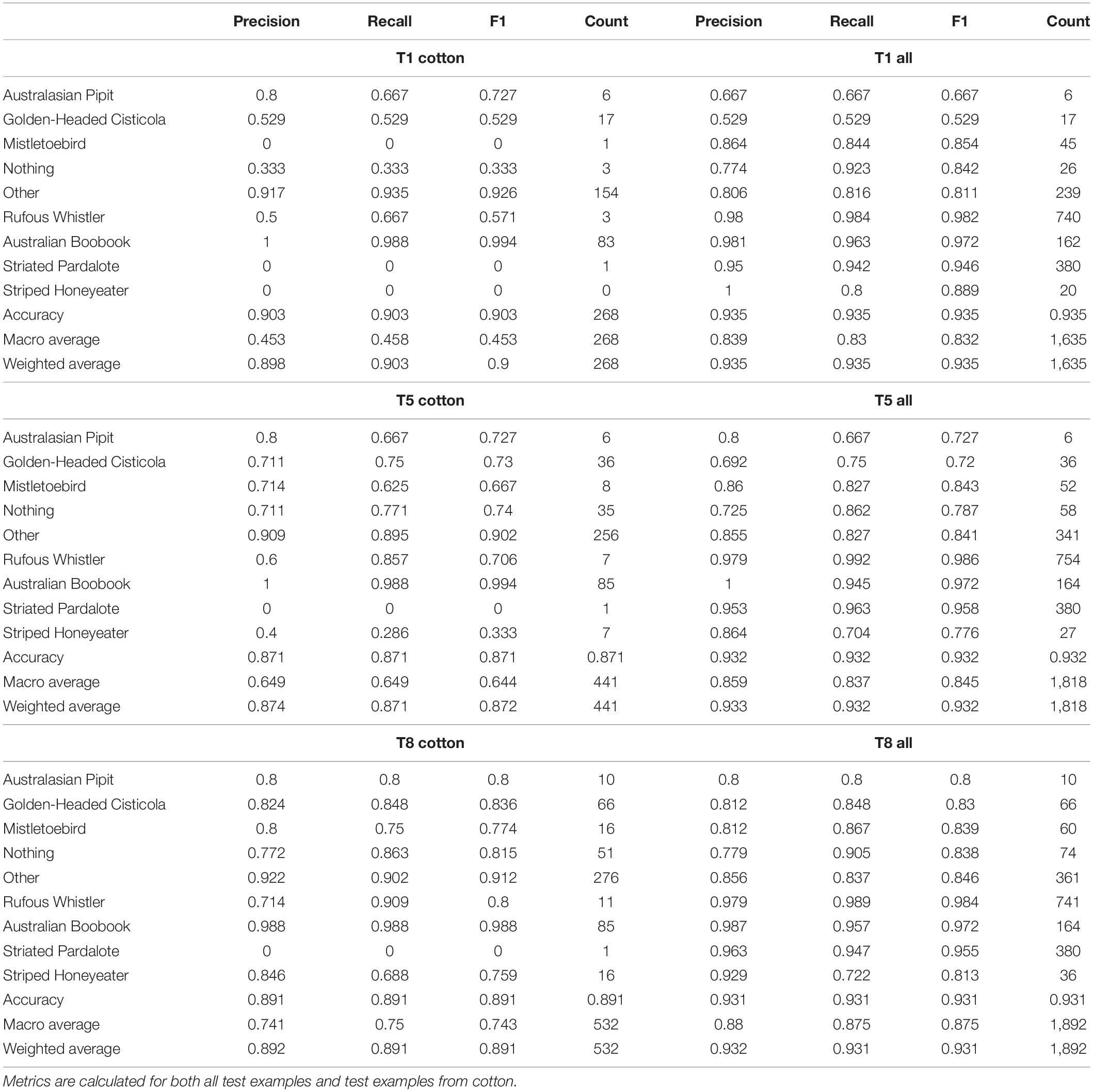
Table 4. Metrics for classification on test set for iteration 1, 5, and 8.

FIGURE 5

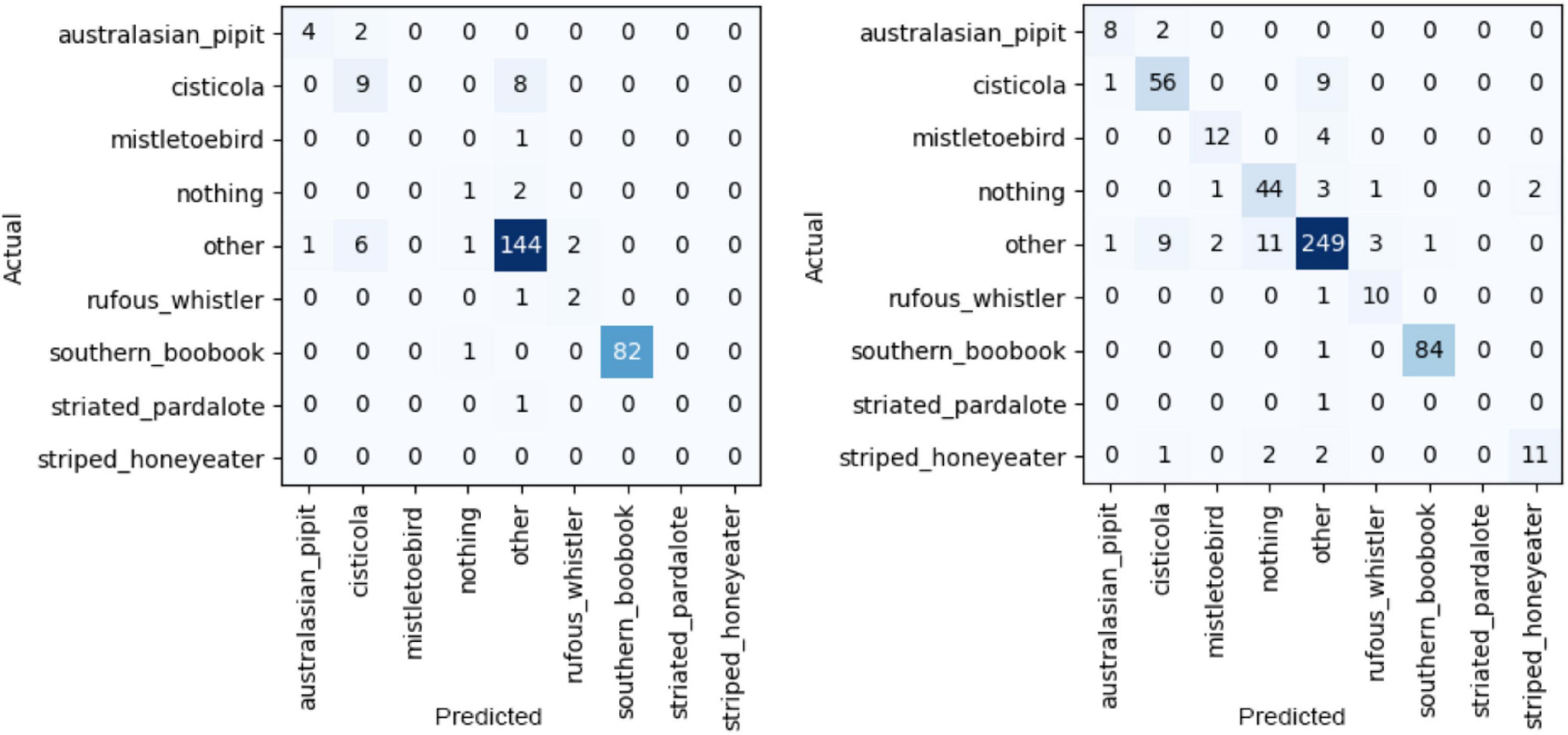
Figure 5. Confusion matrix for T1 (left) and T8 (right).

The results differed for each of the classes, depending on the ease of discriminating species calls, the number of examples in both cotton and non-cotton, and the abundance of the species in the unlabeled cotton recordings used to build the dataset.

The Rufous Whistler was an interesting example. Initially we had thousands of examples from non-cotton regions, but only 12 from cotton regions, three of which were included at random in the test set. The initial precision and recall over the entire test set was very high (F1 score of 0.98), however this did not generalize to cotton with 0.5 precision and 0.67 recall, although with such a small number the recall especially may be heavily influenced by random variation. For the 5th iteration (T5) we had added 39 new examples and the precision and recall increased to 0.6 and 0.86, respectively. Finally, for the 8th iteration there were a total of 89 examples, with the precision and recall increasing to 0.71 and 0.91, respectively. This improvement is interesting since, although the number of examples of Rufous Whistler in cotton increased more than sevenfold, this still comprised less than 2% of the examples.

The Australian Boobook and the “other” class showed no improvement, as they were already performing quite well with the initial cotton examples that were added through the verification of non-machine-learning Ecoacoustics Analysis Programs detections. The Australian Boobook was the least challenging of the seven target species because it is active at night when there are fewer confusing sounds. The recall of the “other” class lowered slightly as the dataset was built. This might be because the sheer variety of events that belong to the “other” means that, although we were adding misclassified confusing events into the training set for “other,” we were also adding confusing events to the test set that were not necessarily similar to those added training examples. Regardless, this slight drop in recall for the negative classes has no impact on the usefulness of the model as a species detector.

Some species were not found in great numbers using the verification loop workflow. The Australasian Pipit initially had 59 examples from cotton, which was increased to 101. The reported recall in cotton for the Australasian Pipit was initially 0.68, meaning that it should have been able to detect this species in the unlabeled recordings. It is possible that Australasian Pipits were not present or not particularly active during the time period during which the recordings were made. This species was largely absent from the non-cotton recordings, however, there were enough found through the early laborious efforts to create some initial examples.

The Striated Pardalote initially only had three examples from cotton region recordings, with over 2,000 from non-cotton recordings. The is eventually increased to 15 examples, however due to the way that training, and test data was split, only one example was included in the test set. The recall on non-cotton recordings was quite high at 0.93, and therefore we would have expected to find more examples in cotton if they were present.

The Striped Honeyeater was one of the species with the best improvement. It initially had only three examples from cotton recordings, none of which ended up in the test data, and so metrics could not be calculated. At T5 the number of examples had increased to 48, and the F1 score from the model trained on this was 0.3. By T8 the number of examples had grown to 108 and the F1 score increased to 0.76.

The overall macro average F1 of the test set of all recordings also increased from 0.83 to 0.88. This was initially surprising, since the overall number of new examples from cotton recordings added was only a fraction of the total recordings. However, for some classes, namely Australasian Pipit, other, nothing, and Striped Honeyeater, the proportion of new examples added between T1 and T8 was high.

It can be seen that the first few iterations were relatively unsuccessful in finding new examples across many of the species, and then the rate of finding new examples started to accelerate. One explanation for this might be that early on there were many incorrect detections of target species that were labeled as “other” on verification. It wasn’t until the after this initial addition to the training set of confusing sounds present only in the deployment location that the model was able to reduce false positive rate enough for target species to begin to be added.

Discussion

Example of Data Mismatch

A potential cause for mismatch is a systematic bias in the labeled recordings. For example, our labeled Australian Boobook recordings, which were made at night, were often accompanied by cicadas stridulating. Our negative set of recordings of class “other” was designed to include a wide variety of calls by sampling from the full range of annotations. However, this did not happen to contain many annotations of cicadas. This led to the CNN learning to associate the presence of cicadas with Australian Boobooks and therefore produced many false positive Australian Boobook detections where cicadas were present. In this example, the one iteration of verifications remedied this; these false positives were added to the training set and the precision for Australian Boobooks increased.

Bias Introduced Through Feedback

A limitation of using results from a classifier to find more training examples is that it may be missing a certain variety of call type that were never included and therefore it continues to miss. While we can estimate the proportion of detections of each class that were correct (precision), which gives the false positive rate, it is not possible to measure the proportion of each class in unlabeled recordings that were found (recall), as only a small fraction of the analyzed duration is verified, meaning we can’t know the false negative rate. We tried to address this as best as we could by doing some random sampling of segments in close temporal proximity to any true positive detection. This is because it is likely that individuals or members of the group will call repeatedly, and this approach had some success on occasion. However, the expertise of the ecologist doing the verifications is important here, as their knowledge of the habits of the different species at different seasons, times of day and vegetation types informed their decision to dedicate time to this search.

Acceptable F1 Scores for Drawing Conclusions

The main purpose of this classifier is to detect differences in species richness among the target species over long periods of time, drawing on the aggregations of many individual predictions of 4-s segments. It is possible to compare the presence of a particular species between two sets of many recordings even with a number of errors, as this process of aggregation removes the impact of the individual errors. In theory, as long as the errors are made in a consistent way across the two sets of recordings being compared, any F1 score above that of random guessing (0.11 for a nine-class classifier) could still be useful if aggregated across enough data. Of course, in reality, the errors will not necessarily be random or consistent. For example, there may be a sound source that causes confusion present in one of the sets of recordings and not the other. Most of our target species ended with F1 scores around 0.8–0.9, which should be enough to compare sets of recordings on aggregate, even with the potential of these confusing sounds not being spread evenly across the recordings.

Conclusion

Through an iterative process of training, classifying unlabeled recordings, verifying and retraining, we were able to build a dataset for the cotton regions of eastern Australia that can be used to train a convolutional neural network to achieve a macro average F1 score across seven target species of birds plus two negative classes of 0.74%. This F1 score would likely continue to improve with further iterations. In the future, this ecoacoustic analytical approach will be deployed with the aim of monitoring changes in the mean proportion of functional guilds of birds in response to on-farm vegetation management in cotton growing regions of Australia, providing valuable information to assist the cotton industry in preserving biodiversity.

Data Availability Statement

Data for this research was provided by several sources and not all of them have given permission for the data to be made publicly available. Requests to access the datasets should be directed to the corresponding author (cGhpbGlwLmVpY2hpbnNraUBxdXQuZWR1LmF1).

Author Contributions

PE: coding and running the CNN and other software scripts required for this research and writing the manuscript. CA: creation of the dataset by labeling audio examples and fieldwork making recordings. PR: advising on data collection, labeling and curation strategies, and planning the manuscript structure. SP: advising on data collection, labeling and curation strategies, planning the manuscript structure, and leading the project. SF: designing the study, fieldwork making recordings, planning the manuscript structure, and editing. All authors contributed to the article and approved the submitted version.

Funding

Funding for this research was provided by the Cotton Research and Development Corporation (CRDC, Grant No. NLP1901).

Conflict of Interest

The authors declare that the research was conducted in the absence of any commercial or financial relationships that could be construed as a potential conflict of interest.

Publisher’s Note

All claims expressed in this article are solely those of the authors and do not necessarily represent those of their affiliated organizations, or those of the publisher, the editors and the reviewers. Any product that may be evaluated in this article, or claim that may be made by its manufacturer, is not guaranteed or endorsed by the publisher.

Acknowledgments

We thank Yvonne Phillips, Brendan Doohan, and David Tucker for allowing us to use their labeled recordings. We also thank the following cotton growers—Hamish McIntyre, Tamara Uebergang, and Mark Harms—for generously hosting acoustic sensors on their cotton farms for 5 months. We acknowledge the conceptual and initial research contribution of Erin Peterson on this research project. We also acknowledge the Cotton Research and Development Corporation for funding this research.

Footnotes

1. ^ www.ecosounds.org

References

Acevedo, M. A., and Villanueva-Rivera, L. J. (2006). From the field: using automated digital recording systems as effective tools for the monitoring of birds and amphibians. Wildlife Soc. Bull. 34, 211–214.

Google Scholar

Both, C., Van Turnhout, C. A. M., Bijlsma, R. G., Siepel, H., Van Strien, A. J., and Foppen, R. P. B. (2010). Avian population consequences of climate change are most severe for long-distance migrants in seasonal habitats. Proc. R. Soc. B Biol. Sci. 277, 1259–1266. doi: 10.1098/rspb.2009.1525

PubMed Abstract | CrossRef Full Text | Google Scholar

Cohn, D., Atlas, L., and Ladner, R. (1994). Improving generalization with active learning. Mach. Learn. 15, 201–221.

Google Scholar

Dockès, J., Varoquaux, G., and Poline, J.-B. (2021). Preventing dataset shift from breaking machine-learning biomarkers. Gigascience 10:giab055. doi: 10.1093/gigascience/giab055

PubMed Abstract | CrossRef Full Text | Google Scholar

Garcia, K., Olimpi, E. M., Karp, D. S., and Gonthier, D. J. (2020). The good, the bad, and the risky: can birds be incorporated as biological control agents into integrated pest management programs? J. Integ. Pest Manag. 11:11. doi: 10.1093/jipm/pmaa009

CrossRef Full Text | Google Scholar

Gupta, G., Kshirsagar, M., Zhong, M., Gholami, S., and Ferres, J. L. (2021). Comparing recurrent convolutional neural networks for large scale bird species classification. Sci. Rep. 11:17085. doi: 10.1038/s41598-021-96446-w

PubMed Abstract | CrossRef Full Text | Google Scholar

He, K., Zhang, X., Ren, S., and Sun, J. (2015). Deep residual learning for image recognition. arXiv [cs.CV] [Preprint].

Google Scholar

Howard, J., and Gugger, S. (2018). Fastai: a layered api for deep learning arXiv [Preprint]. doi: 10.3390/info11020108

CrossRef Full Text | Google Scholar

Kholghi, M., Phillips, Y., Towsey, M., Sitbon, L., and Roe, P. (2018). Active learning for classifying long-duration audio recordings of the environment. Methods Ecol. Evol. 9, 1948–1958. doi: 10.1111/2041-210X.13042

CrossRef Full Text | Google Scholar

Kouw, W. M., and Loog, M. (2021). A review of domain adaptation without target labels. IEEE Trans. Pattern Anal. Mach. Intell. 43, 766–785. doi: 10.1109/TPAMI.2019.2945942

PubMed Abstract | CrossRef Full Text | Google Scholar

Kumar, A., Prakash, G., and Kumar, G. (2021). Does environmentally responsible purchase intention matter for consumers? A predictive sustainable model developed through an empirical study. J. Retail. Consum. Serv. 58:102270. doi: 10.1016/j.jretconser.2020.102270

CrossRef Full Text | Google Scholar

Lasseck, M. (2018). “Acoustic bird detection with deep convolutional neural networks,” in Detection and Classification of Acoustic Scenes and Events, eds D. Stowell D. Giannoulis E. Benetos M. Lagrange and M. D. Plumble (Piscataway, NJ: IEEE).

Google Scholar

Leseberg, N. P., Venables, W. N., Murphy, S. A., and Watson, J. E. M. (2020). Using intrinsic and contextual information associated with automated signal detections to improve call recognizer performance: a case study using the cryptic and critically endangered Night Parrot Pezoporus occidentalis. Methods Ecol. Evol. 11, 1520–1530. doi: 10.1111/2041-210X.13475

CrossRef Full Text | Google Scholar

Narasimhan, R., Fern, X. Z., and Raich, R. (2017). “Simultaneous segmentation and classification of bird song using CNN,” in Proceedings of the 2017 IEEE International Conference on Acoustics, Speech and Signal Processing (ICASSP), (Piscataway, NJ: IEEE), 146–150.

Google Scholar

Newell, F. L., Sheehan, J., Wood, P. B., Rodewald, A. D., Buehler, D. A., Keyser, P. D., et al. (2013). Comparison of point counts and territory mapping for detecting effects of forest management on songbirds. J. Field Ornithol. 84, 270–286.

Google Scholar

Qian, K., Zhang, Z., Baird, A., and Schuller, B. (2017). Active learning for bird sound classification via a kernel-based extreme learning machine. J. Acoust. Soc. Am. 142, 1796–1804. doi: 10.1121/1.5004570

PubMed Abstract | CrossRef Full Text | Google Scholar

Roe, P., Eichinski, P., Fuller, R. A., McDonald, P. G., Schwarzkopf, L., Towsey, M., et al. (2021). The Australian acoustic observatory. Methods Ecol. Evol. 12, 1802–1808.

Google Scholar

Smith, R., Reid, J., Scott-Morales, L., Green, S., and Reid, N. (2019). A baseline survey of birds in native vegetation on cotton farms in inland eastern Australia. Wildlife Res. 46:313.

Google Scholar

Stacke, K., Eilertsen, G., Unger, J., and Lundström, C. (2021). Measuring domain shift for deep learning in histopathology. IEEE J. Biomed. Health Informatics 25, 325–336. doi: 10.1109/JBHI.2020.3032060

PubMed Abstract | CrossRef Full Text | Google Scholar

Stowell, D., Wood, M. D., Pamuła, H., Stylianou, Y., and Glotin, H. (2019). Automatic acoustic detection of birds through deep learning: the first bird audio detection challenge. Methods Ecol. Evol. 10, 368–380. doi: 10.1111/2041-210x.13103

CrossRef Full Text | Google Scholar

Teixeira, D., Hill, R., Barth, M., Maron, M., and van Rensburg, B. J. (2021). Vocal signals of ontogeny and fledging in nestling black-cockatoos: implications for monitoring. Bioacoustics 1–18. doi: 10.1080/09524622.2021.1941257

CrossRef Full Text | Google Scholar

Towsey, M., Truskinger, A., Cottman-Fields, M., and Roe, P. (eds) (2020). “Ecoacoustics audio analysis software,” in QutEcoacoustics/Audio-Analysis: Ecoacoustics Audio Analysis Software V20.11.2.0. (Genève: Zenodo). doi: 10.12688/f1000research.26369.1

PubMed Abstract | CrossRef Full Text | Google Scholar

Truskinger, A., and Cottman-Fields, M. (2017). Acoustic Workbench. Brisbane, Qld: QUT.

Google Scholar

Wang, Y., Mendez, A. E. M., Cartwright, M., and Bello, J. P. (2019). “Active learning for efficient audio annotation and classification with a large amount of unlabeled data,” in Proceeding of the ICASSP 2019-2019 IEEE International Conference On Acoustics, Speech And Signal Processing (ICASSP), (Piscataway, NJ: IEEE), 880–884.

Google Scholar

Wimmer, J., Towsey, M., Planitz, B., Williamson, I., and Roe, P. (2013). Analysing environmental acoustic data through collaboration and automation. Future Gener. Comput. Syst. 29, 560–568. doi: 10.1016/j.future.2012.03.004

CrossRef Full Text | Google Scholar

Xie, J., Hu, K., Zhu, M., Yu, J., and Zhu, Q. (2019). Investigation of different CNN-based models for improved bird sound classification. IEEE Access 7, 175353–175361.

Google Scholar

Xu, W., Zhang, X., Yao, L., Xue, W., and Wei, B. (2020). A multi-view CNN-based acoustic classification system for automatic animal species identification. Ad Hoc Netw. 102:102115.

Google Scholar