An Individual-Based Model of the Red Alga Agarophyton chilense Unravels the Complex Demography of Its Intertidal Stands

Algal demographic models have been developed mainly to study their life cycle evolution or optimize their commercial exploitation. Most commonly, structured-aggregated population models simulate the main life cycle stages considering their fertility, growth and survival. Their coarse resolution results in weak predictive abilities since neglected details may still impact the whole. In our case, we need a model of Agarophyton chilense natural intertidal populations that unravels the complex demography of isomorphic biphasic life cycles and be further used for: (i) introduction of genetics, aimed at studying the evolutionary stability of life cycles, (ii) optimizing commercial exploitation, and (iii) adaptation for other species. Long-term monitoring yield 6,066 individual observations and 40 population observations. For a holistic perspective, we developed an Individual-Based Model (IBM) considering ploidy stage, sex stage, holdfast age and survival, frond size, growth and breakage, fecundity, spore survival, stand biomass, location and season. The IBM was calibrated and validated comparing observed and estimated sizes and abundances of gametophyte males, gametophyte females and tetrasporophytes, stand biomass, haploid:dipoid ratio (known as H:D or G:T), fecundity and recruitment. The IBM replicated well the respective individual and population properties, and processes such as winter competition for light, self-thinning, summer stress from desiccation, frond breakage and re-growth, and different niche occupation by haploids and diploids. Its success depended on simulating with precision details such as the holdfasts’ dynamics. Because “details” often occur for a reduced number of individuals, inferring about them required going beyond statistically significant evidences and integrating these with parameter calibration aimed at maximized model fit. On average, the population was haploid-dominated (H:D > 1). In locations stressed by desiccation, the population was slightly biased toward the diploids and younger individuals due to the superior germination and survival of the diploid sporelings. In permanently submerged rock pools the population was biased toward the haploids and older individuals due to the superior growth and survival of the haploid adults. The IBM application demonstrated that conditional differentiation among ploidy stages was responsible for their differential niche occupation, which, in its turn, has been argued as the driver of the evolutionary stability of isomorphic biphasic life cycles.

Introduction

Seaweeds are the most efficient primary producers on the planet (Creed et al., 2019). In coastal waters, they often sustain the food web (Kang et al., 2008; Cordone et al., 2018; Momo et al., 2020), structure the community (Arkema et al., 2009; Momo et al., 2020) and are of commercial interest for mankind (Bustamante and Castilla, 1990; Guillemin et al., 2008; Lawton et al., 2013; Veeragurunathan et al., 2015; Mantri et al., 2020). Some algal species turned invasive, disrupting the functioning and balance of native communities (Staehr et al., 2000; Yamasaki et al., 2014; Davoult et al., 2017). Whatever the objective, the management of algal populations requires forecasting their evolution from current state and response to stimulus, either environmental or anthropogenic. Modeling the demography of algal populations has basically been done by structured-aggregated population models, which can be sub-divided into two classes: matrix models (Aberg, 1992; Scrosati and DeWreede, 1999; Engel et al., 2001; Engelen and Santos, 2009; Vieira and Santos, 2010, 2012a,b; Vieira and Mateus, 2014) and ordinary difference equation models (Richerd et al., 1993; Hughes and Otto, 1999; Thornber and Gaines, 2004; Fierst et al., 2005). Both classes are equivalent in the sense that they correspond to different mathematical notations for describing the same structure-aggregation scheme (i.e., the same diagram) and yielding the same results. Writing the model in matrix notation has the advantage of enabling the application of single value decomposition and related theory, which facilitates projections and their analysis (Caswell, 2001). Writing the model in ordinary difference equation notation facilitates the deduction of Jacobian matrices, equilibrium points and other useful tools (see Hughes and Otto, 1999; Thornber and Gaines, 2004; Fierst et al., 2005; Bessho and Otto, 2020). These models are structured by state variables. Individuals aggregated into state variables tend to be homogeneous within them, i.e., all individuals in each state variable are, or tend to be, equal. In practice, within each state variable, the distribution of each individual property should be bell-shaped symmetrical (Caswell, 2001). One limitation of this structure is that it turns extremely difficult (virtually impossible) to explicitly model details of the biology and ecology of species, not due to computational constrains, but because the number of state variables and the model structure become untreatable for the human researcher to work with. Furthermore, details of the system dynamics need to be explicitly modeled, but their inclusion is only possible if known a priori (DeAngelis and Mooij, 2005; DeAngelis and Grimm, 2014). Simulations of these models do not favor the identification of missed interactions and details; and even when these are detected, their inclusion demands rewriting the model. Hence, structured-aggregated models have been relatively rough generalizations of algal life cycles and ecologies. However, generalizing while disregarding details may undermine the homogeneity within state variables and lead to biased forecasts.

Agent-Based models appeared during the early 20th century, initially applied to economy. Each agent was a financial entity, i.e., a bank, an insurance company, a factory, etc. Individual-Based Models (IBM) evolved from them, having been introduced to ecology around the 1970s mainly to study animal behavior, and becoming particularly popular to study schools of fish and flocks of birds (see reviews by DeAngelis and Mooij, 2005; DeAngelis and Grimm, 2014). Only recently IBM started being applied in phycology, with focus on spores or micro-algae production and dispersion (Gagnon et al., 2015; Ranjbar et al., 2021). Stressing its novelty, we found no record of IBMs applied to algal life-cycles. The closer that we found to our study was the IBM run by Chave et al. (2002) demonstrating that the biodiversity of sessile organisms was maintained by processes such as conditional differentiation and recruitment limitation. IBM are a practical alternative that solves the problems raised above for structured-aggregated models. Individuals are simulated one-by-one taking into consideration a set of individual properties and processes, populations properties and environmental conditions. No two individuals look-alike or endure the exact same fate. The missing details are easier to identify during model calibration and validation, and their inclusion is local, not requiring extensive model reformulation. DeAngelis and Grimm (2014) provide a more detailed elaboration on IBM, their advantage relative to stage-structured models, their use in ecology, the panoply of details in biological and ecological systems, and how they can interact with space and time heterogeneity to yield particular system dynamics.

Here, we develop an IBM of an A. chilense natural intertidal population whose application focuses on the ecology and evolution of isomorphic biphasic life cycles. Given that Agarophyton chilense abound along the Chilean margins, where it is commercially exploited, it has been used as a model species for years and data are known about ecophysiology, growth, phase differences, reproductive growth trade-off, among other. The ease of finding A. chilense stands and the already existing field experience and knowledge on the species facilitated using A. chilense as case study. First, we test the IBMs ability to adequately simulate a natural intertidal population through time. Then, the IBM is used to test the hypothesis that conditional differentiation among haploids and diploids drives their spatial and temporal differences in niche occupation. We followed the standard for IBM development and testing (Chave et al., 2002; DeAngelis and Grimm, 2014). However, IBM documentation in journal articles can become quite exhaustive. Here, we present a simplified version of the Overview, Design concepts and Details (ODD) protocol for their presentation (Grimm et al., 2020). Our IBM’s development is presented in the Section “Materials and Methods.” Its validation is presented in the first part of the Section “Results.” Testing the hypothesis is done in the second part of the Section “Results.” In the Discussion is debated the performance and advantages of this IBM, as well as the insights it brought to understanding isomorphic biphasic life cycles in general, and the A. chilense demography in particular.

Materials and Methods

Demographic Data

Agarophyton chilense – former Gracilaria chilensis – is a red macroalga occurring along the Chilean shore where they occupy the intertidal and shallow subtidal, yet with susceptibility to excess sun light (Gómez et al., 2005; Cruces et al., 2018). Individuals tend to be short-lived and small. During our monitoring experiment (Vieira et al., 2018a,b, 2021), Corral plots were dominated by recruits or young individuals that did not survive for long (5.26 months on average) nor grew large (2.76 cm³ on average), whereas individuals in Niebla plots generally grew slightly older (6.36 months on average) and larger (9.3 cm³ on average). Ramets are fixed to rocky bottom by a holdfast and, even if fronds are lost, holdfasts may survive and re-grow new fronds (Guillemin et al., 2013; Vieira et al., 2018a). This species has an isomorphic biphasic life cycle, alternating free living tetrasporophytes (diploids) and dioecious gametophytes (haploids). The gametophyte males release gametes that fertilize the gametophyte females. Stimulated by increased concentrations of polyamines in the female thallus (Guzmán-Urióstegui et al., 2002; Kumar et al., 2015), from the fertilized oogonia develops an ephemerous diploid epiphytic stage (the carposporophyte), acquiring nutrients from the female thallus for the production of diploid spores (the carpospores) (Drew, 1956; Hommersand and Fredericq, 1990; Kamiya and Kawai, 2002). The carpospores are then released into the water where they disperse, find a suitable substrate to settle, germinate and develop to become tetrasporophyte adults. The tetrasporophytic fronds produce haploid tetraspores after meiosis and release them to the water where they disperse. Settled tetraspores grow to become adult male or female gametophytes, closing the cycle.

An A. chilense population was monitored along the margins of the Valdivia river estuary in five intertidal plots (‘Corral 1,’ ‘Corral 2,’ ‘Niebla 1,’ ‘Niebla 2,’ and ‘Niebla 3’). The Niebla stands (39°55′47″S/73°23′57″W) were in rock-pools that preserved some amount of water during low tide. The Corral stands (39°52′27″S/73°24′02″W) where on rocky platforms presenting a gentle slope where individuals dried on the bare rock during low tide. Monitoring was performed, from October 2009 to February 2011 at 4-month intervals. The interval from February to June mostly comprehends the austral autumn, the interval from June to October mostly comprehends the austral winter and the interval from October to February comprehends the austral spring and summer. All individuals within each plot were mapped relative to fixed points. From each individual, a small fragment of the thallus was collected and used to identified males (M, n = 1017), females (F, n = 1524) and tetrasporophytes (D for diploids, n = 1789), first from the observation of reproductive structures under a binocular microscope, and from the sex-specific molecular markers for the remaining vegetative individuals (Guillemin et al., 2008; Cruces et al., 2018). Maximum frond length and diameter were measured from each individual at each census, as proposed for other seaweed of the same morphology (Stagnol et al., 2016) and following the methodology used for Gracilaria gracilis in France (Engel et al., 2001). Given the bushiness of the thalli, this is the best non-destructive method to estimate thallus biomass indirectly (Stagnol et al., 2016). Guillemin et al. (2008) proved for A. chilense that the volume (v_i) of a cylinder of equal length and diameter is a good proxy for ramet biomass (r² = 0.877; p < 0.0001; n = 281). Every individual absent after 4 months was re-checked after 8 months for confirmation.

Individual-Based Model

In this IBM of the A. chilense life cycle, the state of each individual, of the population and of the environment at time t were used to forecast the state of each individual, as well as the production of new individuals, at time t + 1. There was, however, one exception: the age and size of the individuals at time t was used to estimate its fecundity for the same time t. Despite the marked interannual variability, ‘year’ was generally not used as forcing function – meaning that year-specific coefficients were not estimated – because only 2 years were fully sampled. Still, an exception was opened for fertility and recruitment as this revealed essential for IBM calibration and validation. To explicitly simulate each individual in the population from birth to death, the IBM encompassed (i) simulation properties, (ii) individual properties, (iii) population properties, (iv) vital rates, (v), initial conditions, (vi) forcing functions, and (vii) model output. The IBM software was developed in Matlab as follows: the ‘parent’ script IBM.m runs the model and controls its progression, invoking ‘child’ files responsible for specific tasks. There are two classes of child files. One class are the scripts with the IBM settings meant to be edited by the user before running the model. In the ‘Properties_Sim.m’ the user defines the simulation properties. In the ‘Properties_Pop.m’ the user defines the populations properties. In the ‘Initial_Conditions.m’ the user defines the initial conditions. All these settings are explained below in Sections “Simulation Properties,” “Individual Properties,” “Population Properties,” and “Initial Conditions.” In the ‘Properties_Fig.m’ the user defines how to plot the results. The other class are the files with the IBM data, and these are not to be edited by the user upon ordinary applications. In the ‘Parameters.mat’ file are stored, inside the ‘Par’ structure array, all the coefficients for all the algorithms used by the IBM. These algorithms are explained below in Sections “Simulation Properties,” “Individual Properties,” “Population Properties,” “Initial Conditions,” “Forcing Functions,” “Survival,” “Frond Growth,” “Holdfasts,” “Fertility,” and “Recruitment.” Initially, in the ‘SurveyData.mat’ are stored all the properties observed for the A. chilense individuals and populations. These are both required to force the initial conditions and for later use in model validation, i.e., comparison of IBM results with real observations. Model output is explained in Section “Model Output” and model validation is presented in Section “Results.” Once the user defines the settings, he then runs the IBM.m file to start the simulation. As the simulation progresses, the IBM.m parent file stores the time evolution of the individual properties in the ‘ind’ structure array and the population properties in the ‘Pop’ structure array. This is the protocol for model operation. For the latter model calibration and validation, the estimated abundances, biomass, H:D, fecundity, fertility and recruitment are transferred to the ‘Results’ structure array while the corresponding observed data are transferred to the ‘calibration’ structure array. Finally, simulated and observed data are plotted for calibration and validation.

Simulation Properties

These were fixed (time-invariant) properties characterizing the simulation. These properties were stated in the file Properties_Sim.m and included:

(a) The first year (‘init.year’) and month (‘init.season’) being simulated. These properties were required to retrieve the initial population from the A. chilense survey data.

(b) The simulation time span, in units of years. For model validation using the eight census of the monitoring experiment, this property was set to timespan = 2.8.

(c) The simulation time step (Δt), in units of days. This property was not editable. The Δt = 122 day corresponded to the 4-month intervals of the original A. chilense survey (Vieira et al., 2016, 2018a,b,2021).

(d) The census seasons corresponded to the 3 months when census were done during the monitoring experiment (Vieira et al., 2018a,b, 2021), namely, February (‘Feb’), June (‘Jun’) and October (‘Oct’). February to June was the autumn season. June to October was the resource-limited winter season during which competition was enhanced and growth diminished. October to February was the spring–summer season during which the environment became harsher, presumably due to desiccation and UV exposure. This property is not editable unless the user performed his own experiment and needs to adapt the IBM code to his particular case.

(e) The sequence of seasons to be applied during IBM runs are editable. The observed seasonality is simulated setting Seasons.IBM = {‘Oct’ ‘Feb’ ‘Jun’}. However, other sequences are possible. For instance, the population may be simulated constantly under winter conditions by setting Seasons.IBM = {‘Jun’ ‘Jun’ ‘Jun’}. In such cases, calibration and validation is not possible as the observed data is not applicable.

(f) The plots from the population being simulated. The monitoring experiment sampled five rockpools, which where simulated setting: sites = [‘C1’ ‘C2’ ‘N1’ ‘N2’ ‘N3’]. However, it is possible to simulate for instance only the Corral sites by setting: sites = [‘C1’ ‘C2’].

(g) Each plot covered an area A of 0.9, 0.6, 0.4, 0.7, and 0.7 m², respectively, for C1, C2, N1, N2, and N3.

(h) The method to add recruits. The simplest is to add the recruitment observed during the experiment (AddRecruits = ‘observed’). In this case, recruitment is a forcing function. This option was used to calibrate and validate the survival and frond growth algorithms ahead of the fertility algorithm and obviating its interference. Alternatively, recruitment is an estimated population property (AddRecruits = ‘estimated’) and the IBM operates at full capacity simulating the entire life cycle.

(i) The simulation cannot start earlier than the monitoring experiment, it must be initiated anytime during the time interval of the experiment, and it may be extended beyond the end of the experiment. During the time interval of the experiment the recruitment algorithm is specific to each year, season and plot. Beyond the experiment timeframe, recruitment must be estimated and the user must choose how it is done. It may be the average among all years monitored (‘deterministic’) or randomly sample the algorithms for 2010 or 2011 at each new iteration (‘stochastic’).

Individual Properties

Each individual was characterized by the following properties:

(a) Its life-cycle stage. This was a fixed (time-invariant) property.

(b) Its frond size, given by its volume (v) in cm³, was a time-variant property dependent on frond growth and breakage.

(c) Its age was a time-variant property that reported to the holdfast age since a frond could entirely disappear and a new frond grow from the surviving holdfast. When the individual died the IBM stopped tracking its age. When estimating the probabilities of survival, individuals were split according to age ≤8 months (corresponding to young individuals) and age >8 months (corresponding to old individuals).

(d) Its fecundity status was a time-variant property.

(e) Its location. In this case, the plot it inhabited. This was a fixed (time-invariant) property since only attached holdfasts and fronds were simulated.

All individual properties were stored in the ‘ind’ structure array; each property in its specific array – a column vector for time-invariant properties and a matrix for time-variant properties – updated at each model iteration. Within an array, each individual was placed in its specific line along which evolved its time-variant properties. Each time instance was placed in a specific column of the respective matrices. The initial array included the lines with the individuals already alive at the start of the simulation, and a large number of extra lines to be filled with the new individuals recruited along the simulation.

Population Properties

There were two time-invariant population properties that needed to be defined in the Properties_Pop.m file namely, the V levels and the labels used for each life-cycle stage.

Additionally, there were time-variant properties characterizing the state of the population that were updated by the IBM at each time-step:

(a) The biomass density (per m²) in each plot was approximated by its volume (V), as estimated by the sum of the volumes of all fronds divided by the plot area, but disregarding the volume of the largest frond to avoid bias from the random occurrence of exceptionally large fronds (Vieira et al., 2016, 2018a). For the density-dependent growth (Vieira et al., 2021; see section “Frond Growth”) and recruitment algorithm (see section “Recruitment”), this property was applied continuous. For the density-dependent survival algorithm, this property was applied aggregated into three levels, namely V = [0 2], V = [2 5], and V = [5 12] L⋅m² (Vieira et al., 2016, 2018a; see section “Survival”).

(b) The total production (F) of tetraspores or carpospores in Corral or Niebla was respectively the sum of the fertilities of tetrasporophyte (diploid) or female gametophyte (haploid) fronds occurring at either site.

(c) The recruitment was an optional population property (see section “Simulation Properties” – points g and h, and see section “Recruitment”).

Initial Conditions

The initial year and season were defined in the simulation properties, as explained in Section “Simulation Properties.” With this information, the InitialConditions.m file set the initial conditions for the individual properties building a column vector for each property with a specific entry for each individual. All vectors were equal-sized and each individual placed exactly on the same entry line. These vectors were then inserted into their respective properties’ arrays (see section “Individual Properties”). The initial population properties were estimated from the initial individual properties.

Forcing Functions

The environmental forcing functions were not explicit because environmental parameters were not systematically measured during our survey. The work-around was to use season and location as factors possibly determining the fate of the individuals. The recruitment observed in each plot and census was an optional forcing function (see section “Simulation Properties” – point h and see section “Recruitment”).

Survival

The survival of A. chilense individuals depended on life-cycle stage (with benefit for the haploid females over the diploids), plot, season, fecundity, and density of fronds in each plot (Vieira et al., 2016, 2018a). To estimate whether each individual survived or died, its survival probability (s) was estimated depending on its individual properties and the population properties, and stored in the column vector s (with an entry for each individual). In parallel, a uniformly distributed random vector (S) was generated with the same size of s. All individuals for which s ≤ S, survived. Otherwise, they died. The estimation of each entry in s followed the model by Vieira et al. (2018a). However, several upgrades were introduced, resulting from a data re-analysis coordinated with the IBM calibration (Supplementary Figure 1). Upgrades were as follows:

(a) The parameter estimation by Vieira et al. (2018a) aggregated fronds into size classes. For this former publication, each frond’s size (predictor) and survival (response) were first transformed and only afterward the class average estimated. This procedure introduced a systematic bias that could reach up to 5% in the survival estimates. More accurate estimates were obtained when predictor and response were first averaged for each class and only afterward transformed.

(b) Back-transforms involving exponentials or logarithms carry systematic biases requiring correction algorithms (Baskerville, 1972; Duan, 1983; Newman, 1993; Stow et al., 2006; Zeng and Tang, 2011), which was not considered by Vieira et al. (2018a). Here, we determined that this bias underestimated s between 2.5% and 3%, with geometric average of 2.8%. This value was used for calibration.

Frond Growth

During each time interval (Δt), fronds experienced non-linear growth of their volumes given by v_t+Δt = R⋅v_t. The finite growth rate of each frond (R) was estimated from the instantaneous growth rate and breakage rate [R = 10^{(a+b⋅x–d)Δt}] following the model by Vieira et al. (2021), and stored in the column vector R (i.e., with an entry for each individual). The predictor v transformation to x = log₁₀(v) enabled to infer the response from Δx/Δt = a + b⋅x-d. The log transformation is a standard for the parameter estimation of the Gompertz growth model. However, because A. chilense fronds also break, an alternative to the standard size prediction from time was implemented where size increment was predicted from current size and taking into consideration the possible occurrence of breakage. Hence, the a and b coefficients estimated the maximum instantaneous growth possible to which the d coefficient was subtracted, fundamentally due to frond breakage. These frond growth and breakage algorithms are only applied for holdfasts with fronds. The dynamics of holdfasts that temporarily lost their fronds are presented in Section “Holdfasts.”

The maximum instantaneous growth rate decreased with frond size (i.e., Δx/Δt = a + b⋅x, a > 0 and b < 0) while also depending on stage, site and season (Vieira et al., 2021). However, the calibration and validation showed the necessity to truncate the growth algorithm for very small fronds (Δx/Δt = min{g_max; a + b⋅x}) (as in Supplementary Figure 2). Otherwise, the model predicted excessively large growth for the smaller fronds. Overall, growth was lower during winter, at C2 and/or for the tetrasporophytes.

The estimation of d, following the model by Vieira et al. (2021), also required an improved calibration. The d coefficient followed a B distribution. As this distribution is constrained within {0,1} but there were a few small negative d, the scalar 0.001 was added to all observed d. During IBM application, the d estimation took the inverse path: a random vector (p) uniformly distributed within {0,1} was generated with an entry for each individual estimated alive, to which the inverse cumulative B distribution was applied and the scalar 0.001 subtracted. The B distribution scaled with the potential frond volume (x_p, i.e., the x_t+1 forecasted while disregarding d) so that fronds with potential to growth larger were also likelier to break larger chunks (Supplementary Figure 3a). Here, the x_p estimation was updated to account for the truncation of maximum growth. Then, it was found that d is independent of fertility and life cycle stage (Supplementary Figures 3b,c), as well as plot, season and plot density.

Holdfasts

The former works on A. chilense (Vieira et al., 2018a,b, 2021) disregarded the dynamics of those ramets that had lost their fronds and momentarily consisted exclusively of holdfasts.

Here, we first estimated the probability of individuals to lose their fronds and become bare holdfasts (p_h). This probability has implicit (i.e., also includes) the probability of bare holdfasts to survive. This probability varied with site and season (Figure 1), but not with life cycle stage. Variation within treatment was too disperse for robust statistical inference. Nevertheless, the application of the p_h as here estimated was fundamental for the model calibration and validation. For the inclusion of this dynamics in the IBM, a vector p_h was created containing the p_h estimated for all individuals given season and their plot location. A random vector (H) uniformly distributed within [0 1] was generated with the same size of vector p_h. All individuals for which H < p_h had their frond volumes set to v = 0 cm³.

FIGURE 1

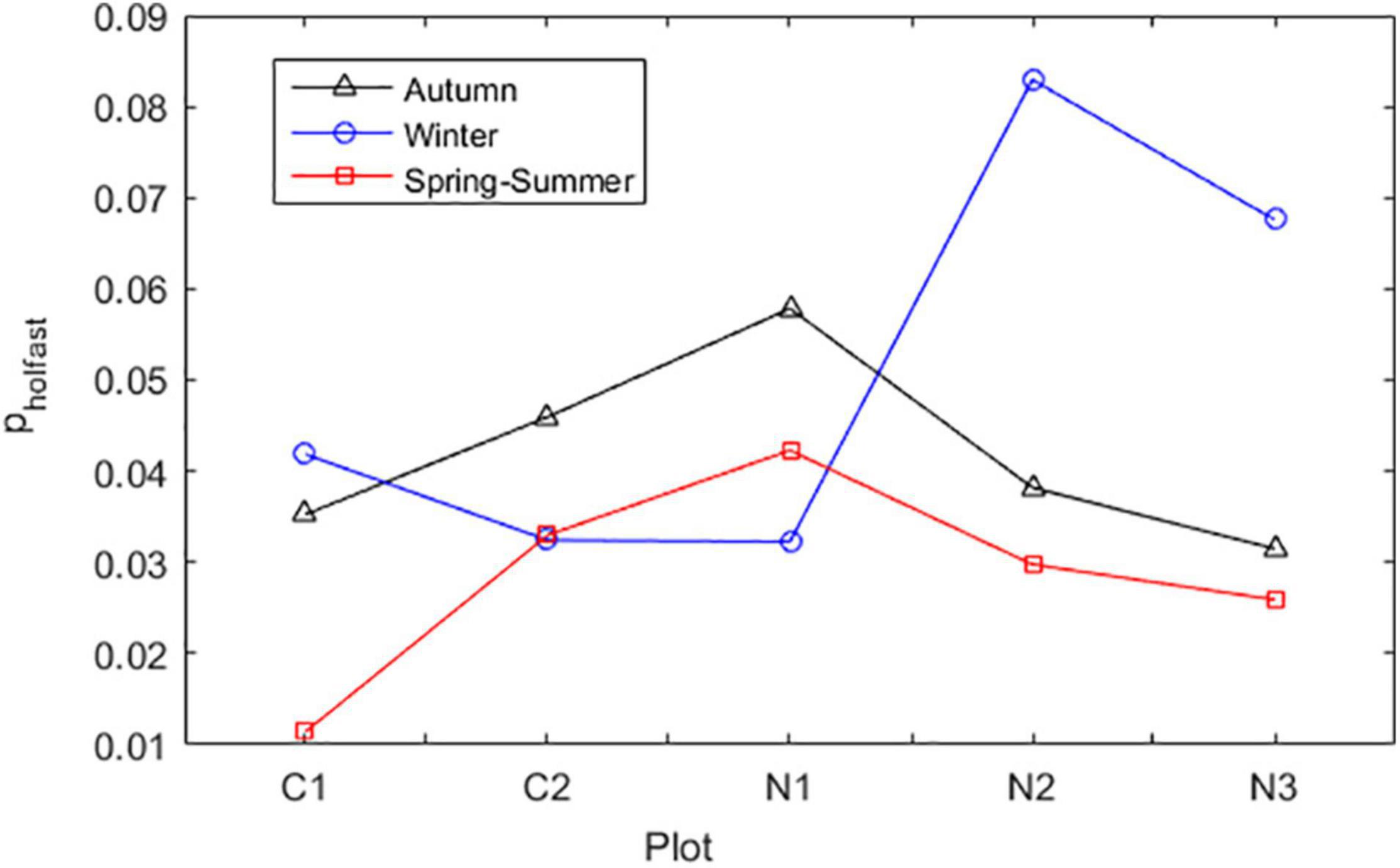
Figure 1. Probability of A. chilense to lose their fronds and survive as bare holdfast (p_holdfast). This probability is dependent on plot and season. Plots were Corral 1 (C1), Corral 2 (C2), Niebla 1 (N1), Niebla 2 (N2), and Niebla 3 (N3).

Then, we inferred about the growth of new fronds from these bare holdfasts. However, the non-linear growth model applied to ‘regular’ fronds could not be applied to the bare holdfasts because of their initial frond volume v = 0. Instead, it was fit the linear form Δv = v_final-v_initial. The results showed that, during the 4-month interval between census, the bare holdfasts endured two distinct faiths (Figure 2). The ones showing Δv < 6 cm³ mainly corresponded to individuals that either did not grow their fronds or grew but broke back again. Their growth was better fit by a Poisson distribution. The ones showing Δv > 6 cm³ corresponded to holdfasts that grew their fronds without breaking. Their growth was better fit by the average between the Burr and the Inverse Gaussian distributions. The dynamics governing these faiths depended on season and location. The bare holdfasts grew less and broke more during winter and/or at C2. In fact, during winter at C2, most of the bare holdfasts broke, and the few ones that didn’t, grew little. At all other plot besides C2, and during spring, summer, and autumn, the growth of the bare holdfasts was also dependent on the plot density (V): the smaller the frond density the lesser these holdfasts regrew their fronds and the more did their regrown fronds broke back (Figure 2). A similar negative correlation was found between the plot density (V) and the survival of the A. chilense individuals monitored during this survey (Vieira et al., 2016, 2018a). This negative correlation is called “Allee effects.” In algae, it occurs because denser alga turfs are more efficient at reducing drag, and thus protecting from hydrodynamic stress tearing the fronds, are more efficient at filtering excess radiation and are more efficient at retaining water when emerged, thus protecting better against desiccation and UV stress (Hay, 1981; Padilla, 1984; Taylor and Hay, 1984; Scrosati and DeWreede, 1998). For the IBM implementation, a random vector (ζ) uniformly distributed within [0 1] was generated with one entry for each bare holdfast. The inverse cumulative density function of the desired probability distribution was applied to transform ζ into Δv.

FIGURE 2

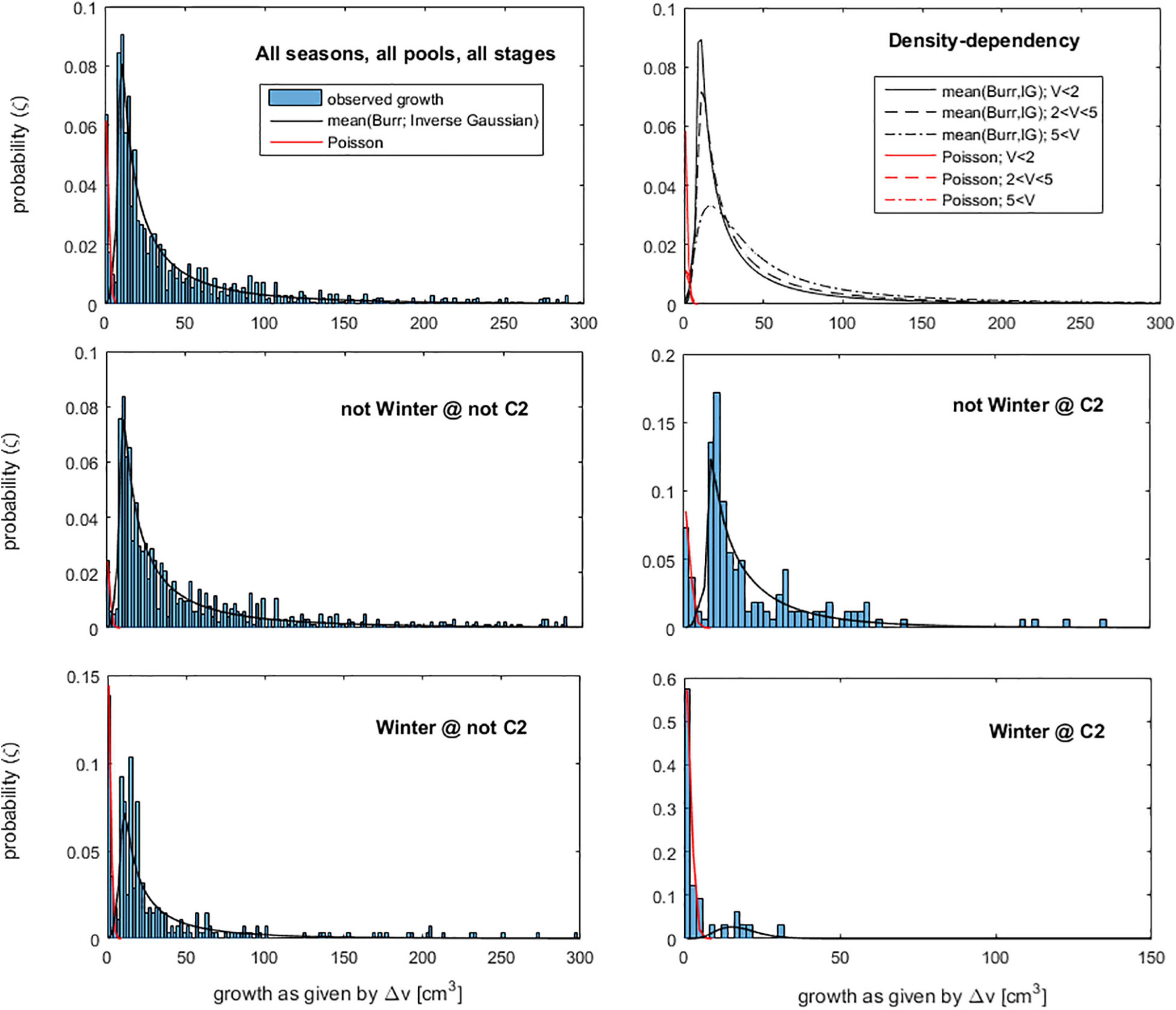
Figure 2. Probability density functions (PDF) of the growth (Δv) of the bare holdfasts. The probability was named ‘ζ’ to avoid confusion with another use of the letter p in this same section. Each panel is the PDF of Δv given the conditions specified in the panel tittle. The surviving bare holdfasts growing less than 6 cm³ were fit by the Poisson distribution. The surviving bare holdfasts growing more than 6 cm³ were fit by the mean of the Burr and Inverse-Gaussian distributions. For density-dependency effects, the PDF of Δw depends on the density of frond volumes (V) on the respective plots.

The probability (p) of a bare holdfast growing less than 6 cm³, and therefore being modeled by the Poisson distribution, was estimated. The opposite probability of a bare holdfast growing more than 6 cm³, and therefore being modeled by the Burr and Inverse-Gaussian distributions, was given by 1-p. This probability was compared among seasons, plots and life-cycle stages (Figure 3) applying a 3-way permutation test with 10,000 randomizations. The test found significant differences among seasons (p = 0.0001) and plots (p = 0.0085), but not among stages (p = 0.93). Post-hoc tests showed that only winter was systematically significantly different from the other seasons, and only C2 was systematically significantly different from the other plots. Interaction effects were not significant. For the initial IBM implementation, a threshold α was set for each of the combinations ‘winter at C2’ (α = 0.7879), ‘winter at all other plots’ (α = 0.1922), ‘spring–summer and autumn at C2’ (α = 0.1227) and ‘spring–summer and autumn at all other plots’(α = 0.0354). The subsequent IBM calibration and validation highlighted the need to model α with more detail. A winter α was estimated for each plot, leading to ‘winter at C1’ α = 0.196, ‘winter at C2’ α = 0.788, ‘winter at N1’ α = 0.362, ‘winter at N2’ α = 0.044 and ‘winter at N3’ α = 0.333. The α was simulated in the IBM as follows: in the column-vector A, with an entry for each individual, were stored the α given by each individuals’ season × plot situation. Then, in the column-vector P, with the same size of A, were stored the p randomly generated from a uniform distribution within [0,1]. All surviving bare holdfasts for which p < α grew less than 6 cm³ and had their growth simulated by the Poisson distribution. All surviving bare holdfast for which p > α grew more than 6 cm³ and had their growth simulated by the Burr and the Inverse Gaussian distributions.

FIGURE 3

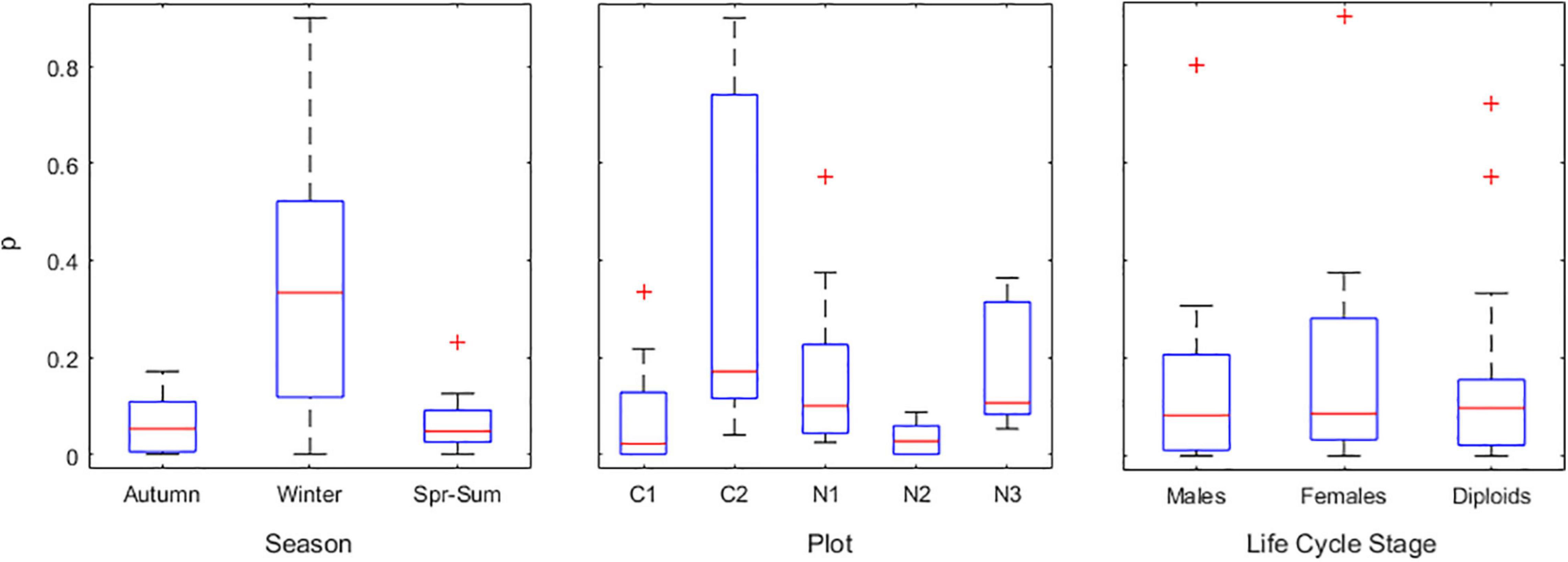
Figure 3. Probability (p) of a surviving bare holdfast growing less than 6 cm³, and therefore being modeled by the Poisson distribution. This probability was estimated for each season (‘Spr-Sum’ refers to spring–summer), each plot and each stage. Plots were Corral 1 (C1), Corral 2 (C2), Niebla 1 (N1), Niebla 2 (N2), and Niebla 3 (N3). Box and whiskers represent the quartiles, and the red ‘+’ symbol represents outliers.

Fertility

To estimate whether each individual was fecund or not (1 or 0), was generated a random vector (P – ‘Rho’) uniformly distributed within [0,1], with an entry for each individual alive. In parallel, the probability of each individual being fecund was estimated depending on the states of its individual properties and stored in another vector (ρ – ‘rho’) of equal size. All individuals for which P ≤ ρ were fecund (1). Otherwise, they were not (0). The algorithm for this probability of being fecund was presented by Vieira et al. (2018b). The general pattern was that the spring–summer season was when less diploids and haploid females were fecund. Only the haploid males managed to maintain their ρ high throughout the yearly cycle. For the current application, the ρ estimation from Gompertz curves was re-calibrated using the algorithm by Vieira (2020). The difference noteworthy was the ρ estimation for diploids in Corral during spring–summer (Supplementary Figure 4). We assume that the extreme survival probability of the few largest diploids in Corral during spring–summer was an outlier due to the small number of observations (n = 7). This detail was insignificant for posterior IBM validation.

The spore production by fecund individuals (f) was dependent on their frond volumes (v) so that f = f_v⋅v. The f_v was the spore production per cm³, dependent on season and location. The IBM calibration and validation highlighted the need to include more detail in the f_v estimation than the previous algorithm by Vieira et al. (2018b). Permutation tests with 10,000 randomizations applied to log₁₀(f_v) showed that tetraspore production was significantly different among seasons (p = 0.0232) and among plots (p = 0.0003), with interaction effects being also significant (p = 0.0001). Carpospore production was significantly different among seasons (p = 0.0001) and among plots (p = 0.0001), with interaction effects being also significant (p = 0.0001). The simplest solution was to use the spore production specific to each plot × season combination (Supplementary Figure 5). The spore production was generally lower during spring and in Corral. This was always true for the carpospores. The exception was the production of tetraspores in Corral, which actually increased in the spring.

Both the production of reproductive structures and the production of spores was lower during the spring–summer, and particularly at Corral. Several factors may have contributed to this general pattern: October corresponds to the austral spring, when the sun is higher, the daylength is larger, and intertidal stands are more exposed to stress from desiccation and UV radiation. Corral was where fronds lay and dry on the flat bare rock during low tide (see Supplementary Figure 1 in Vieira et al., 2021). If A. chilense is conditioned to enhance its resource allocation in costly metabolites that help withstand desiccation and UV stress, these used resources lack for everything else, including for the production of spores. Furthermore, the October (spring) census followed the winter season, during which it is reasonable to assume that A. chilense stands at high latitudes were light-limited and thus, low on energy reserves, as suggested by their decreased growth (Vieira et al., 2021). Therefore, A. chilense fronds enter the spring–summer season with smaller sizes (their reproduction is proportional to size), low on energy reserves and having to spend a significant part of their energy budget in protection from desiccation and UV stress.

We were unable to develop a spore survival algorithm and couple it to the IBM. Hence, the fertility properties described above were only used for the validation of this IBM. Alternatively, we developed a recruitment algorithm bypassing spore production and survival (see section “Recruitment” below). The sex ratio of the tetrasporelings at the end of each season was tested (Supplementary Figure 5). Permutation tests with 10,000 randomizations showed that differences were significant between sites (p < 0.0001) but not among seasons (p = 0.0795), and there were no interaction effects (p = 0.2178). We preserved the sex ratio differences between Autumn and the remaining seasons given the low chances of Type 2 error vs. the potential benefit for model accuracy. The sex ratio model was given by the ANOVA linear model%males = μ + α_site + α_season, where μ is the average sex ratio and α are the treatment-specific coefficients.

Recruitment

When recruitment was a forcing function, each IBM iteration was forced with the recruits observed at each plot and census, i.e., adding the observed number of recruits and with their observed sizes. When recruitment was a population property to be solved, the number of recruits of each stage, in each plot and at each new IBM iteration, was estimated from the recruitment algorithm. The strong negative correlation between recruitment and the density of adult fronds (Figure 4) demonstrated that the fundamental factor governing recruitment was competition with adults deterring the viability of settled spores. The fecundity level of adults was of little relevance as they always produced enough spores to sustain recruitment. The level of competition among recruits and adults was affected by year, season and location. These effects were stronger in Corral, where recruits were emersed in the flat bare rock during low tide, exposed to UV and desiccation. In this case, recruitment was larger during the winter. In Niebla, where individuals were always immersed in rock pools, the effects of season and year were milder, while differences among rockpools came to light. Competition with the adults, as well as summer, were more stressful for carposporelings than for tetrasporelings, particularly for those in Niebla. Models used for the recruitment dependency on V were linear, linear relative to log₁₀ recruitment, and exponential. Model type and coefficients were stored in the Par.recruitment array and not supposed to be edited by the user. The low number of observations for some particular cases (often only two) disabled statistical inference. Nevertheless, the posterior IBM validation supports this algorithm.

FIGURE 4

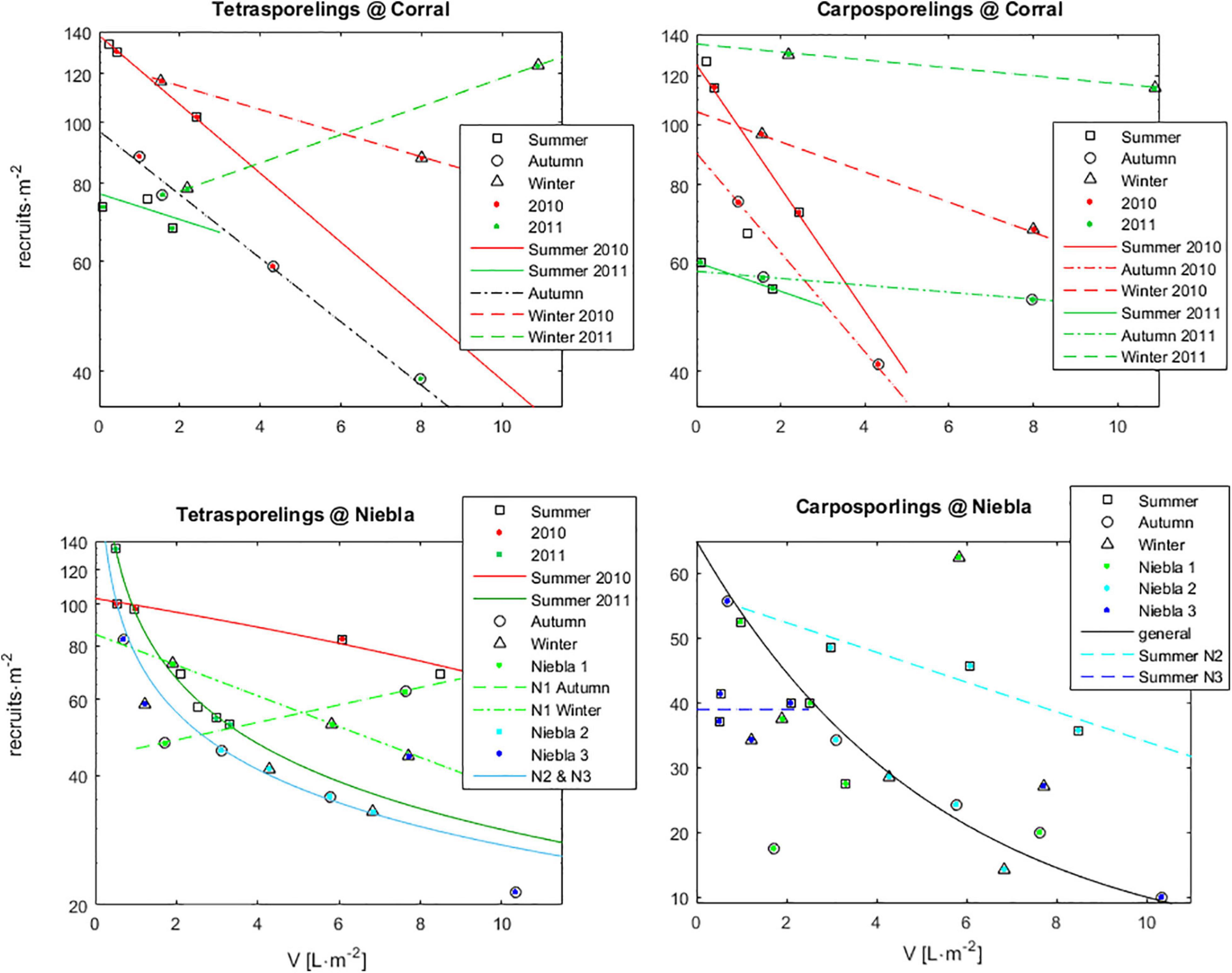
Figure 4. Recruitment algorithm. Recruitment of haploid (Tetrasporelings) and diploid (Carposporelings) germlings at time t, and its dependency on the density of adult fronds (V) at time t-1. Further effects of year, season and location are shown. Plots were Corral 1 (C1), Corral 2 (C2), Niebla 1 (N1), Niebla 2 (N2), and Niebla 3 (N3). Markers represent observations and lines the applied models.

The size of each recruit was estimated from the ANOVA linear model (Equation 2), where μ was the mean log(v), α correspond to the effects of season, plot, stage and their interactions, and ε was the error with distribution N(0,σ).

$\log \left(v\right)=\mathrm{\mu }+{\mathrm{\alpha }}_{season}+{\mathrm{\alpha }}_{pool}+{\mathrm{\alpha }}_{season\cdot pool}+{\mathrm{\alpha }}_{season\cdot stage}+{\mathrm{\alpha }}_{pool\cdot stage}+\mathrm{\epsilon }(2)$

A permutation test with 10,000 randomizations was applied to the 1938 observations of new-borns’ sizes. The dependent variable was the logarithm of their measured sizes, log(v). The factors were season, plot and life cycle stage. The mean log(v) was μ = −0.1053, corresponding to v = 0.9 cm³, and the variance within groups was σ = 2.731. The standard 5% significance threshold was relaxed. The posterior IBM calibration showed how important was the inclusion in the algorithm for the recruits’ size (equation 1) of some α whose respective p values were above the traditional 5% acceptance threshold. There were significant differences among seasons (p < 0.0001), with the size of recruits in October, i.e., after winter (α = −0.526) being significantly smaller than in February, i.e., after summer (α = 0.234) (p < 0.0001) or June, i.e., after autumn (α = 0.134) (p ≤ 0.0001). Since there were no differences between February and June (p = 0.127), their pooled α was used. We highlight that, in this specific case of seasonality, the α estimated with data from one census corresponds to the season starting 4 months earlier. There were significant differences among plots (p < 0.0001), with basically almost all being significantly different. Therefore, we used all α_C1 = 0.271, α_C2 = −0.421, α_N1 = 0.51, α_N2 = 0.826 and α_N3 = −0.203. The diploid new-borns (α = 0.081) were mildly larger than the haploid male new-borns (α = −0.04) and haploid female new-borns (α = −0.075). These differences were found not statistically significant at the 5% threshold (p = 0.117). Nevertheless, we used them as they match previous evidence, here and elsewhere (Guillemin et al., 2013; Vieira et al., 2018b), that the sole diploid advantage in the A. chilense life cycle occurs in the survival and growth of spores and sporelings, and that this advantage likely comes from maternal care by their haploid female progenitors (Kamiya and Kawai, 2002). There were interaction effects between season and plot (p = 0.0015). By the end of summer, new-borns at Corral had enhanced sizes (α = 0.215, p = 0.005 and α = 0.105, p = 0.053) whereas new-borns at Niebla had diminished sizes (α = −0.151, p = 0.128, α = −0.339, p = 0.0001 and α = −0.238, p = 0.0003). After winter, on the contrary, new-borns at Corral 2 had diminished sizes (α = −0.216, p = 0.006) whereas new-borns at Niebla rock pools had enhanced sizes (α = 0.349, p = 0.091, α = 0.587, p = 0.032 and α = 0.245, p = 0.069). There were interaction effects between season and stage (p < 0.0001). Haploid male new-borns had diminished sizes by the end of Autumn (α = −0.341, p = 0.005), and enhanced sizes after winter (α = 0.218, p = 0.056). For this same survey, Vieira et al. (2021) previously reported that the haploid males were the only not decreasing frond growth during winter. Haploid female new-borns had enhanced sizes by the end of autumn (α = 0.226, p = 0.027). There were interaction effects between plot and stage (p < 0.0001). At the Niebla 3 pool, haploid male new-borns were smaller (α = −0.275, p = 0.012) and diploid new-borns were larger (α = 0.249, p = 0.019). Haploid female new-borns were smaller at the Niebla 1 pool (α = −0.324, p = 0.087).

Model Output

Several estimated individual and population properties were fundamental for model calibration and validation, as well as posterior analysis of A. chilense demography. These included properties estimated and applied during model simulation (abundances, sizes, recruitment, etc.) and properties estimated but not applied during model simulation as the ratio of haploids to diploids (H:D). Simulated and observed properties are plotted for calibration and validation. The user chooses whether or not to plot the default figures in Properties_Fig.m child script. Furthermore, it is also possible to choose whether to arrange the plots horizontally (landscape) or vertically (portrait), and the colors, markers and line styles.

Results

The first step of the A. chilense IBM calibration and validation addressed the individual properties related with the fate of the fronds, namely, their survival, growth and breakage, and temporarily leaving aside the fertility properties. For that, each IBM iteration was forced with the observed recruitment. The calibration and validation used the eight census of the experiment (sim.year = 2009, sim.month = ‘Oct’ and timespan = 2.8). The age of the individuals already present at the beginning of the experiment was unknown, and inference from their size was impossible since the generalized occurrence of frond breakage disrupted any age-size correlation. Attributing them the rounded average population age (8 months) provided good results. The IBM replicated well the observed population properties (Figure 5). Having disregarded yearly variability in the calibration of survival and growth parameters was the main source of error in the predictions. The best estimations of abundances and of the H:D demanded improved estimations of the stand volume (V) which, in its turn, were only possible from improved frond growth and breakage algorithms, together with the inclusion of the holdfast algorithm. The former algorithms by Vieira et al. (2021), relying exclusively on results deemed statistically significant, despite a data set as large as 6,066 observations, failed to capture the growth dynamics with sufficient detail and precision for the current IBM application.

FIGURE 5

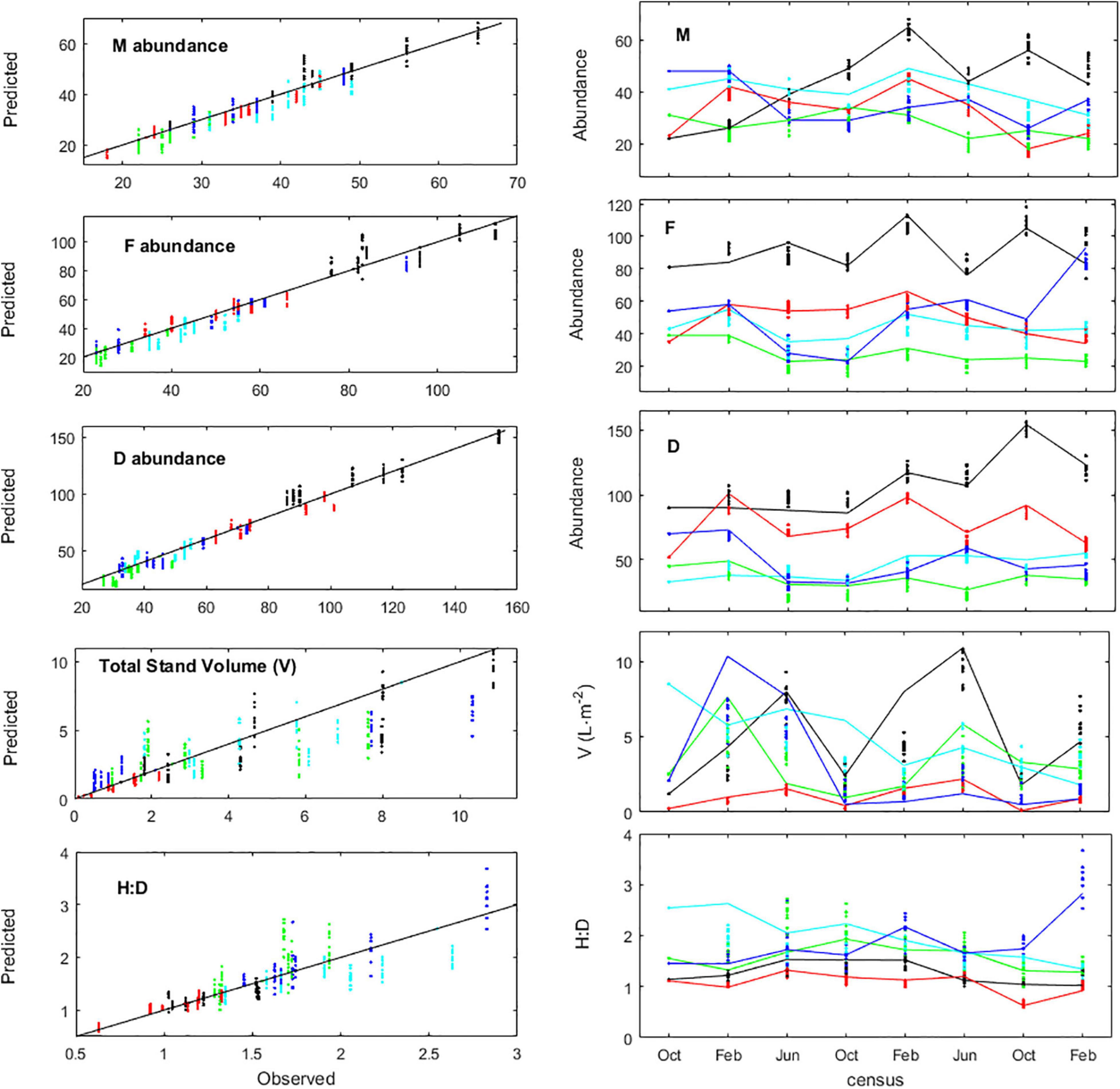
Figure 5. Agarophyton chilense IBM calibration and validation from estimates of population properties, namely, abundances of males (M), females (F) and diploids (D), frond density (V) and haploid-to-diploid ratio (H:D). Observed properties compared against properties predicted from 10 runs of the IBM. Population properties estimated for plots Corral 1 (black), Corral 2 (red), Niebla 1 (green), Niebla 2 (light blue), and Niebla 3 (dark blue). Observations during February (Feb), June (Jun), and October (Oct). Left panes: standard (predicted:observed) plots with 1:1 gray solid line. Right panes: time series with observations (solid lines) and estimates (colored dots).

The calibration and validation of the frond growth and breakage algorithms was a particularly complex task given the simultaneous occurrence of both fates, and the apparent randomness with which fronds broke and by how much did they brake. Consequently, it was not possible to compare the sizes observed and estimated for each individual at each census. Alternatively, sizes were ranked and compared among similar rank, i.e., largest estimated against largest observed, second largest estimated against second largest observed, and so forth. Since observed and estimated numbers of individuals alive did not matched, to the smaller set of individuals (observed or estimated), the individuals lacking were added with a frond size of 0.001 cm³ arbitrarily attributed; which is slightly below the smallest frond (0.006 cm³) measured during the experiment. This procedure showed that the IBM generally replicated well the distributions of frond sizes (Figure 6).

FIGURE 6

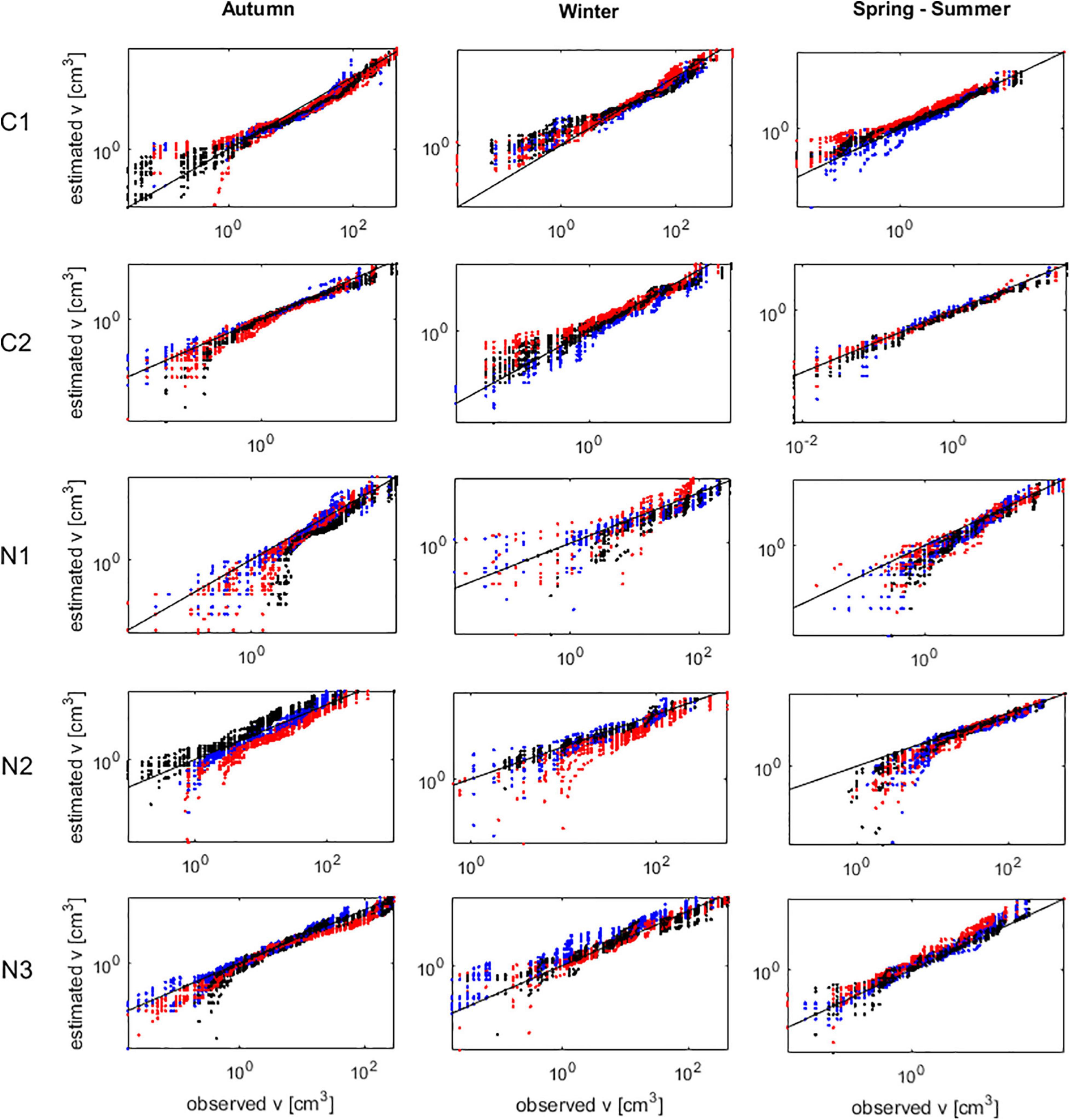
Figure 6. Agarophyton chilense IBM calibration and validation of frond size (v) estimates. Observed size compared against size predicted from 10 runs of the IBM. Oblique black lines represent the 1:1 line identifying the perfect match between predictions and observations. Male haploids (blue), female haploids (red), and diploids (black). Plots were Corral 1 (C1), Corral 2 (C2), Niebla 1 (N1), Niebla 2 (N2), and Niebla 3 (N3).

Stands were generally haploid-dominated, with the H:D tending to be more even at Corral and more uneven at Niebla (Figure 7A). Rocky platform C2, despite being the environmentally harsher, generally exhibited higher abundances of females and diploids than the Niebla rock pools. However, these females and diploids were mainly recruits or young individuals that did not survive for long (5.26 months on average) nor grew large (2.76 cm³ on average) (Figure 6). On the other hand, females and diploids in Niebla generally grew older (6.36 months on average) and larger (9.3 cm³ on average) (Figure 6). The recruits’ H:D (i.e., initial forcing to the IBM) and the stand H:D simulated by the IBM at each iteration were not much different (Figure 7A). The recruits’ H:D was approximately the central tendency to the stands’ H:D. Nevertheless, the H:D varied with A. chilense’s age, becoming more uneven among older individuals (Figure 7B). At Niebla, the ≈1.8 H:D of the younger raised only slightly to the ≈1.9 H:D of the older. Changes were stronger at Corral, where the ≈1.1 H:D of the younger raised to the ≈1.6 H:D of the older.

FIGURE 7

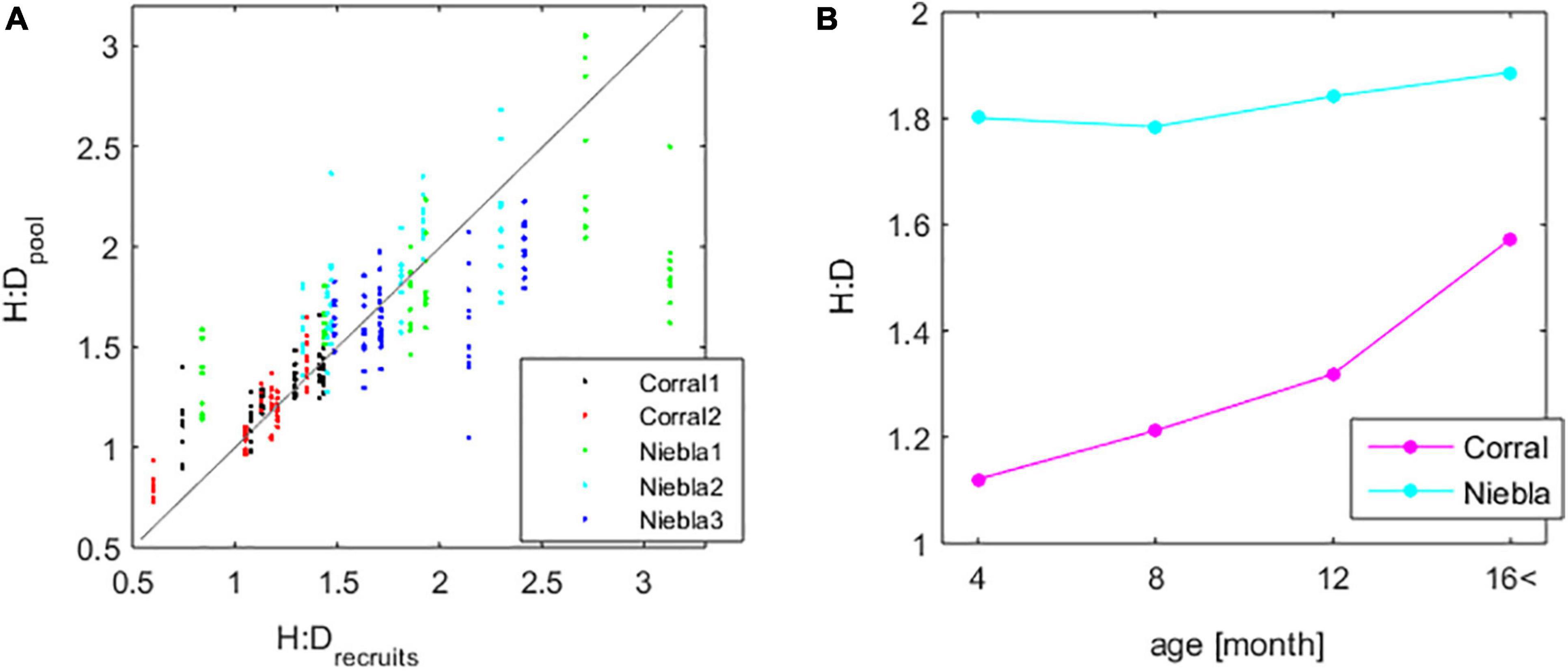
Figure 7. Effect of the age-structure of the population on the haploid-to-diploid ratio (H:D): (A) HD of the recruits (i.e., imposed as forcing function) and the resulting population H:D simulated by the IBM. The gray line represents the 1:1 match. (B) H:D evolution with age of the cohort.

The final step was to calibrate the fertility algorithms and validate the IBM run in full mode, i.e., with recruitment estimated from the population properties (see section “Recruitment”). Although its accuracy inevitably decreased, it still replicated well the abundances, biomass, H:D (Figure 8) and frond size. This is noticeable given that fertility is the factor often causing algal demographic models to fail. The observed and predicted ploidy phase dominance generally matched. The few cases where it did not were always situations where it was almost even – i.e., the H:D close to 1 – and the shift in ploidy dominance still represented minor changes in the H:D. The IBM run in full mode preserved the larger haploid dominance in Niebla and the episodic diploid dominance in Corral 2 during spring–summer.

FIGURE 8

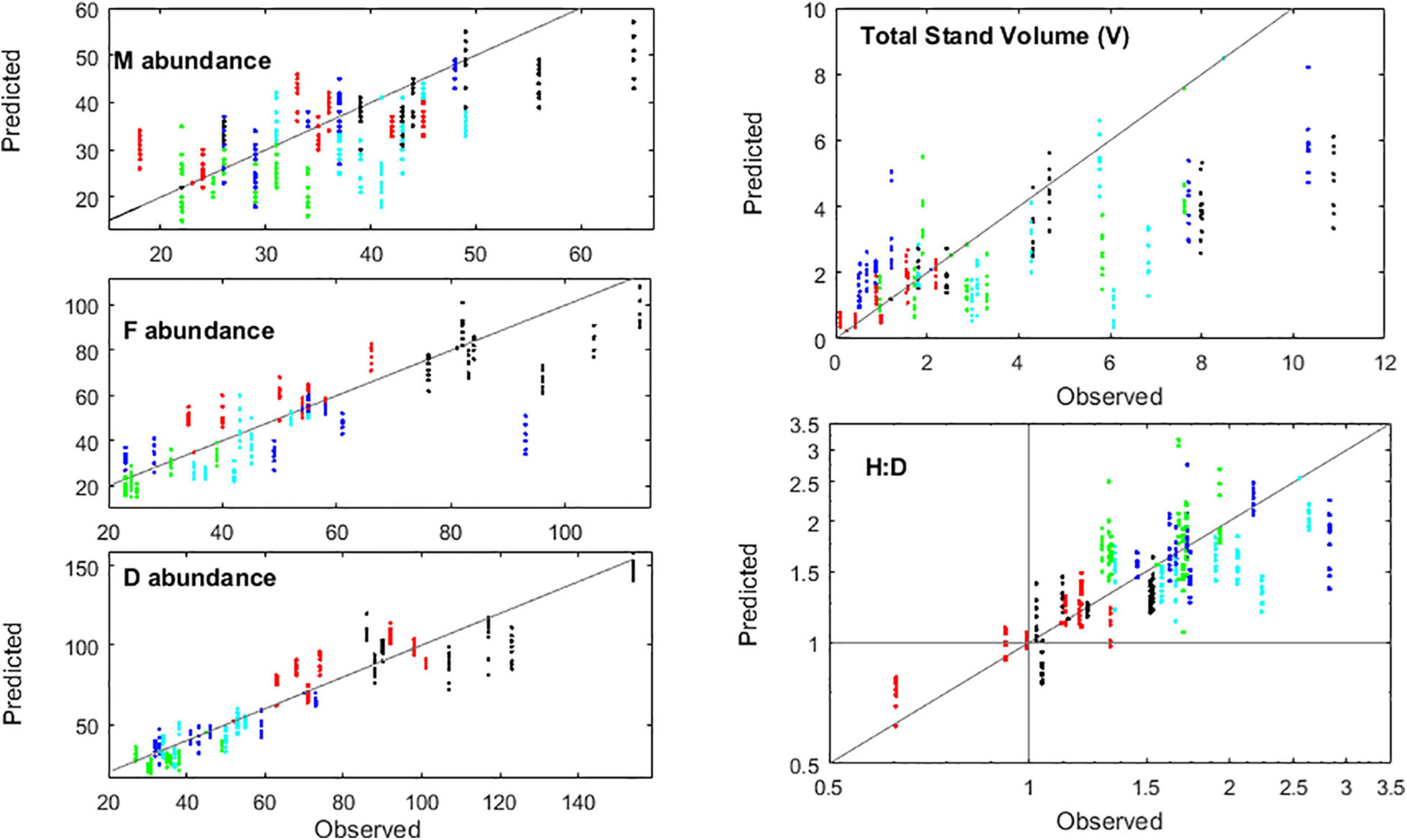
Figure 8. Validation of the IBM run in full mode, based on the predicted abundances of males (M), females (F) and diploids (D), on the total volume of fronds per m² of algal stand (V), and the ratio of haploids to diploids (H:D). Markers represent plots Corral 1 (black), Corral 2 (red), Niebla 1 (green), Niebla 2 (light blue), and Niebla 3 (dark blue). The H:D plot in a log scale represents better the H:D dynamics (see Vieira et al., 2021).

The IBM also replicated well the A. chilense fertility dynamics. The forecasted probabilities of fronds becoming fecund, as well as the forecasted production of carpospores and of tetraspores, showed good agreement with observations (Figure 9). Only the male fertility was not so well replicated. The algorithm for diploid recruitment was the more accurate (Figure 10) since it did not have the sex ratio estimation acting as additional source of uncertainty. The quality of the recruitment algorithm was fundamental for the IBM accuracy, as shown by the correlation between biases in recruitment and abundances (Figure 11). This is expected for most algal demographic models, given the high fertilities, high mortalities and low generation times of most algal life cycles. The negative correlation between recruitment and stand biomass V (see section “Recruitment”), due to competition, generated a negative feedback that was fundamental for the IBM stabilization and therefore, for the stabilization of the A. chilense demography.

FIGURE 9

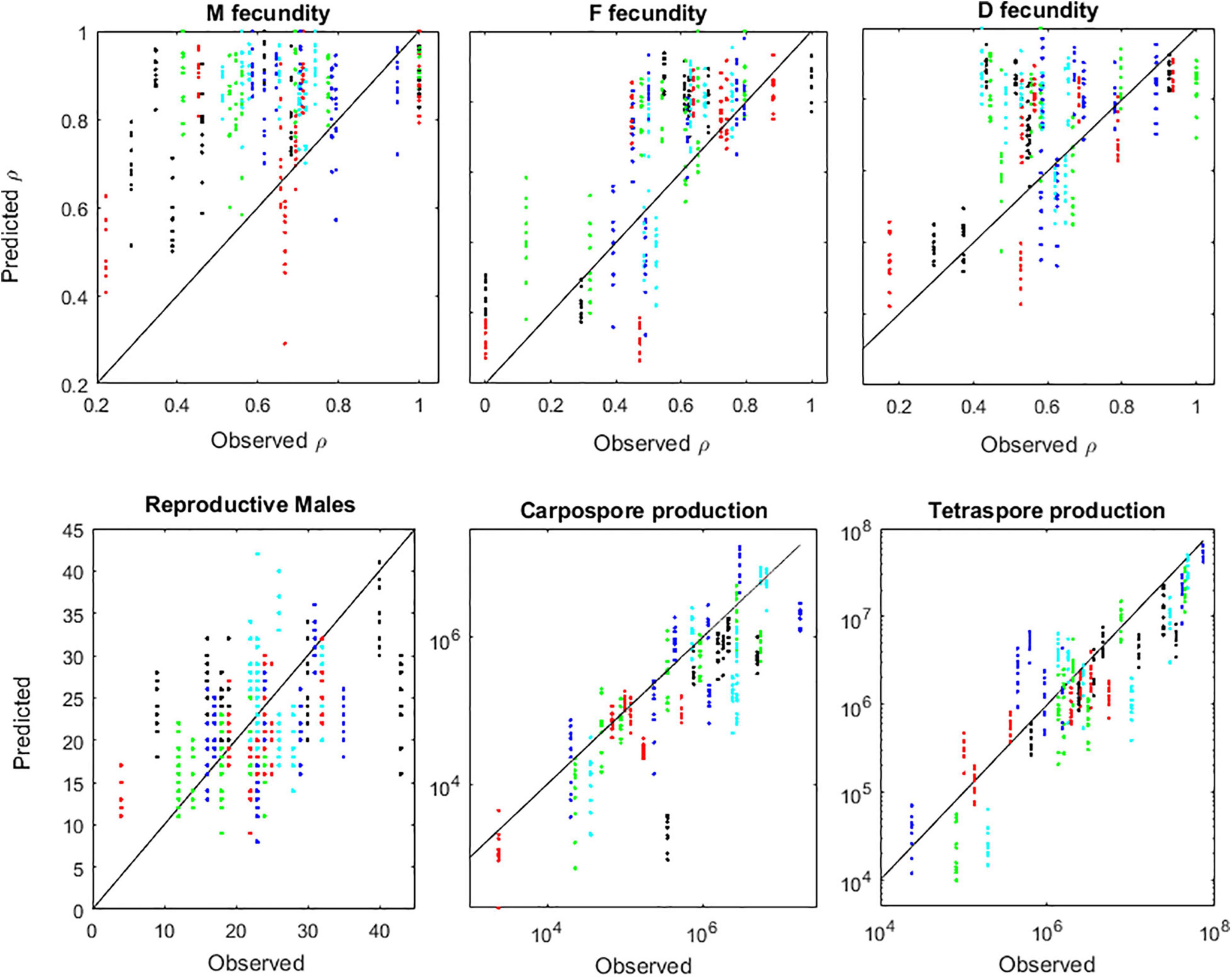
Figure 9. Validation of the IBM run in full mode. Upper panels: comparison between observed and predicted probabilities (ρ) of males (M), females (F), and diploids (D) becoming fecund. Bottom panels: observed and predicted numbers of reproductive males, and the total production of carpospores and tetraspores. Markers represent plots Corral 1 (black), Corral 2 (red), Niebla 1 (green), Niebla 2 (light blue), and Niebla 3 (dark blue).

FIGURE 10

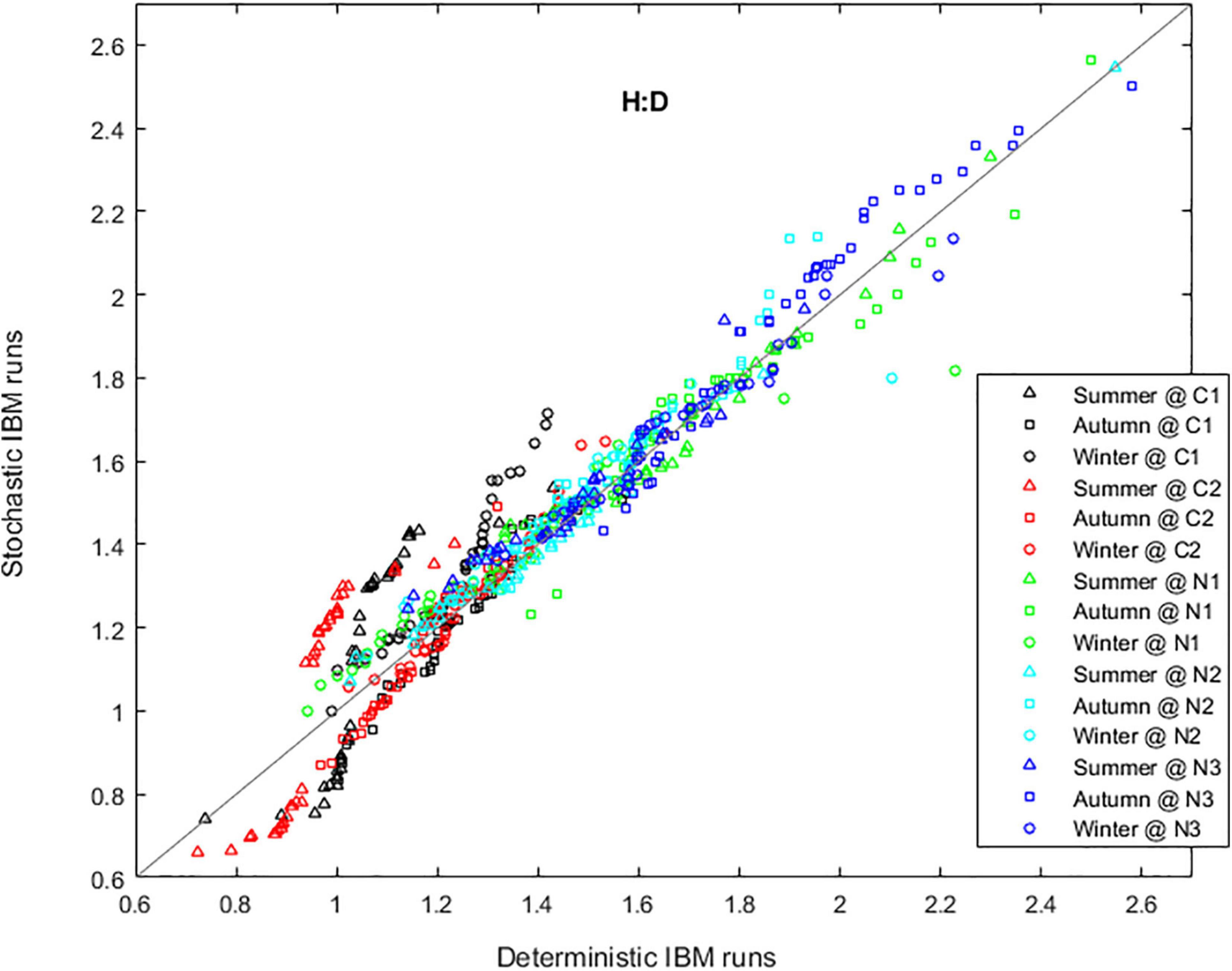
Figure 10. Comparison between deterministic and stochastic runs of the IBM based on the forecasted haploid-to-diploid ratio (H:D) in plots Corral 1 (black), Corral 2 (red), Niebla 1 (green), Niebla 2 (light blue), and Niebla 3 (dark blue) during summer, autumn, and winter. Simulations of 20 years, starting October 2009. Simulations are stochastic or deterministic from February 2012 onward.

FIGURE 11

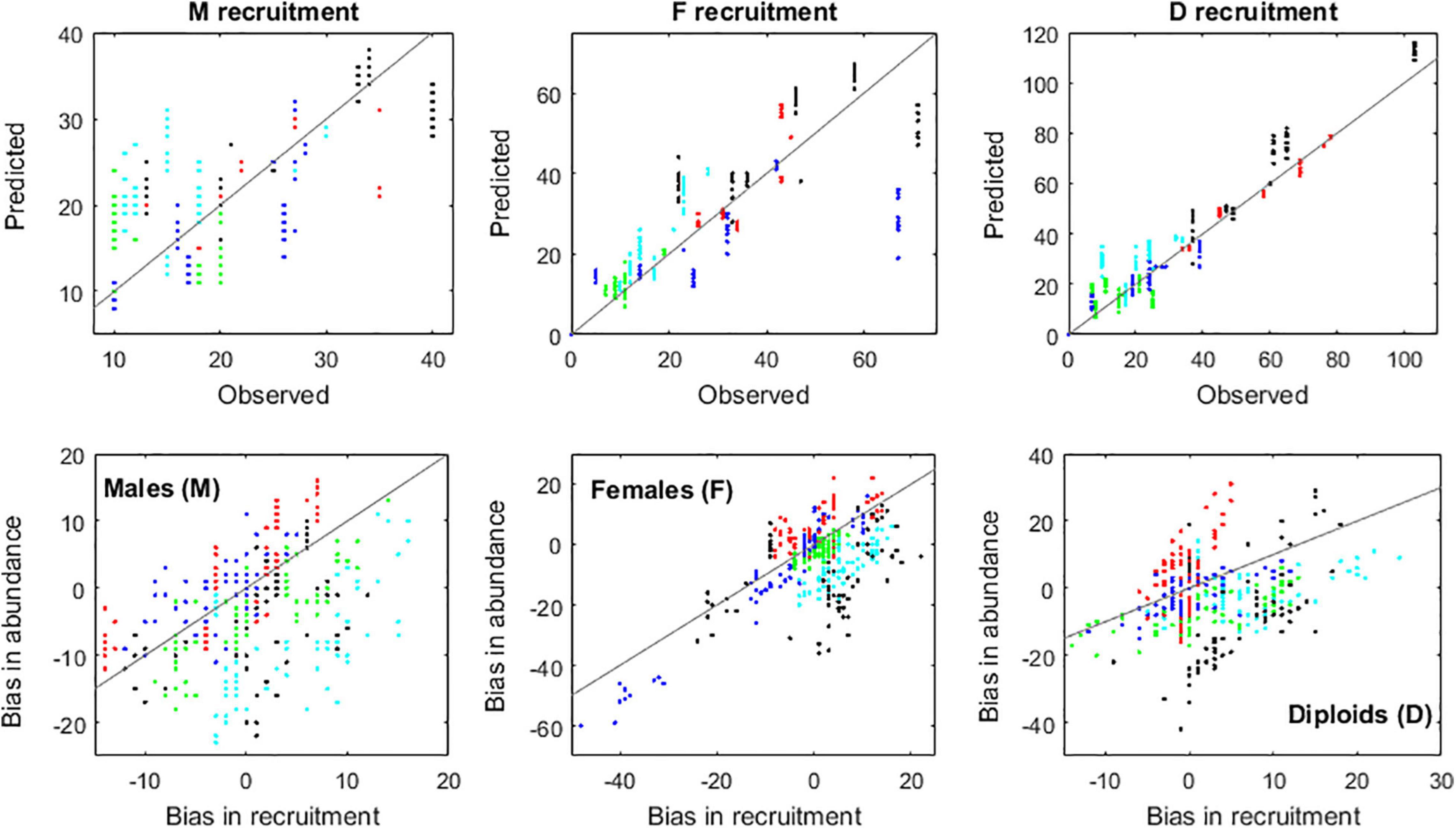
Figure 11. Validation of the recruitment algorithm. Upper panels: comparison between observed and predicted recruitment. Bottom panels: Impact of the recruitment algorithm on the IBM performance. Markers represent plots Corral 1 (black), Corral 2 (red), Niebla 1 (green), Niebla 2 (light blue), and Niebla 3 (dark blue).

The algorithms and coefficients developed from data sufficed to calibrate the IBM well enough to favor it with accuracy as well as long-run stability (Figure 12). No artificial numerical controls were required. This enabled to rely on long runs of the IBM to draw conclusions about the demography of intertidal A. chilense stands. The results from 10-year runs of the IBM (sim.year = 2009, sim.month = ‘Oct,’ timespan = 10 and projection_type = stochastic) confirmed that survival in this species is always low. Consequently, mean age was 207, 159, 226, 222, and 221 days, respectively, in Corral 1, Corral 2, Niebla 1, Niebla 2, and Niebla 3 plots. During spring–summer, A. chilense decreases fecundity, diverting its focus to growth. Nevertheless, some fertility was preserved as, with such high mortalities and short generation times, these populations cannot afford too long without reproduction. During winter, A. chilense shifts its focus to fecundity, decreasing growth (see sections “Frond Growth” and “Fertility,” and Vieira et al., 2018b,2021). The seasonal ramet ecophysiology resulted in relatively stable seasonal oscillations of the population’s properties, namely the abundances, biomass, fertility and H:D (Figure 12). In Niebla the H:D is more stable and always biased toward haploids, ranging from 1 to 3 but most often within 1.2 and 2. It usually peaks in the autumn due to increased abundances of the haploids. In Corral the H:D is more unstable. It is usually mildly diploid-biased relative to the H:D≈1.4; most often within 0.9 and 1.5. However, some years, during the spring–summer, it shifts to a clearer diploid dominance, ranging within 0.5 and 0.9. These occur on the account of spring–summer peaks in diploid abundance. Pluriannual oscillations also occurred. Simulations ranging 20 years (not shown) showed conspicuous occurrence of H:D oscillations in Corral with diploid dominance peaking in the spring–summer at periods of 1, 2 and 3 years. This resulted from the random pairing of favorable or unfavorable years. Abundances are systematically larger in Corral than in Niebla. However, this does not mean that the environmental conditions are better in Corral than in Niebla. There is still the quality of the individuals composing those abundances, i.e., their set of individual properties. In Corral 2, where survival is outstandingly lower, the larger abundances pertain to young individuals with small fronds that sum to little stand biomass. In the relatively more survival-oriented Niebla rock pools, the lower abundances pertain to older individuals with larger fronds that sum to greater stand biomass. This aspect of the A chilense demography resembles classical theories and dynamics of general ecology, namely, the r-strategist vs. K-strategist duality in demography, the self-thinning law, and the plants’ ecological succession from pioneer communities (prairies) to climax communities (woods). In the more survival-oriented Niebla rock pools the H:D is stable along the population’s age structure. In the relatively less survival-oriented Corral rock platforms the H:D shifts along the population’s age structure. This shift goes from recruits following the H:D set by the ploidy differentiation in fertility, to the elder following the H:D set by the ploidy differentiation in growth and survival.

FIGURE 12

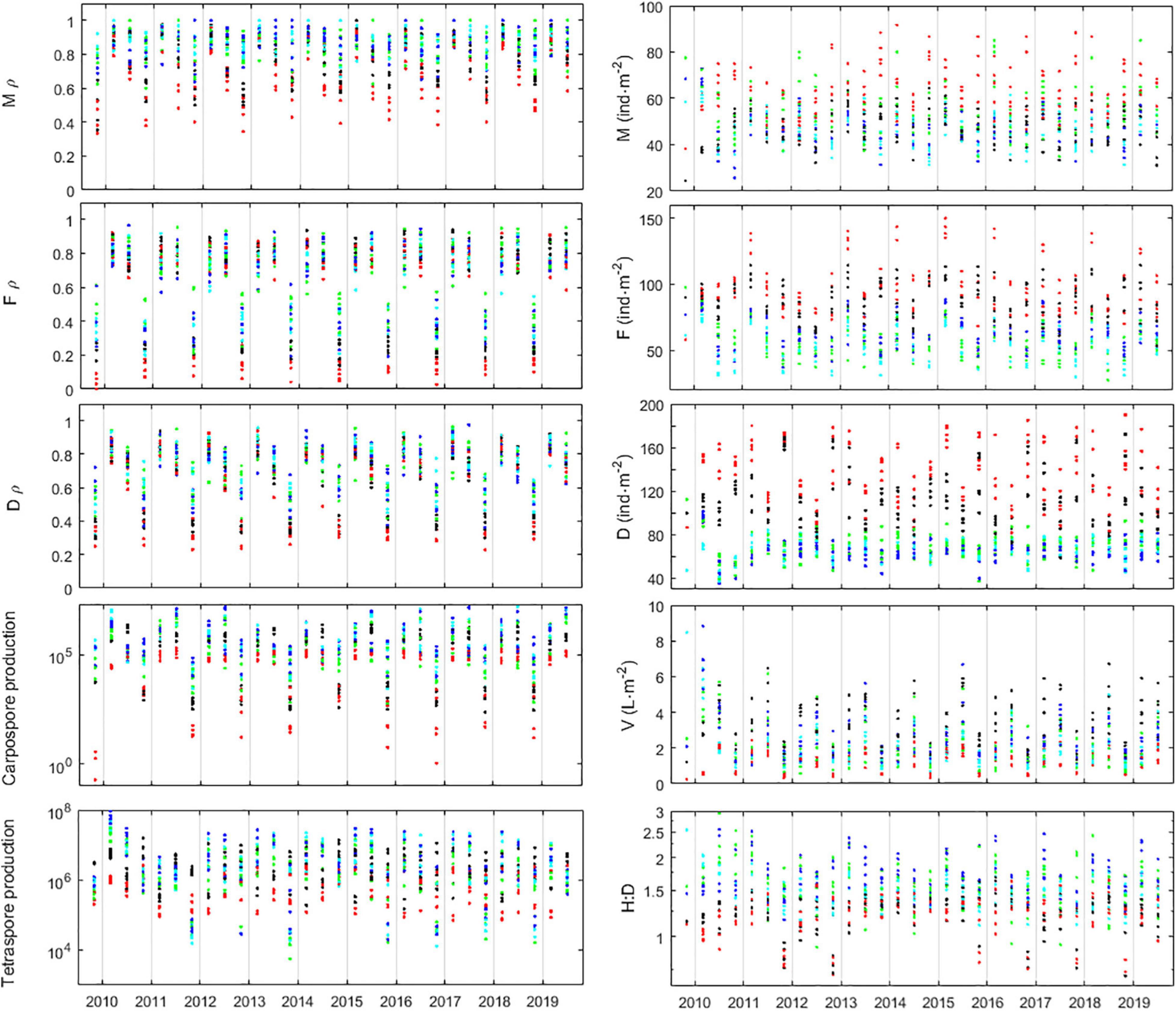
Figure 12. Simulations of the A. chilense demography using the full IBM. Left panels show the fertility properties, namely, the probabilities (ρ) of males (M), females (F), and diploids (D) becoming fecund and the productions of tetraspores and carpospores. Right panels show the abundances of males (M), females (F), diploids (D), stand bimass density (V), and ratio of haploids-to-diploids (H:D). Five runs of the IBM are shown, simulating 10 years, starting October 2009. Simulations are stochastic from February 2012 onward. Markers represent plots Corral 1 (black), Corral 2 (red), Niebla 1 (green), Niebla 2 (light blue), and Niebla 3 (dark blue).

The interannual variability in recruitment was more evident at the harsher Corral location, enhancing the ploidy differentiation in niche occupation. To demonstrate it, were performed IBM runs simulating 20 years. The deterministic runs, by disregarding interannual variability (see section “Simulation Properties” point h), smoothed the H:D forecasts. On the contrary, the H:D forecasted by stochastic runs was more biased toward one of the phases, depending on the year-specific conditions (Figure 10). This was more evident in Corral, where the inter-annual variability in winter recruitment led to a spring–summer H:D that alternated from more biased toward the haploids to more biased toward the diploids.

To understand better the effects of seasons on the A. chilense demography, the IBM was run as if there was always the same season. To avoid bias from the effect of inter-annual variability, deterministic 20-year-long runs of the observed seasonality were compared with deterministic 20-year-long runs of always autumn, always winter or always spring–summer (Figure 13). If it was always autumn, abundances would tend to be lower due to lesser recruitment. The population would shift to older and larger individuals, summing to larger stand volumes (V). The H:D would be similar among Corral and Niebla stands and more stable around the theoretical H:D≈1.4. Thus, if it was always autumn, there would not be much of a difference between haploids and diploids. If it was always winter, abundances would be higher due to larger recruitment. The population would have younger and smaller individuals, summing to smaller stand volumes (V). The H:D would be less biased toward the haploids and completely separated among sites. In fact, the H:D at Corral would become always diploid-dominated while at Niebla, would keep on being always haploid-dominated. If it was always spring–summer, the abundances of the haploid females would be higher, whereas the abundances of the diploids would be lower. Consequently, the H:D would always be dominated by the haploids.

FIGURE 13

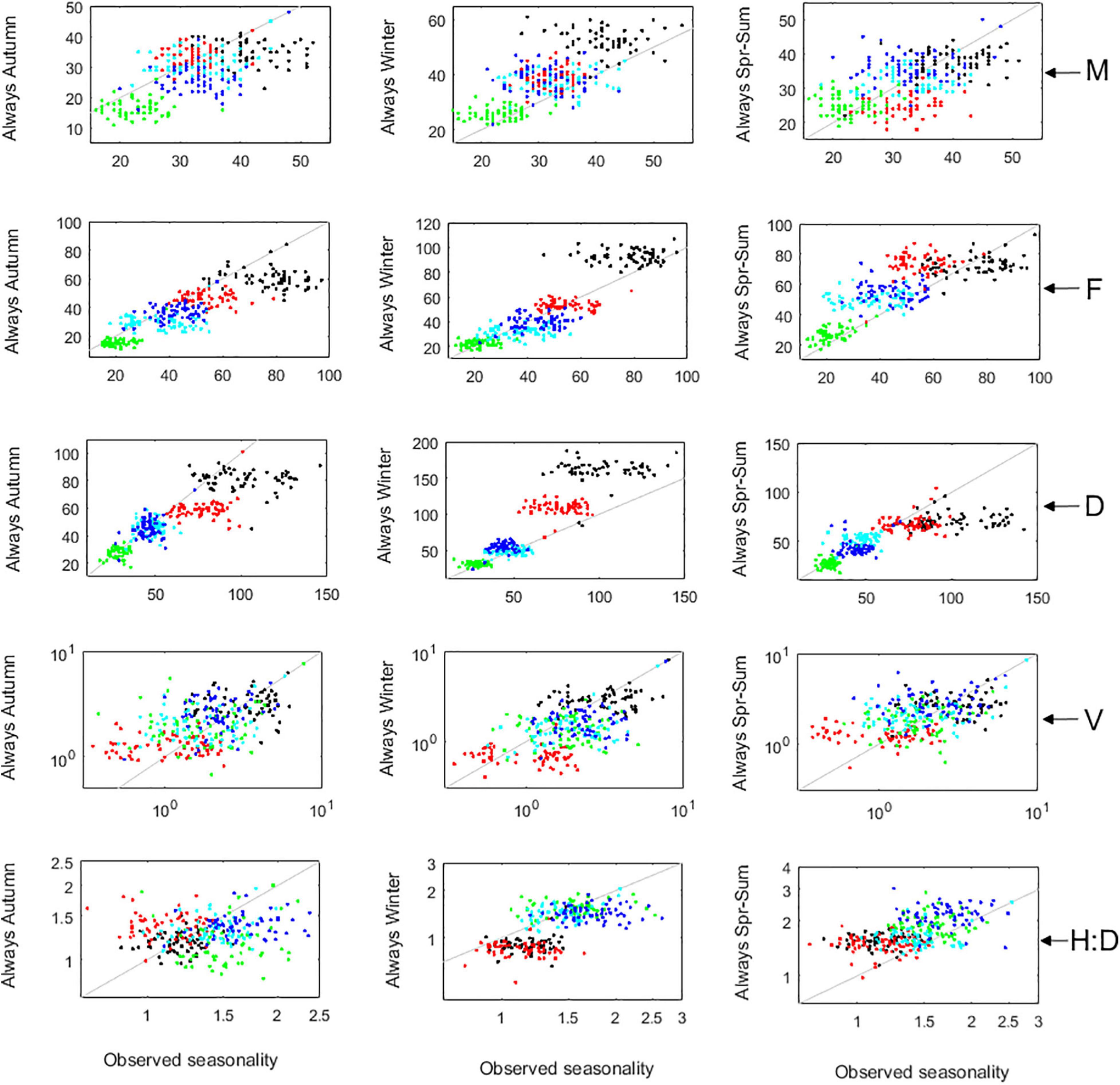
Figure 13. The effects of seasons on the demography of A. chilense. Comparison between observed seasonality and the predicted algal stand if it was always the same season. M, F, and D are the abundances of males, females, and diploids, respectively. V is the total frond volume per square meter. H:D is the ratio of haploids to diploids. Markers represent plots Corral 1 (black), Corral 2 (red), Niebla 1 (green), Niebla 2 (light blue), and Niebla 3 (dark blue). Gray line represents the 1:1 line.

Discussion

The conditional differentiation between haploids and diploids leading to their niche partition was theoretically tested and advanced as the cause for the evolutionary stability of isomorphic biphasic life cycles (Hughes and Otto, 1999). Our work complements this theory by (i) showing that the observed niche partition effectively arises from the observed conditional differentiation, and (ii) showing that more variable environments promote larger niche partitions and expectedly, a larger evolutionary advantage for isomorphic biphasic life cycles. The development and application of the A. chilense’s IBM showed that their gametophytes and tetrasporophytes differentiate their response to environmental stimulus (i.e., they conditionally differentiate), and that it was their differential response to an environment changing spatially, seasonally and interannually that drove the observed variability in the uneven abundances between gametophytes (haploids) and tetrasporophytes (diploids), i.e., a G:T (or H:D) that accordingly changed spatially, seasonally and interannually. Corral rock platforms are subject to stress by desiccation and UV. Consequently, these stands are barer, the abundance of adults is smaller but germlings suffer less from competition with the adults. In this case, the superior germination and survival of the diploid sporelings leads to the dominance of younger diploids. In permanently submerged rock pools the environment is more stable and less stressful. There, the superior growth and survival of the haploid adults leads the stands to be biased toward older haploids. Besides spatial variability in the environmental conditions, there was also seasonal variability; and different seasons where more favorable to different ploidy stages as well as to different ages and to different sizes. Furthermore, not all summers were equal, nor all springs, all autumns or all winters. Interannual variability of the seasonal cycle led to an interannual variability in the magnitude of niche partition between haploids and diploids.

For long had been speculated that the niche partition observed between haploids and diploids resulted from their conditional differentiation (Hughes and Otto, 1999; Engel et al., 2001; Thornber and Gaines, 2003; Vieira and Santos, 2010; Vieira and Mateus, 2014). However, it had never been empirically demonstrated before. The present accurate demonstration required an Individual Based Model (IBM) of an algal life cycle with a performance unmatched by former structured-aggregated population models (Matrix or ODE). The IBM predicted a larger number of population and individual traits, and with much greater accuracy. Furthermore, the IBM set a framework enabling to congregate previous information on modeling the ecophysiology of red alga with isomorphic biphasic life cycles, i.e., a framework to which trait-specific algorithms can be added or recalibrated without restructuring the model nor interfering with their “neighbor” algorithms. Running tests with reparameterizations of the model shall help understanding why – or under which conditions – these life cycles are so successful exploiting coastal marine environments. Furthermore, this framework can be enhanced in several ways to satisfy different objectives. The introduction of the Genetics component shall enable to test the conditions under which the life cycle keeps biphasic or shifts to a strict monophasic one. The introduction of a Harvest component shall enable to optimize harvest strategies that simultaneously try to maximize biomass yield while preserving genetic diversity.

The results yield by the IBM application met the results from many previous studies, suggesting a global picture for intertidal stands. Scrosati and DeWreede (1999) and Thornber and Gaines (2004) predicted that a H:D of ≈1.4 should naturally result from the biological differences between producing gametes (by meiosis) or tetraspores (by syngamy). This was proposed as the H:D typically found in the order Gracilariales (Destombe et al., 1989; Kain and Destombe, 1995). Accordingly, the H:D of the A. chilense we monitored revolved approximately around 1.4. Going a little beyond, Thornber and Gaines (2004) surveyed four congeners of Mazzaella spp. along the western coast of the United States and concluded that, although the global H:D was set by differences in fertility, the local H:D (i.e., each population’s response to the local environment) could only result from ploidy differences in the fate of the adults. This was corroborated for Gelidium sesquipedale by Vieira and Santos (2010, 2012a,2012b) and Vieira and Mateus (2014). The IBM application confirmed that the A. chilense local H:D was set by ploidy differences in survival, growth and recruitment, and that recruitment was mainly set by the germlings ability to withstand competition with the adults as well as desiccation. Several studies had already demonstrated that desiccation and UV stress are fundamental factors for the A. chilense ecology (Molina and Montecino, 1996; Gómez et al., 2005; Cruces et al., 2018). More studies on other red algae indicate that both the H:D and ploidy differences in survival often occur associated to stress from desiccation (Luxoro and Santelices, 1989; Olson, 1990; Scrosati and Servière-Zaragoza, 2000; Kamiya et al., 2021), this being stronger in sheltered intertidal sites (like Corral) due to the absence of waves and splatter from wave breaking to keep the surface wet (see Mudge and Scrosati, 2003; Thornber and Gaines, 2004). Other examples abound of biotic and abiotic factors benefiting the haploid adults and the diploid germlings. A. chilense’s female fronds survive better than other fronds when fertile or in crowded stands during active growth season (Vieira et al., 2018a), and grow better than other fronds (Vieira et al., 2021). For the herbivores of Asparagopsis armata, the least preferred tissue is precisely the cystocarps in the fertile female fronds (Vergés et al., 2008). Carpospores of Mazzaella laminarioides (formerly Iridaea) from southern Chile survive digestion by its amphipod grazers, as well as stick to its external appendages, thus facilitating their dispersal (Buschmann and Bravo, 1990). In another modeling exercise, Vieira and Mateus (2014) demonstrated that differences in spore dispersal, alone, would lead to spatial and temporal patches of ploidy dominance. In all cases mentioned above, the ploidy differences could come from the haploid advantage in sparing resources by producing and maintaining half the DNA; resources that can then be applied to enhance specific features leading to enhanced survival, growth and dispersal (Lewis, 1985; Mable, 2001). This haploid advantage can result in enhanced survival and growth of the adult gametophytes (as observed by Luxoro and Santelices, 1989; Vieira et al., 2018a,2021), or of their sporophyte progeny (as observed by Destombe et al., 1989; Roleda et al., 2008; Guillemin et al., 2013; Vieira et al., 2018b; Kamiya et al., 2021; this study). The haploid females putting their spared resources to the benefit of their diploid progeny may happen in several ways: (i) on the account of maternal care, with the gametophyte females passing on to their carpospore progeny resources (energy savings and metabolites) helping enhancing their survival (Hommersand and Fredericq, 1990; Kamiya and Kawai, 2002), and/or (ii) the amplification of the carpospore output by the carposporophytes, i.e., even if the survival rate is unchanged, more carpospores succeed simply because more were produced in the cistocarps. In fact, the own existence and functioning of the carposporophytes had already been suggested as a mechanism for clonal multiplication into large quantities of an original diploid mother cell (Drew, 1956; Hommersand and Fredericq, 1990; Kain and Destombe, 1995). The possibility of such phenotypic plasticity by the haploid females regarding how they may use spared resources in favor of their diploid progeny turns this life cycle even more versatile and resilient. If the haploid females tendentially invest in maternal care, they are following the demographic K-strategy typically used for the exploitation of favorable local environments. On the other hand, if the haploid females invest in spore multiplication, they are following the demographic r-strategy typically used for the exploitation of unfavorable local environments and search for better conditions elsewhere. Contrasting fecundities, spore viability and dispersal had already been found between carpospores and tetraspores (Destombe et al., 1989; Gonzalez and Meneses, 1996; Pacheco-Ruíz et al., 2011) and suggested to possibly benefit isomorphic biphasic life cycles broadening their niche and colonizing new areas (Vieira and Mateus, 2014; Vieira et al., 2018b; Bellgrove et al., 2020). The most interesting possibility being that the spores dispersing less contribute to local dominance whereas the spores dispersing more contribute to the colonization of new areas. The possibility that this contrasting strategies and dynamics may also occur within the own carpospores, depending on the local conditions, turn the life cycle even more versatile and resilient.

Whether the local H:D reflects the advantage of the adult gametophytes (H:D biased toward the haploids) or of the sporophyte germlings (H:D biased toward the diploids) depends on whether the local population’s demography is dominated by fertility, growth or survival (see Caswell, 2001; Vieira and Santos, 2010, 2012a,b; Vieira and Mateus, 2014). Furthermore, Vieira and Santos (2010) and Vieira and Mateus (2014) predicted that (i) the H:D of the younger and smaller could be highly distinct, even reversed relative to the H:D of their progenitors, only on the account of the unbalanced abundances of the haploid and diploid progenitors, (ii) the H:D may shift with age because the vital rates determining the H:D of the sporelings are different from the vital rates determining the H:D of the adults, and (iii) this shift should be stronger in populations where growth is the demographically dominant vital rate. Our results confirm and congregate these findings by showing that, where the conditions are less stressful and more stable (in Niebla), the H:D is closer to the theoretical 1.4 or slightly more haploid-biased. Otherwise, the H:D is biased toward the stages that allegedly benefit from haploids sparing resources from producing and maintaining half the DNA. Hence, when the Niebla stands get crowded, competition (by self-thinning) leads to the prevalence of the haploid adults, thus turning the H:D much larger than 1.4. On the other hand, in Corral, where stress from UV and desiccation is strong, the H:D is biased toward the diploids among the younger ramets – whose sporelings may benefit from enhanced maternal care by haploid females – whereas among the older ramets the H:D bias shifts toward the haploids, since these enhance their survival and growth. Because mortality is much higher in the stressed Corral stands, these are mainly composed of young ramets and the end result is an H:D shifted toward the diploids, i.e., lower than 1.4.

Agarophyton chilense is an intertidal and subtidal species for whom susceptibility to sunlight and desiccation are fundamental factors in its ecology, and which it tries to cope with by producing protective accessory pigments (Molina and Montecino, 1996; Gómez et al., 2005). However, our work suggests that the controls exerted by sunlight and desiccation over the demography of intertidal A. chilense are far more complex. During winter, sunlight is a limiting factor imposing a threshold size and growth lower than during other seasons. Fronds arriving winter with sizes above that threshold inevitably shrink (this work; Vieira et al., 2021). On the other hand, during spring and summer, the fronds laying on the flat bare rock (as in Corral), during emersion (low tide) are subject to excess UV and desiccation. Their ability to cope with it depends on the stand density and on the life cycle stage (this work; Vieira et al., 2018a,b). Stand densities too bare leave the ramets too exposed, leading to increased mortalities. Intermediate stand densities keep the stand moist and create a mechanism of self-shading. But stands too crowded lead to strong competition and elimination of the weaker – a process known as “self-thinning,” see Creed et al. (2019), with the worst affected being the sporelings and germlings. Similar demographic dynamics have been reported for other algal species (Santos, 1995; Scrosati and DeWreede, 1998; Steen and Scrosati, 2004). However, the intertidal A. chilense response to UV and desiccation was even more complex given that, under such stress, the carposporelings survived better than the tetrasporelings, particularly in Corral and under the lowest stand densities (this work, Vieira et al., 2018b). Part of the explanation may come from maternal care by the haploid female progenitors passing on to the carpospores the resources and metabolites required to withstand better the adverse conditions (Hommersand and Fredericq, 1990; Kamiya and Kawai, 2002). However, this explanation alone does not suffice as it does not explain the peak in carpospore survival observed under the lowest stand densities (Vieira et al., 2018b). Several hypotheses may be proposed in order to explain this. For instance, whether the answer lays on the “prey-stress model” vs. “consumer-stress model” (see Olson, 1993). If maternal care enables the carpospores to withstand UV and desiccation better than its predators do, the carpospores may actually enhance their survival by benefiting from herbivory relief. To these carposporelings, emersion in bare stands becomes a shelter from herbivores. But when the stand densities increase, the moist and water retention improve the environmental conditions for everyone, herbivores included, enabling them to improve their foraging efficiency (This corresponds to the Consumer-Stress Model). As for the tetrasporelings, without maternal care they cannot cope well with desiccation and UV stress, and thus cannot benefit from herbivory relief during emersion (This corresponds to the Prey-Stress Model). Testing with the red alga Iridaea cornucopiae and limpets, Olson (1993) found evidence of Prey-Stress Model. Limpets are well-known for being extremely tolerant to desiccation. The hypothesis above cannot hold if the main herbivore of A. chilense sporelings are amphipods, known to be highly adapted to emersion. Then, the carpospores peak in Corral may alternatively result from them surviving digestion by their amphipod grazers and/or stick to their external appendages, thus facilitating their dispersal, as observed in Iridaea laminarioides (Buschmann and Bravo, 1990). In any case, the carpospores’ better ability to withstand UV, desiccation, amphipod digestion, as well as their better stickability, can result from maternal care by their female haploid progenitors passing on to them the required metabolites and energy savings.

Data Availability Statement

The original contributions presented in the study are included in the article/Supplementary Material, further inquiries can be directed to the corresponding author/s.

Author Contributions

VV and M-LG contributed to the conceptualization and design. M-LG and OH contributed to the field work. VV contributed to the data analysis, developing the software, and writing the manuscript. VV, M-LG, and AE contributed to the reviewing the manuscript. All authors contributed to the article and approved the submitted version.

Funding

This research was supported by CONICYT (Fondo Nacional de Desarrollo Científico y Tecnológico FONDECYT) under grant number 1090360 and 1170541. AE was supported by contract CEECINST/00114/2018 and project UIDB/04326/2020 of the National Science Foundation FCT of Portugal. OH was supported by BECA DE DOCTORADO NACIONAL Grant#21120791 (ANID, Chile). The present work was supported by FCT/MCTES (PIDDAC) through the LARSyS – FCT Pluriannual funding 2020–2023 (UIDB/50009/2020). The funders took no part in the design of the study, in the collection, analysis, and interpretation of data, and in writing the manuscript.

Conflict of Interest

The authors declare that the research was conducted in the absence of any commercial or financial relationships that could be construed as a potential conflict of interest.

Publisher’s Note

All claims expressed in this article are solely those of the authors and do not necessarily represent those of their affiliated organizations, or those of the publisher, the editors and the reviewers. Any product that may be evaluated in this article, or claim that may be made by its manufacturer, is not guaranteed or endorsed by the publisher.

Supplementary Material

The Supplementary Material for this article can be found online at: https://www.frontiersin.org/articles/10.3389/fevo.2022.797350/full#supplementary-material

References

Aberg, P. (1992). A demographic study of two populations of the seaweed Ascophyllum nodosum. Ecology 73, 1473–1487.

Google Scholar

Arkema, K. K., Reed, D. C., and Schroeter, S. C. (2009). Direct and indirect effects of giant kelp determine benthic community structure and dynamics. Ecology 90, 3126–3137. doi: 10.1890/08-1213.1

PubMed Abstract | CrossRef Full Text | Google Scholar

Baskerville, G. L. (1972). Use of logarithmic regression in the estimation of plant biomass. Can. J. For. Res. 2, 49–53. doi: 10.1139/x72-009

CrossRef Full Text | Google Scholar

Bellgrove, A., Nakaya, F., Serisawa, Y., Matsuyama-Serisawa, K., Kagami, Y., Jones, P. M., et al. (2020). Maintenance of complex life cycles via cryptic differences in the ecophysiology of haploid and diploid spores of an isomorphic red alga. J. Phycol. 56, 159–169. doi: 10.1111/jpy.12930

PubMed Abstract | CrossRef Full Text | Google Scholar

Bessho, K., and Otto, S. P. (2020). Fixation and effective size in a haploid-diploid population with asexual reproduction. BioRxiv [Preprint] doi: 10.1101/2020.09.17.295618

CrossRef Full Text | Google Scholar

Buschmann, A. H., and Bravo, A. (1990). Intertidal amphipods as potential dispersal agents of carpospores of Iridaea laminarioides (Gigartinales, Rhodophyta). J. Phycol. 26, 417–420.

Google Scholar

Bustamante, R. H., and Castilla, J. C. (1990). Impact of human exploitation on populations of the intertidal southern bull-kelp Durvillaea antarctica (Phaeophyta, Durvilleales) in central Chile. Biol. Conserv. 52, 205–220. doi: 10.1016/0006-3207(90)90126-a

CrossRef Full Text | Google Scholar

Caswell, H. (2001). Matrix Population Models: Construction, analysis and Interpretation. Sunderland: Sinauer Associates.

Google Scholar

Chave, J., Muller-Landau, H. C., and Levin, S. A. (2002). Comparing classical community models: theoretical consequences for patterns of diversity. Am. Nat. 59, 1–23. doi: 10.1086/324112

PubMed Abstract | CrossRef Full Text | Google Scholar

Cordone, G., Marina, T. I., Salinas, V., Doyle, S. R., Saravia, L. A., and Momo, F. R. (2018). Effects of macroalgae loss in an Antarctic marine food web: applying extinction thresholds to food web studies. PeerJ 6:e5531. doi: 10.7717/peerj.5531

PubMed Abstract | CrossRef Full Text | Google Scholar

Creed, J. C., Norton, T. A., Caetano, D., and Vieira, V. M. N. C. S. (2019). A meta-analysis shows that seaweeds surpass plants setting life-on-Earth’s limit for biomass packing. BMC Ecol. 19:6. doi: 10.1186/s12898-019-0218-z

PubMed Abstract | CrossRef Full Text | Google Scholar

Cruces, E., Flores-Molina, M. R., Díaz, M. J., Huovinen, P., and Gómez, I. (2018). Phenolics as photoprotective mechanism against combined action of UV radiation and temperature in the red alga Gracilaria chilensis? J. Appl. Phycol. 30, 1247–1257.

Google Scholar

Davoult, D., Surget, G., Stiger-Pouvreau, V., Noisette, F., Riera, P., Stagnol, D., et al. (2017). Multiple effects of a Gracilaria vermiculophylla invasion on estuarine mudflat functioning and diversity. Mar. Environ. Res. 131, 227–235. doi: 10.1016/j.marenvres.2017.09.020

PubMed Abstract | CrossRef Full Text | Google Scholar

DeAngelis, D., and Mooij, W. (2005). Individual-based modeling of ecological and evolutionary processes. Annu. Rev. Ecol. Evol. Syst. 36, 147–168. doi: 10.1146/annurev.ecolsys.36.102003.152644

CrossRef Full Text | Google Scholar

DeAngelis, L., and Grimm, V. (2014). Individual-based models in ecology after four decades. F1000prime Rep. 6:39. doi: 10.12703/P6-39

PubMed Abstract | CrossRef Full Text | Google Scholar

Destombe, C., Valero, M., Vernet, P., and Couvet, D. (1989). What controls haploid-diploid ratio in the red alga, Gracilaria verrucosa? J. Evol. Biol. 2, 317–338.

Google Scholar

Drew, K. M. (1956). Reproduction in the bangiophycidae. Bot. Rev. 22, 553–611. doi: 10.1007/bf02872504

CrossRef Full Text | Google Scholar

Duan, N. (1983). Smearing estimate: a nonparametric retransformation method. J. Am. Stat. Assoc. 78, 605–610.

Google Scholar

Engel, C., Aberg, P., Gaggiotti, O. E., Destombe, C., and Valero, M. (2001). Population dynamics and stage structure in a haploid-diploid red seaweed, Gracilaria gracilis. J. Ecol. 89, 436–450.

Google Scholar

Engelen, A., and Santos, R. (2009). Which demographic traits determine population growth in the invasive brown seaweed Sargassum muticum? J. Ecol. 97, 675–684.

Google Scholar

Fierst, J., Terhorst, C., Kubler, J. E., and Dudgeon, S. (2005). Fertilization success can drive patterns of phase dominance in complex life histories. J. Phycol. 41, 238–249. doi: 10.1111/j.1529-8817.2005.04024.x

CrossRef Full Text | Google Scholar

Gagnon, K., Peacock, S. J., Jin, Y., and Lewis, M. A. (2015). Modelling the spread of the invasive alga Codium fragile driven by long-distance dispersal of buoyant propagules. Ecol. Modell. 316, 111–121. doi: 10.1016/j.ecolmodel.2015.08.011

CrossRef Full Text | Google Scholar

Gómez, I., Figueroa, F. L., Huovinen, P., Ulloa, N., and Morales, V. (2005). Photosynthesis of the red alga Gracilaria chilensis under natural solar radiation in an estuary in southern Chile. Aquaculture 244, 369–382.

Google Scholar

Gonzalez, J., and Meneses, I. (1996). Differences in the early stages of development of gametophytes and tetrasporophytes of Chondracanthus chamissoi (c.ag.) Kützing from Puerto Aldea, northern Chile. Aquaculture 143, 91–107. doi: 10.1016/0044-8486(95)01203-6

CrossRef Full Text | Google Scholar

Grimm, V., Railsback, S. F., Vincenot, C. E., Berger, U., Gallagher, C., DeAngelis, D. L., et al. (2020). The ODD protocol for describing agent-based and other simulation models: a second update to improve clarity, replication, and structural realism. J. Artif. Soc. Soc. Simul. 23:7. doi: 10.18564/jasss.4259

CrossRef Full Text | Google Scholar

Guillemin, M.-L., Faugeron, S., Destombe, C., Viard, F., Correa, J. A., and Valero, M. (2008). Genetic variation in wild and cultivated populations of the haploid-diploid red alga Gracilaria chilensis: how farming practices favour asexual reproduction and heterozygosity. Evolution 62, 1500–1519. doi: 10.1111/j.1558-5646.2008.00373.x

PubMed Abstract | CrossRef Full Text | Google Scholar

Guillemin, M.-L., Sepúlveda, R. D., Correa, J. A., and Destombe, C. (2013). Differential ecological responses to environmental stress in the life history phases of the isomorphic red alga Gracilaria chilensis (Rhodophyta). J. Appl. Phycol. 25, 215–224. doi: 10.1007/s10811-012-9855-8

CrossRef Full Text | Google Scholar

Guzmán-Urióstegui, A., García-Jiménez, P., Marián, F., Robledo, D., and Robaina, R. (2002). Polyamines influence maturation in reproductive structures of Gracilaria cornea (Gracilariales, Rhodophyta). J. Phycol. 38, 1169–1175. doi: 10.1046/j.1529-8817.2002.01202.x

CrossRef Full Text | Google Scholar

Hay, M. E. (1981). The functional morphology of turf-forming seaweeds: persistence in stressful marine habitats. Ecology 62, 739–750. doi: 10.2307/1937742

CrossRef Full Text | Google Scholar

Hommersand, M. H., and Fredericq, S. (1990). “Sexual reproduction and cystocarp development,” in Biology of the Red Algae, eds K. M. Cole and R. G. Sheath (Cambridge: Cambridge University Press), 305–345. doi: 10.1111/jpy.12366

PubMed Abstract | CrossRef Full Text | Google Scholar

Hughes, J. S., and Otto, S. P. (1999). Ecology and the evolution of biphasic life-cycles. Am. Nat. 154, 306–320. doi: 10.1086/303241

PubMed Abstract | CrossRef Full Text | Google Scholar

Kain, J. M., and Destombe, C. (1995). A review of the life history, reproduction and phenology of Gracilaria. J. Appl. Phycol. 7, 269–281. doi: 10.1007/bf00004001

CrossRef Full Text | Google Scholar

Kamiya, M., Inoue, N., Suzuki, C., and Abe, S. (2021). Ecological, physiological, and biomechanical differences between gametophytes and sporophytes of Chondrus ocellatus (Gigartinales, Rhodophyta). J. Phycol. 57, 1590–1603. doi: 10.1111/jpy.13193

PubMed Abstract | CrossRef Full Text | Google Scholar

Kamiya, M., and Kawai, H. (2002). Dependence of the carposporophyte on the maternal gametophyte in three ceramiacean algae (Rhodophyta), with respect to carpospore development, spore production, and germination success. Phycologia 41, 107–115. doi: 10.2216/i0031-8884-41-2-107.1

CrossRef Full Text | Google Scholar

Kang, C.-K., Choy, E., Son, Y., Lee, J.-Y., Kim, J. K., Kim, Y., et al. (2008). Food web structure of a restored macroalgal bed in the eastern Korean peninsula determined by C and N stable isotope analyses. Mar. Biol. 153, 1181–1198. doi: 10.1007/s00227-007-0890-y

CrossRef Full Text | Google Scholar

Kumar, M., Reddy, C. R., and Ralph, P. J. (2015). Polyamines in morphogenesis and development: a promising research area in seaweeds. Front. Plant Sci. 6:27. doi: 10.3389/fpls.2015.00027

PubMed Abstract | CrossRef Full Text | Google Scholar

Lawton, R. J., de Nys, R., and Paul, N. A. (2013). Selecting reliable and robust freshwater macroalgae for biomass applications. PLoS One 8:e64168. doi: 10.1371/journal.pone.0064168

PubMed Abstract | CrossRef Full Text | Google Scholar

Lewis, W. M. Jr. (1985). Nutrient scarcity as an evolutionary cause of haploidy. Am. Nat. 125, 692–701. doi: 10.1086/284372

CrossRef Full Text | Google Scholar

Luxoro, C., and Santelices, B. (1989). Additional evidence for ecological differences among isomorphic reproductive phases of Iridaea laminarioides (Rhodophyta: Girgatinales). J. Phycol. 25, 206–212. doi: 10.1111/j.1529-8817.1989.tb00115.x

CrossRef Full Text | Google Scholar

Mable, B. K. (2001). Ploidy evolution in the yeast Saccharomyces cerevisiae: a test of the nutrient limitation hypothesis. J. Evol. Biol. 14, 157–170. doi: 10.1046/j.1420-9101.2001.00245.x

PubMed Abstract | CrossRef Full Text | Google Scholar

Mantri, V. A., Shah, Y., and Thiruppathi, S. (2020). Feasibility of farming the agarose-yielding red alga Gracilaria dura using tube-net cultivation in the open sea along the Gujarat coast of NW India. J. Appl. Phycol. 1, 12–19. doi: 10.1080/26388081.2019.1648181

CrossRef Full Text | Google Scholar

Molina, X., and Montecino, V. (1996). Acclimation to UV irradiance in Gracilaria chilensis bird, Mclachlan & Oliveira (Gigartinales, Rhodophyta). Hydrobiologia 326, 415–420. doi: 10.1007/978-94-009-1659-3_60

CrossRef Full Text | Google Scholar

Momo, F. R., Cordone, G., Marina, T. I., Salinas, V., Campana, G. L., Valli, M. A., et al. (2020). “Seaweeds in the Antarctic marine coastal food web,” in Antarctic Seaweeds: Diversity, Adaptation and Ecosystem Services, eds I. Gómez and P. Huovinen (Cham: Springer). doi: 10.1007/978-3-030-39448-6_15

CrossRef Full Text | Google Scholar

Mudge, B., and Scrosati, R. (2003). Effects of wave exposure on the proportion of gametophytes and tetrasporophytes of Mazzaella oregona (Rhodophyta: Gigartinales) from Pacific Canada. J. Mar. Biol. Assoc. U.K. 83, 701–704. doi: 10.1017/s0025315403007665h

CrossRef Full Text | Google Scholar

Newman, M. C. (1993). Regression analysis of log-transformed data: statistical bias and its correction. Environ. Toxicol. Chem. 12, 1129–1133. doi: 10.1002/etc.5620120618

CrossRef Full Text | Google Scholar

Olson, A. M. (1990). Algal life history stages respond differently to desiccation and herbivory (abstract). Bull. Ecol. Soc. Am. 71(Suppl.):274.

Google Scholar

Olson, A. M. (1993). Evolutionar and Ecological Interactions Affecting Seaweeds. Ph.D. thesis, Corvallis, OR: Oregon State University, 182.

Google Scholar

Pacheco-Ruíz, I., Cabello-Pasini, A., Zertuche-González, J. A., Murray, S., Espinoze-Avalos, J., et al. (2011). Carpospore and tetraspore release and survival in Chondracanthus squarrulosus (Rhodophyta: Gigartinaceae) from the Gulf of California. Bot. Mar. 54, 127–134.

Google Scholar

Padilla, D. K. (1984). The importance of form: differences in competitive ability, resistance to consumers and environmental stress in an assemblage of coralline algae. J. Exp. Mar. Biol. Ecol. 79, 105–127.

Google Scholar

Ranjbar, M. H., Hamilton, D. P., Etemad-Shahidi, A., and Helfer, F. (2021). Individual-based modelling of cyanobacteria blooms: physical and physiological processes. Sci. Total Environ. 792:148418. doi: 10.1016/j.scitotenv.2021.148418

PubMed Abstract | CrossRef Full Text | Google Scholar

Richerd, S., Couvet, D., and Valero, M. (1993). Evolution of the alternation of haploid and diploid phases in life cycles. II. Maintenance of the haplo-diplontic cycle. J. Evol. Biol. 6, 263–280. doi: 10.1046/j.1420-9101.1993.6020263.x

CrossRef Full Text | Google Scholar

Roleda, M. Y., Zacher, K., Wulff, A., Hanelt, D., and Wiencke, C. (2008). Susceptibility of spores of different ploidy levels from Antarctic Gigartina skottsbergii (Gigartinales, Rhodophyta) to ultraviolet radiation. Phycologia 47, 361–370.

Google Scholar

Santos, R. (1995). Size structure and inequality in a commercial stand of the seaweed Gelidium sesquipedale. Mar. Ecol. Prog. Ser. 119, 253–263. doi: 10.3354/meps119253

CrossRef Full Text | Google Scholar

Scrosati, R., and DeWreede, R. E. (1998). The impact of frond crowding on frond bleaching in the clonal intertidal alga Mazzaella cornucopiae (Rhodophyta, Gigartinaceae) from British Columbia, Canada. J. Phycol. 34, 228–232. doi: 10.1046/j.1529-8817.1998.340228.x

CrossRef Full Text | Google Scholar

Scrosati, R., and DeWreede, R. E. (1999). Demographic models to simulate the stable ratio between ecologically similar gametophytes and tetrasporophytes in populations of the Gigartinaceae (Rhodophyta). Phycol. Res. 47, 153–157.

Google Scholar

Scrosati, R., and Servière-Zaragoza, E. (2000). Ramet dynamics for the clonal seaweed Pterocladiella capillacea (Rhodophyta): a comparison with Chondrus crispus and with Mazzaella cornucopiae (Gigartinales). J. Phycol. 36, 1061–1068.

Google Scholar

Stagnol, D., Macé, M., Destombe, D., and Davoult, D. (2016). Allometric relationships for intertidal macroalgae species of commercial interest. J. App. Phycol. doi: 10.1007/s10811-016-0860-1

CrossRef Full Text | Google Scholar

Steen, H., and Scrosati, R. (2004). Intraspecific competition in Fucus serratus and F. evanescens (Phaeophyceae: Fucales) germlings: effects of settlement density, nutrient concentration, and temperature. Mar. Biol. 144, 61–70.

Google Scholar

Stow, C. A., Reckhow, K. H., and Qian, S. S. (2006). A Bayesian approach to retransformation bias in transformed regression. Ecology 87, 1472–1477. doi: 10.1890/0012-9658(2006)87[1472:abatrb]2.0.co;2

PubMed Abstract | CrossRef Full Text | Google Scholar

Staehr, P. A., Pedersen, M. F., Thomsen, M. S., Wernberg, T., and Krause-Jensen, D. (2000). Invasion of Sargassum muticum in Limfjorden (Denmark) and its possible impact on the indigenous macroalgal community. Mar. Ecol. Prog. Ser. 207, 79–88. doi: 10.3354/meps207079

CrossRef Full Text | Google Scholar

Taylor, P. R., and Hay, M. E. (1984). Functional morphology of intertidal seaweeds: adaptive significance of aggregate vs. solitary forms. Mar. Ecol. Prog. Ser. 18, 295–302.

Google Scholar

Thornber, C. S., and Gaines, S. D. (2003). Spatial and temporal variation of haploids and diploids in populations of four congeners of the marine alga Mazzaella. Mar. Ecol. Prog. Ser. 258, 65–77.

Google Scholar

Thornber, C. S., and Gaines, S. D. (2004). Population demographics in species with biphasic life cycles. Ecology 85, 1661–1674.

Google Scholar

Veeragurunathan, V., Eswaran, K., Saminathan, K. R., Mantri, V. A., Vizhi, J. M., Ajay, G., et al. (2015). Feasibility of Gracilaria dura cultivation in the open sea on the Southeastern coast of India. Aquaculture 438, 68–74. doi: 10.1016/j.aquaculture.2015.01.009

CrossRef Full Text | Google Scholar

Vergés, A., Paul, N. A., and Steinberg, P. D. (2008). Sex and life-history stage alter herbivore responses to a chemically defended red alga. Ecology 89, 1334–1343.

Google Scholar

Vieira, V. M. N. C. S. (2020). Solutions for better fitting sigmoid-shaped function to binary data. Comp. Ecol. Soft. 10, 162–185.

Google Scholar

Vieira, V., Engelen, A. H., Huanel, O. R., and Guillemin, M.-L. (2016). Linear-in-the-parameters oblique least squares: a case study with the estimation of density-dependent survival in algae with isomorphic biphasic life-cycles. PLoS One 11:e0167418. doi: 10.1371/journal.pone.0167418

PubMed Abstract | CrossRef Full Text | Google Scholar

Vieira, V. M. N. C. S., Engelen, A. H., Huanel, O., and Guillemin, M.-L. (2021). Differential frond growth in the isomorphic haploid-diploid red seaweed Agarophyton chilense by long-term in situ monitoring. J. Phycol. 57, 592–605. doi: 10.1111/jpy.13110

PubMed Abstract | CrossRef Full Text | Google Scholar

Vieira, V. M. N. C. S., Engelen, A. H., Huanel, O. R., and Guillemin, M.-L. (2018a). Haploid females in the isomorphic biphasic life-cycle of Gracilaria chilensis excel in survival. BMC Evol. Biol. 18:174. doi: 10.1186/s12862-018-1285-z

PubMed Abstract | CrossRef Full Text | Google Scholar

Vieira, V. M. N. C. S., Engelen, A. H., Huanel, O., and Guillemin, M.-L. (2018b). Differentiation of haploid and diploid fertilities in Gracilaria chilensis affect ploidy ratio. BMC Evol. Biol. 18:183. doi: 10.1186/s12862-018-1287-x

PubMed Abstract | CrossRef Full Text | Google Scholar

Vieira, V. M. N. C. S., and Mateus, M. D. (2014). Regulation of the demographic structure in isomorphic biphasic life cycles at the spatial fine scale. PLoS One 9:e92602. doi: 10.1371/journal.pone.0092602

PubMed Abstract | CrossRef Full Text | Google Scholar

Vieira, V. M. N. C. S., and Santos, R. O. P. (2010). Demographic mechanisms determining the dynamics of the relative abundance of phases in biphasic life cycles. J. Phycol. 46, 1128–1137. doi: 10.1111/j.1529-8817.2010.00924.x

CrossRef Full Text | Google Scholar

Vieira, V. M. N. C. S., and Santos, R. O. P. (2012a). Responses of the haploid to diploid ratio of isomorphic biphasic life cycles to time instability. J. Biol. Dyn. 6, 1067–1087. doi: 10.1080/17513758.2012.721901

PubMed Abstract | CrossRef Full Text | Google Scholar

Vieira, V. M. N. C. S., and Santos, R. O. P. (2012b). Regulation of geographical variability in haploid:diplod ratios of biphasic seaweed life cycles. J. Phycol. 48, 1012–1019. doi: 10.1111/j.1529-8817.2012.01192.x

PubMed Abstract | CrossRef Full Text | Google Scholar

Yamasaki, M., Aono, M., Ogawa, N., Tanaka, K., Imoto, Z., and Nakamura, Y. (2014). Drifting algae and fish: implications of tropical Sargassum invasion due to ocean warming in western Japan. Estuar. Coast. Shelf Sci. 147, 32–41. doi: 10.1016/j.ecss.2014.05.018

CrossRef Full Text | Google Scholar

Zeng, W., and Tang, S. (2011). Bias correction in logarithmic regression and comparison with weighted regression for nonlinear models. Nat. Prec. 24, 137–143. doi: 10.1038/npre.2011.6708.1

CrossRef Full Text | Google Scholar