 Jiajun Yang
 Yuzhu Wan2*
- 1School of Economics, Jilin University, Changchun, China
- 2School of Finance and Trade, Zhuhai College of Science and Technology, Zhuhai, China
Carbon emissions are closely linked to a company’s production activities. The amount of carbon allowances a company holds determines its carbon emissions. Changes in carbon prices interact with firms’ production activities, while changes in exchange rates and interest rates have a direct impact on firms’ production structure, willingness to produce and scale of production. Under the existing literature, most scholars have selected only one market to be used to study its influence on the carbon market. In this paper, the exchange rate market and the interest rate market are selected for the study of the impact of both on the carbon market, using the following empirical analysis methods: DCC-GARCH, TVP-VAR and GA-BP neural network. The empirical results show that interest rates are positively linked to carbon prices, while exchange rates are more negatively linked to carbon prices; exchange rates are less affected by macro factors and external shocks, while interest rates are the opposite and very sensitive to macro shocks; under the training and simulation of the neural network, carbon prices can fluctuate drastically under the combined influence of exchange rate and interest rate movements, which can provide appropriate early warning of future price fluctuations in carbon trading. This shows that adjustments to exchange rates and interest rates need to be treated with caution, and appropriate adjustments should be made to keep carbon prices stable; the government should build a mechanism to transform the green development of enterprises, pushing them to save energy and reduce emissions to achieve low-carbon transformational development; the government should not only introduce policies to support low-carbon enterprises, but also improve the national carbon market laws and regulations and price regulation mechanisms.
1. Introduction
With economic growth, more and more attention is being paid to the protection of the ecological environment. The primary objective of the Kyoto Protocol formulated in 1997 is to control greenhouse gas emissions and the introduction of a carbon emissions trading system, which has been adopted by several countries, has become a policy tool to motivate and discipline enterprises to save energy and reduce emissions. The signing of the Paris Agreement provides further arrangements to address global climate change. The World Bank has predicted that the global carbon trading market is expected to overtake the oil market to become the world’s number one trading market.
China has launched eight carbon market pilots since 2013, laying a deep foundation for the establishment of a unified national carbon market. To achieve carbon neutrality, the Chinese government has set a target of peaking carbon emissions by 2030 and achieving carbon neutrality by 2060. Under the constraints of the twin carbon targets of carbon peaking and carbon neutrality, it is essential to study how to achieve a reduction in corporate carbon emissions.
Zhang et al. (2022) argue that the responsibility for carbon emissions lies with firms rather than consumers. In terms of supply and demand theory, the price of carbon depends on the government’s supply of carbon credits and firms’ demand for carbon credits. The relative price of energy can directly affect the demand for carbon emissions by firms. Exchange rates and interest rates can influence the demand for carbon through the energy-trade channel, which in turn can influence the price of carbon. Changes in the relative price of energy can force companies to change their energy consumption mix. From an exchange rate perspective, China has more coal reserves than oil and gas, and therefore coal has a much higher emission factor than oil and gas. In order to change the energy mix, oil and gas consumption and imports need to increase further, but oil and gas are denominated in US dollars, so changes in the exchange rate of the RMB against the US dollar will not only affect the volume and consumption mix of energy imports, demand for carbon emissions, and the price of carbon. And it will affect business imports and exports. A depreciating RMB will increase the volume of product exports and corporate energy consumption, which in turn will increase the demand for carbon emissions and the price of carbon. From the perspective of interest rates, changes in interest rates have the most direct impact on the cost of doing business. As interest rates rise, business operating costs rise and profits may decrease, the incentive to invest and increase production will be greatly reduced, the demand for carbon emissions will weaken and the price of carbon will fall. In addition, rising interest rates make residents and producers more willing to reduce consumption for bank savings, and social investment is discouraged, resulting in lower output. The overall social demand for carbon emissions is significantly weaker and the price of carbon falls as a result.
Most of the literature has selected coal, oil and non-ferrous metal markets as the subject of research on the impact on carbon prices. Gradually, some scholars are looking at capital markets as having an impact on carbon prices, but they have only selected individual markets to study the impact on carbon prices, for example, only stock markets or exchange rate markets. However, as all markets are interconnected, it is not convincing to examine only a single market in relation to the price of carbon. The contribution of this paper is that, through a review of the existing literature, it is found that the exchange rate can, to a certain extent, reflect changes in the international economy, while the interest rate can, to a certain extent, reflect changes in the domestic economy. By observing the changes in the exchange rate and the interest rate, it is possible to reflect the changes in the price of carbon in China in the face of foreign monetary policy changes, foreign capital shocks and domestic monetary policy changes. In this way, the research in this paper is more comprehensive and convincing. The findings of this paper may help the government authorities to take into account the role of exchange rates and interest rates when introducing policies to reduce corporate carbon emissions. They will be aware of the increasing role of exchange rates and interest rates in reducing carbon emissions and protecting the environment. At the same time, this paper may enrich the disciplinary theory of environmental economics or related environmental disciplines.
This paper will then be divided into four parts in order to demonstrate. Firstly, the research literature of scholars at home and abroad will be sorted and summarized to understand the research results and the latest research progress of scholars and to clarify the research ideas and directions of this paper. Secondly, the empirical model is set and the model building process is demonstrated according to the research object. Again, the model constructed in the previous chapter is used to conduct empirical analysis and produce empirical results. Finally, based on the empirical results, recommendations are made for regulating carbon prices and reducing carbon emissions.
2. Literature review
According to Alberola et al. (2008) and Chevallier (2011), the volatility of carbon prices is influenced by macroeconomic factors. A positive economy positively drives the price of carbon, as reflected in the fact that economic growth causes companies to expand their production and increase their carbon emissions, driving up the price of carbon, and conversely, if the economy falls back, the price of carbon falls. In addition, the volatility of trading prices in the carbon market can reflect the scarcity and value of carbon resources. Carbon price volatility has received increasing attention as an important tool for efficient allocation of carbon resources. Chai and Zhou (2018) argue that carbon markets are subject to more uncertainty and higher risk than traditional financial markets. If the situation persists, as drastic changes in the price of carbon emission allowances can affect not only the decisions of firms or the profit and loss of financial traders, but also the expectations of both participants. Entrepreneurs decide to buy and sell carbon allowances based on the high or low price of carbon allowances, while investors buy and sell based on the volatility of the price of carbon allowances.
Some scholars start their research from external markets to explore the impact of external markets on the carbon market. By using the TVP-VAR model to study the non-ferrous metals market, the EU carbon market and the Chinese carbon market, Han and Jiang (2022) find that the intensity and direction of spillover effects between the carbon market and the non-ferrous metals market have time-varying and asymmetric characteristics. In addition, some scholars have explored the relationship with the carbon market from the capital market. Both Lv et al. (2020) and Wang and Lu (2017, 2018) investigate the extent to which RMB exchange rates impact carbon prices across regions in China. While Deng et al. (2022) develop a correlation study between the green bond market and the Chinese carbon market through quantile-to-quantile regression. Their results using different models are inconsistent, which to some extent suggests that there is currently an influence of capital markets on carbon prices, but the degree of influence is not constant and is dynamic. As early as 2012, scholars have already used BP neural networks to forecast carbon emissions in China. Zhao and Mao (2012) used ARIMA and BP neural networks to forecast the long-term changes in carbon emission intensity. Zhang and Chen (2015) used BP neural networks to predict no large changes in the growth rate of carbon emissions. Ma et al. (2022) used a GA-BP neural network to construct a pricing model for carbon prices and found that the model’s simulation results were reliable.
In summary, research on the impact of commodity and metal futures markets on carbon prices is relatively well established, with a large research literature and similar results obtained from different literature through different empirical models, but there is relatively little research on the impact of capital markets on carbon prices, and the conclusions reached are inconsistent and controversial. In addition, there is less literature on the use of BP neural networks for carbon emissions and carbon price research than for statistical methods. Therefore, this paper selects the capital market as the research object based on the previous studies, in which the RMB exchange rate market in the capital market continues to be selected as the research object, and adds the movement of interest rate as one of the variables on this basis, using DCC (Dynamic Conditional Correlation)-GARCH, TVP-VAR (Time Varying Parameter-Stochastic Volatility-Vector Auto Regression), and GA-BP Neural Network (Genetic Algorithm-Back Propagation Neural Network) to continue the study of the impact of capital market movements on carbon prices. The logic of the empirical part is: firstly, to confirm whether there is linkage between exchange rates, interest rates and carbon prices; secondly, if there is linkage, to confirm whether there is transmission between exchange rates, interest rates and carbon prices; and finally, on the basis of linkage and transmission, to simulate carbon prices to predict their price movements.
3. Model construction
3.1. DCC-GARCH
After Engle (1982) proposed the ARCH model, Bollerslev (1986) improved the ARCH model and extended it to the GARCH model. The lower-order GARCH model has fewer parameters to be estimated and can more easily describe the higher-order ARCH process. Later Bollerslev et al. (1988) extended the GARCH model to a multivariate GARCH model, known as the MGARCH model, for exploring the dynamic correlation of multidimensional time series. The DCC-GARCH model has two advantages: on the one hand, the model detects possible changes in the conditional correlation over time, and on the other hand, the model takes into account heteroskedasticity by estimating the correlation coefficient of the standardized residuals as and the variance is adjusted according to the variance equation. The resulting DCC estimates are well asymptotically normal, unbiased and consistent, and the model has become a good indicator of correlation. The DCC-GARCH model can be expressed as the following equation.
First, we set the rate of return equation as
Where, rt = (r1,t,r2,t,…,rn,t) is the mean equation of the GARCH model; εt = (ε1,t,ε2,t,…,εn,t)′; εt∼N(0, Ht)indicates that the residual terms obey a mean of 0. Variance covariance matrix: . The lagged term of this carbon market return and the lagged term of the return of the exchange rate index are included in the mean value equation. Next, the time-varying conditional variance covariance matrix is set to:
Where, is an N × N diagonal matrix. The diagonal element is the time-varying standard deviation of the return series calculated from the univariate GARCH model; Rt is an N × N symmetric dynamic correlation coefficient matrix.
The DCC estimation process has two main steps: First, a univariate GARCH model is estimated, and the residual series of each series are obtained and normalized to transform them into normalized residuals, . Second, the normalized residuals are substituted into the DCC-GARCH model to obtain α and β of the parameters of the dynamic correlation structure based on maximum likelihood estimation.
Where, Qt=qij,t is the symmetric time-varying covariance matrix of the N × N normalized residuals. The positivity of Qt guarantees the positive definite condition of Rt. is the unconditional variance matrix of N × N normalized residuals(δi,t,δj,t). diag(Qt)−1/2 = diag(,…) is the diagonal matrix of the square root of Qt; α and β are the parameters of the DCC model, which requires that α > 0, β > 0, and (α + β) < 1 be satisfied.
Equations 2 and 4 are the dynamically correlated structural processes of Rt. According to the two equations, the conditional correlation coefficient can be defined as:
The DCC-GARCH model was constructed to observe whether there is a dynamic correlation between exchange rates, interest rates and carbon prices. If there is a dynamic correlation, it means that changes in the exchange rate and interest rate will cause changes in the carbon price, which can also indicate that changes in the exchange rate and interest rate also have an impact on the amount of carbon emissions. Although VAR (vector autoregressive model) type models can also be used to study correlation between variables, VAR models do not give a clear picture of the dynamics between variables. Examining the dynamics is more in line with real-world conditions and therefore the DCC-GARCH model is chosen for this paper. The DCC-GARCH can only prove that they are linked to the carbon price, but cannot reflect how they affect the carbon price. Therefore, this paper will construct a TVP-VAR to see whether the fluctuations of exchange rate and interest rate are conductive to the carbon price and how they affect the carbon price.
3.2. TVP-VAR
The VAR model has been widely used in the literature and will not be repeated in this paper. Following Sims (1986) who proposed SVAR as an improvement to the VAR model, Primiceri (2005) proposed TVP-VAR on this basis. TVP-VAR was proposed as a good solution to the problem of efficient estimation of non-linear time series that cannot be solved by traditional vector autoregressive models.
The SVAR model is expressed as:
where yt is a K × 1 dimensional observation vector matrix. A,F1,…,Fs are K × K dimensional coefficient matrix. μt is a structural shock in K × 1 dimensions, and it is assumed that μt∼N(0,ΣΣ), Σ is principal diagonal arrays that behave as follows:
Matrix A is the lower triangular matrix describing the simultaneous structural shocks:
Rewrite Equation 6 as follows:
where, φt = A−1Fi(i = 1,…,s), . Referring to the setting of Nakajima (2011), making all the parameters of Equation 9 time-varying, the TVP-VAR model is obtained:
To further simplify the model by referring to Primiceri (2005), Han and Jiang (2022), assume that 1 is the lower triangular accumulation vector of matrix 2: αt = (α21,α31,α32,α41,…,αk,k−1). In addition, assume that all parameters in Equation 9 are random wandering processes as follows: φt = φt + μφt, αt + 1 = αt + μαt, ht + 1 = ht + μht,where ht = (h1t,…,hkt),.
Where φs+1 ∼ N(μθ0,Σθ0), αs + 1∼N(μα0,Σα0), hs + 1∼N(μh0,Σh0). In this paper, the parameters of the above model will be estimated using Markov chain Monte Carlo algorithm in a Bayesian framework, and the parameter estimation and impulse response function of the model are referred to Nakajima (2011).
The construction of the TVP-VAR model provides a clear picture of whether fluctuations in exchange rates and interest rates are transmissible to the carbon price. By using equal interval impulse responses and impulse responses at different points in time, it is possible to observe how the carbon price changes when the exchange rate or interest rate rises and how large the change is. This confirms the conductivity of exchange rates and interest rates to carbon prices. The above two statistical models can fully demonstrate the relationship between exchange rates, interest rates and carbon prices, but it is not enough to confirm the existence of the relationship.
3.3. GA-BP neural networks
The BP neural network (Back Propagation Neural Network) can correct the parameters between layers by back propagation of errors. The BP neural network structure is shown in the Figure 1.
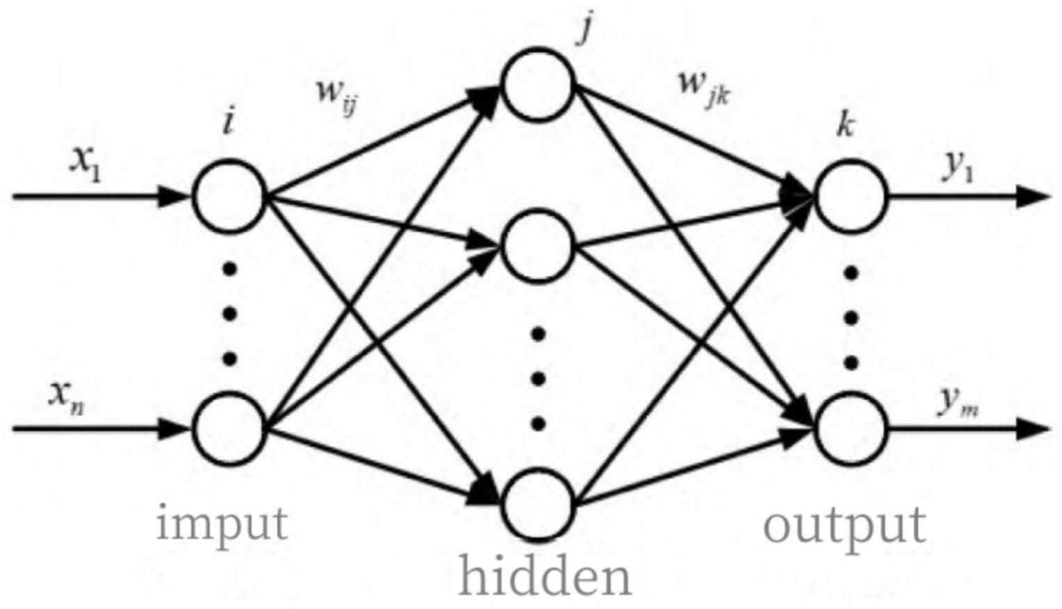
Figure 1. BP neural network structure.
Where(x1,x2,…,xm) denotes the input layer, Y = (y1,y2,…,ym) denotes the output layer, J = (j1,j2,…,jm) represents the implicit layer. wij andwjk represent the connection weights.
Referring to Liang (2022), the BP neural network modeling process is as follows.
(1) Signal forward propagation process
First, the Sigmoid function is set as the network activation function.
The input to the a node of the implicit layer neta is.
Where wij,δa are the weights of the hidden layer and the threshold of the a node, respectively.
The output of the a node of the implicit layer J is.
The input of the b node of the output layer netb is
where wij,δb are the weights of the hidden layer and the threshold value of the b node, respectively.
The output of the b node of the implicit layer Y is.
Where f is the Sigmoid activation function, and the symmetric Sigmoid function is chosen according to the characteristics.
(2) Error back propagation process
Set the learning rate as η, the error is calculated as follows.
The output layer weights are amended as follows
The error signal in the final output layer is obtained by deriving Equation 15 as
The output layer weights are adjusted as follows
The implied layer weight correction is expressed as
By deriving Equation 14 and calculating the error signal for the hidden layer via the chain rule as
And the implied layer weight adjustment results in
In the process of constructing a BP neural network, it is crucial to specify the number of nodes contained in the hidden layer, so this paper will find the appropriate number of nodes using the following formula, which is expressed as follows.
where m represents the number of nodes contained in the hidden layer, n is the number of nodes in the input layer, and u is the number of nodes in the output layer. a is a constant in the range [1,10].
As BP neural networks are relatively simple and have the disadvantage of easily falling into minima, while GA-BP neural networks are not prone to falling into local optimum traps during the specific search process, this paper will use GA-BP neural networks to simulate the pricing of carbon prices. The specific sequence of the model is as follows: individual coding → initialising the population → determining the fitness function → genetic operations (selection, crossover, mutation) → obtaining a new population → iterative optimisation → decoding the optimal solution. Where individual coding: S = NM+ML+M+L, N is the number of nodes in the input layer, M is the number of nodes in the hidden layer, L is the number of nodes in the output layer; fitness function: FIT = 1/MSE, MSE is the neural network mean square error performance function. In addition, this paper uses MatlabR2022b to set the maximum number of times the neural network learns to 1,000, the learning rate is 0.1, and the training accuracy is 0.000001. Regarding the setting of the parameters of the genetic algorithm, this paper sets the number of individuals to 40, the maximum number of genetic generations to 10, the crossover probability to 0.7, and the variation probability to 0.1.
4. Empirical analysis
4.1. Variable selection and variable testing
This paper selects daily data from January 2018 to August 2022, excludes non-overlapping dates and missing parts. The RMB/USD mid-price is used as a proxy variable in the exchange rate market, mainly considering that China’s exchange rate policy has been pegged to the USD for a long period of time, that there is also a path of influence between exchange rate fluctuations and carbon prices, reflected in energy prices and economic activities, and that the USD is the main denomination currency in international trade. Interest rate regulation is one of the instruments used to pursue monetary policy, which can also have an impact on firm output and carbon emissions. Shen et al. (2022) argue that the LPR has only been adjusted six times since the introduction of the LPR reform in 2019, and therefore the more flexible and versatile short-term interbank lending rate operational indicator better reflects the direction of interest rate policy, and therefore the 7-day interbank lending rate is chosen to represent the interest rate market. As China’s pilot carbon trading market has only spot transactions and the national unified carbon trading market was established on 16 July 2021, there is less data available for analysis and the study is not representative. Yan et al. (2022) argues that among the regional carbon markets, Hubei’s carbon market has a large trading volume, with a share of about 70% of the country. In this paper, the daily closing price of the Hubei carbon market is chosen as a proxy variable for the Chinese carbon market. The above data are obtained from the WIND database.
Since the return series are generally not smooth, as confirmed by the smoothness test on the original variables, this paper obtains the existing return series by doing logarithmic first-order differencing on all the series left. In this paper, each market variable after first-order differencing is defined as CNY, IR, CM.
As seen from the JB and P values in Table 1, none of the variables obey a normal distribution; as seen from the skewness and kurtosis, each return series exhibits a clear spike with a thick tail. This shows that there are general characteristics of the financial time series for each variable. From the results in Table 2, the yield series are smooth and have ARCH effects, which are consistent with the modeling conditions of GARCH-type models. Since the low-order GARCH(1,1) can reflect the aggregation characteristics of the yields, the next step is to use DCC-GARCH(1,1) to study the dynamic correlation between the exchange rate and interest rate, respectively and the carbon price. The next step is to construct a DCC-GARCH(1,1) using STATA17 to study the dynamic correlation between the exchange rate and interest rate, respectively and the carbon price.
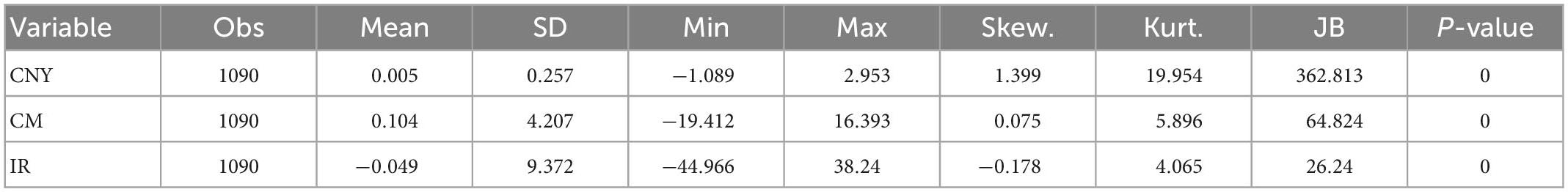
Table 1. Descriptive statistics.
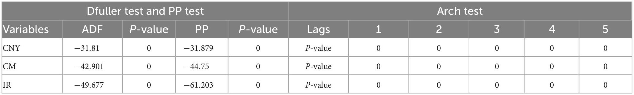
Table 2. Tests of stability and ARCH.
4.2. DCC-GARCH estimation
After constructing the DCC-GARCH, ARCH tests were performed on the residuals. From Table 3 it can be found that all have no ARCH effect at the 1% significance level, indicating that the model passes the test with a good fit and no heteroskedasticity. From the estimation results in Table 4, we can learn that in the equation, c represents the intercept term, a represents the ARCH term and b represents the GARCH term. All three are positive and significant at the 1% level, indicating that the GARCH model is reasonably reliable to set up. From the estimation results of the mean equation (x1), the AR(1) of carbon price and interest rate is negative, which means that the previous trading day has an inverse effect on the return of the current trading day, while the exchange rate market shows a positive effect. From the estimation results, the dynamic correlation coefficients are all positive; the result for Lambda1 indicates that the standardized residuals of the lagged period have a significant effect on the coefficients; the result for Lambda2 is close to 1, reflecting the long persistence of the dynamic correlation; the result for Lambda1+ Lambda2 is close to 1 indicating that the conditional covariance matrix is positive and satisfies mean reversion, further indicating that the DCC-GARCH model is robust and valid. Lambda1 reflects the short term adjustment in the conditional correlation coefficients between carbon prices and exchange rates and interest rates, while Lambda2 reflects the degree of long term adjustment. Lambda1 is 0.007 and Lambda2 is 0.981, which shows that the long term adjustment of carbon price and exchange rate and interest rate is significant, while the short term adjustment is relatively insignificant, indicating that exchange rate and interest rate will have a long term impact on carbon price, while the impact of shock is not significant in the short term.
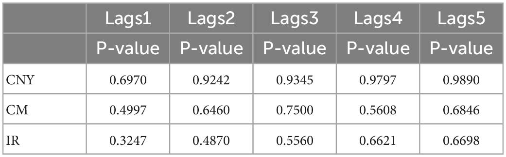
Table 3. ARCH test after modeling
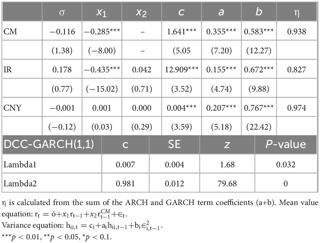
Table 4. DCC-GARCH estimation results.
| DCC-GARCH(1,1) | c | SE | z | P-value |
| Lambda1 | 0.007 | 0.004 | 1.68 | 0.032 |
| Lambda2 | 0.981 | 0.012 | 79.68 | 0 |
Figure 2 shows the dynamic correlation coefficients of the DCC-GARCH model. It is clear that the dynamic correlation coefficients between interest rates and carbon prices, and exchange rates and carbon prices, have time-varying characteristics and fluctuate more frequently and sharply.
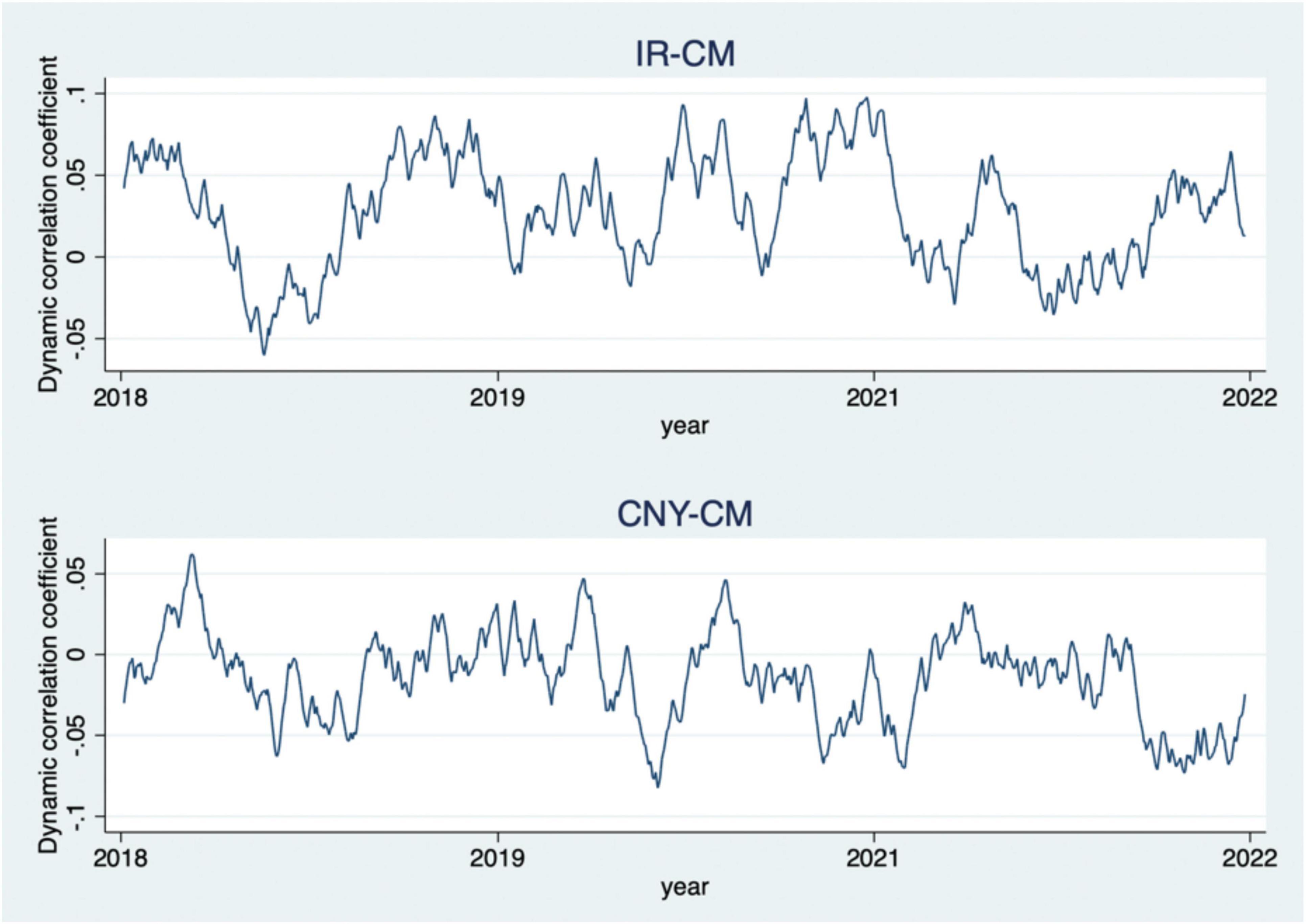
Figure 2. DCC coefficient diagram.
The dynamic correlation coefficient fluctuation range between exchange rate and carbon price is mainly concentrated in the [−0.08,0.07] interval. This is consistent with previous studies by scholars that there is a dynamic correlation between the exchange rate market and the carbon market, the logic of which is not repeated in this paper, please refer to the findings of Lu (2022) and Wang and Lu (2017, 2018) for more details. And this paper further builds on this result that fluctuations in interest rates also dynamically affect the direction of carbon prices. The dynamic correlation coefficient between interest rate and carbon price fluctuates mainly in the range of [−0.07,0.1], and the coefficient is mostly positive. Relatively stable and downward trending interest rates can reduce the cost of financing for companies. In mid-2018, interest rates had risen to a maximum value of 4.65%, which will greatly increase the cost of corporate financing, higher production and expansion costs, and lower carbon prices due to lower carbon demand. The dynamic correlation coefficient in Figure 2 falls to −0.07. After interest rates fall in 2020 and remain relatively stable thereafter, the dynamic correlation coefficient is mostly positive during this period.
4.3. TVP-VAR estimation
Wang and Zhao (2020) argues that VAR models focus on the inter-period correlation between variables and focus on causality. The use of VAR models would ignore the non-linear characteristics among markets, while TVP-VAR models compensate for this shortcoming. Therefore, in order to explore the transmission mechanism of exchange rates and interest rates on carbon prices, the TVP-VAR model is used instead of the VAR model in this paper. The descriptive statistics and smoothness tests of the variables prior to the construction of the TVP-VAR model have been described in the previous section and will not be repeated in this section.
From Table 5, the optimal lag order is 5. Therefore, referring to Nakajima (2011) model construction method, the nlag was set to 5 in MATLAB2022B. The number of MCMC samples was set to 10,000 and the first 1,000 samples were discarded to ensure the accuracy of the estimation results. The model estimation results are shown in Table 5 and Figure 2.
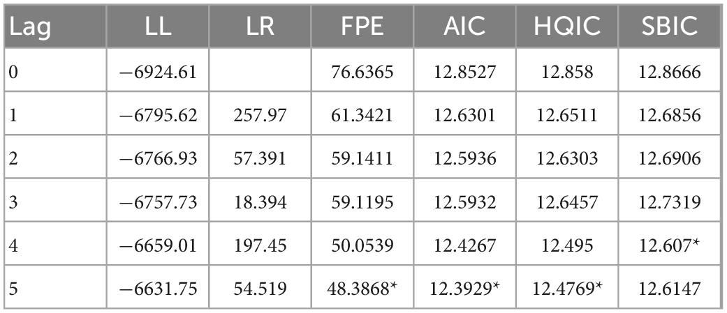
Table 5. Optimal lag order.
As seen in Table 6, the Geweke values are all significant at the 5% level, the hypothesis that the Markov chain converges to the posterior distribution is not rejected, and the null factor is generally low. As seen in Figure 3, the autocorrelation coefficient is decreasing; the path of values is relatively smooth; the graphical features resemble a normal distribution and the sampling is valid. Overall, the model estimates are valid, mutually independent and the fit is favorable.
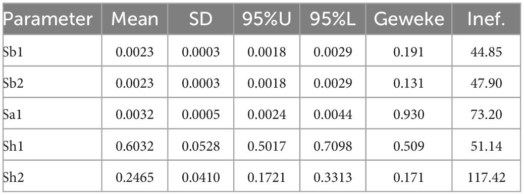
Table 6. Parameter estimation results.
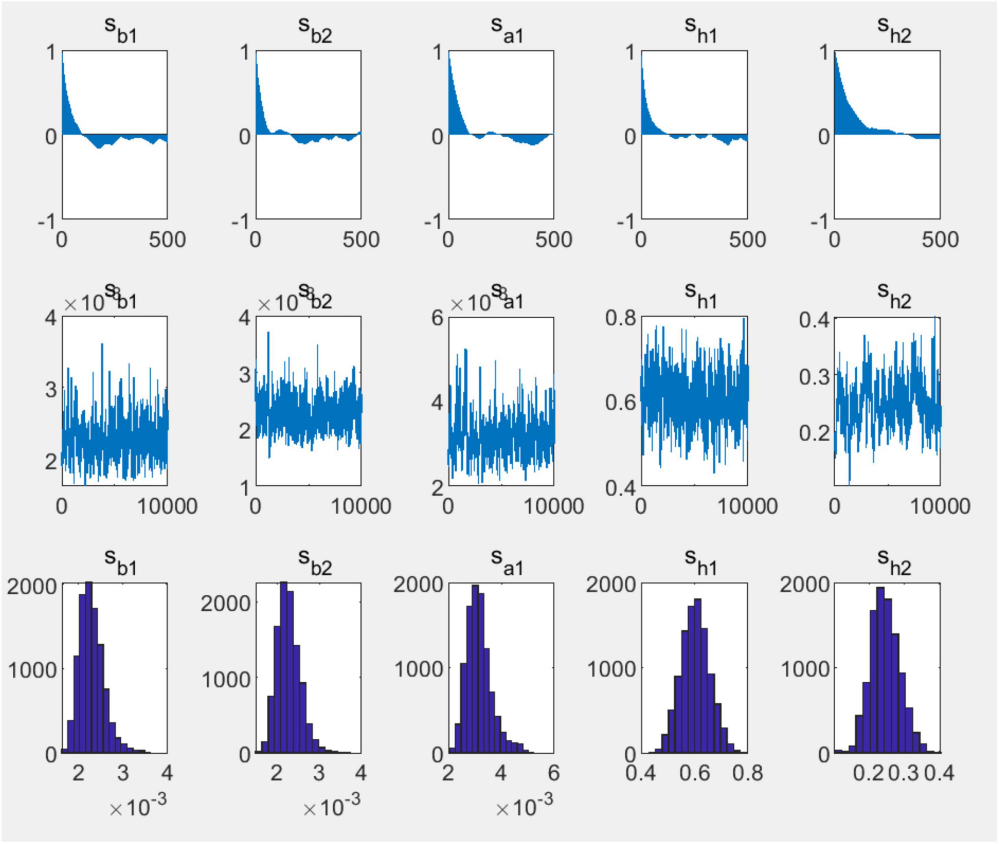
Figure 3. Parameter estimation results.
Figure 4 shows the time interval impulse response plots, with a lag of 1 month (short term), a lag of 6 months (medium term) and a lag of 12 months (long term) chosen in this paper to examine the response of carbon prices after 1 month, 6 months and 12 months when subjected to a positive shock of 1 unit of exchange rate and interest rate. The time-varying characteristics of the shock effects of exchange rates and interest rates on carbon prices are evident.
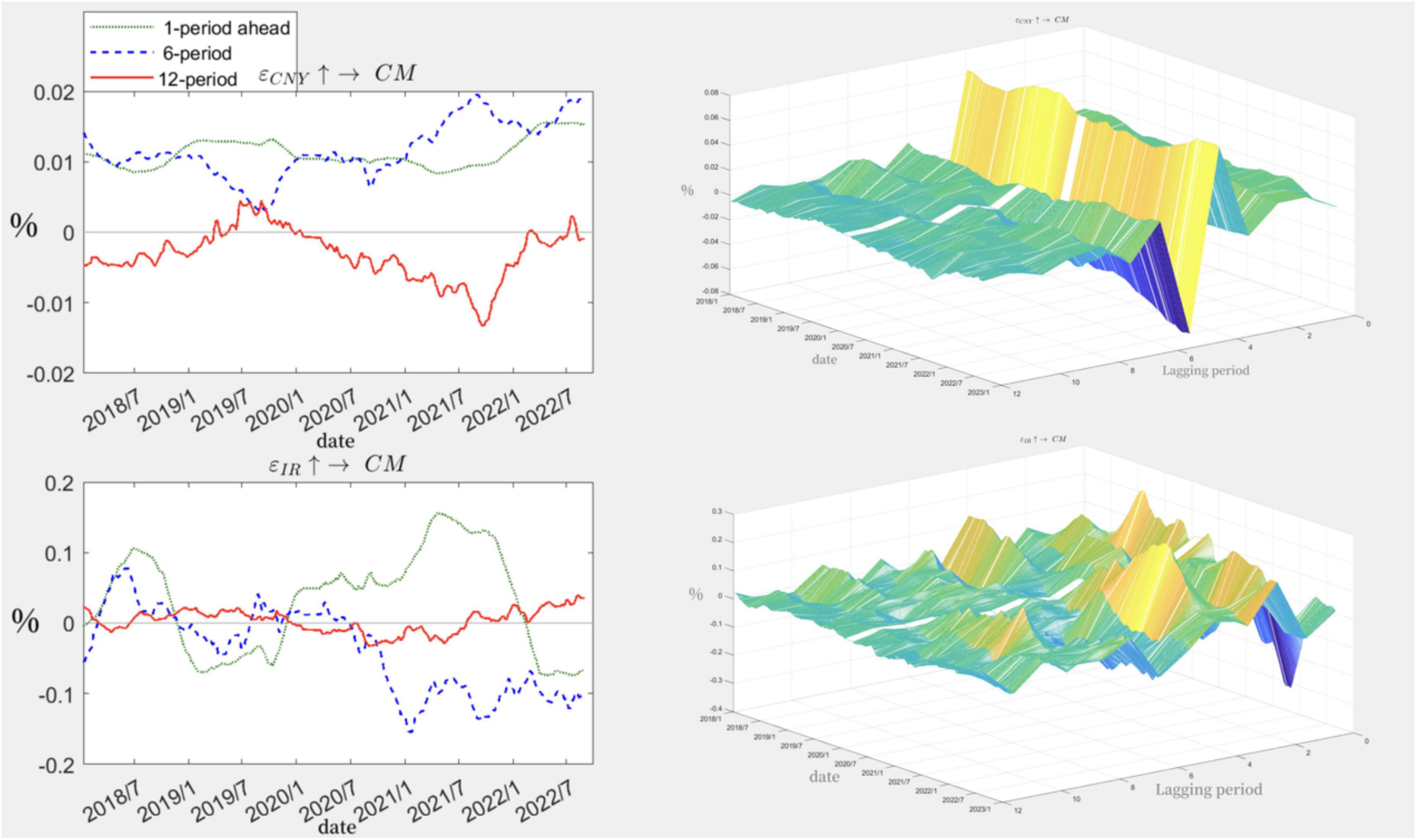
Figure 4. Equally spaced impulse response.
When carbon prices are subjected to exchange rate shocks, they are more affected in the short and medium term, and both are affected in a positive direction, but in the long term, the impact of exchange rates and interest rates on carbon prices diminishes and appears to be negative, but eventually the negative impact is gradually eliminated. When carbon prices are subjected to interest rate shocks, the short- and medium-term impulse responses are more consistent in the early part of the period, but over time they show opposite trends, and each is affected to a greater extent in both the positive and negative directions. In the long term, the impulse responses show a gradual weakening of the impact and a gradual stabilization of the carbon price. This is very different from the impact of an exchange rate shock. It can further be learned that when the exchange rate rises and the RMB depreciates, the carbon price rises in the short to medium term, which is consistent with the mechanism of the impact of exchange rate fluctuations on the carbon price described by Wang and Lu (2017). However, through the impulse response with a lag of 12 months, if the RMB continues to depreciate in the long run, it will lead to a decrease in carbon prices, which may be due to excessive currency depreciation, the gradual rise in energy import costs and the inability of enterprises to afford them, and the inability of energy substitution to be completed in the short term, leading to a decrease in profitability, a contraction in production, a decrease in demand for carbon emissions and a lower carbon price.
In addition, the impact of higher interest rates is not significant in the short term, but with the implementation of monetary policy, the price of carbon falls significantly in the medium term. The reason for this may be that the government authorities, in order to adjust the economy, reduce overcapacity or carry out environmental management, raise interest rates so that companies are less willing to produce products and increase production capacity, and the demand for carbon emissions decreases, thus leading to a gradual decrease in the price of carbon.
As can be seen from Figure 5, the three time points chosen for this paper are the operation of the China Science and Technology Board (June 2019), the release of the top-level design document for the “dual carbon” policy system (October 2021) and the Russia-Ukraine conflict (February 2022), all of which are the highest points for carbon prices in 2019, 2021 and 2022.
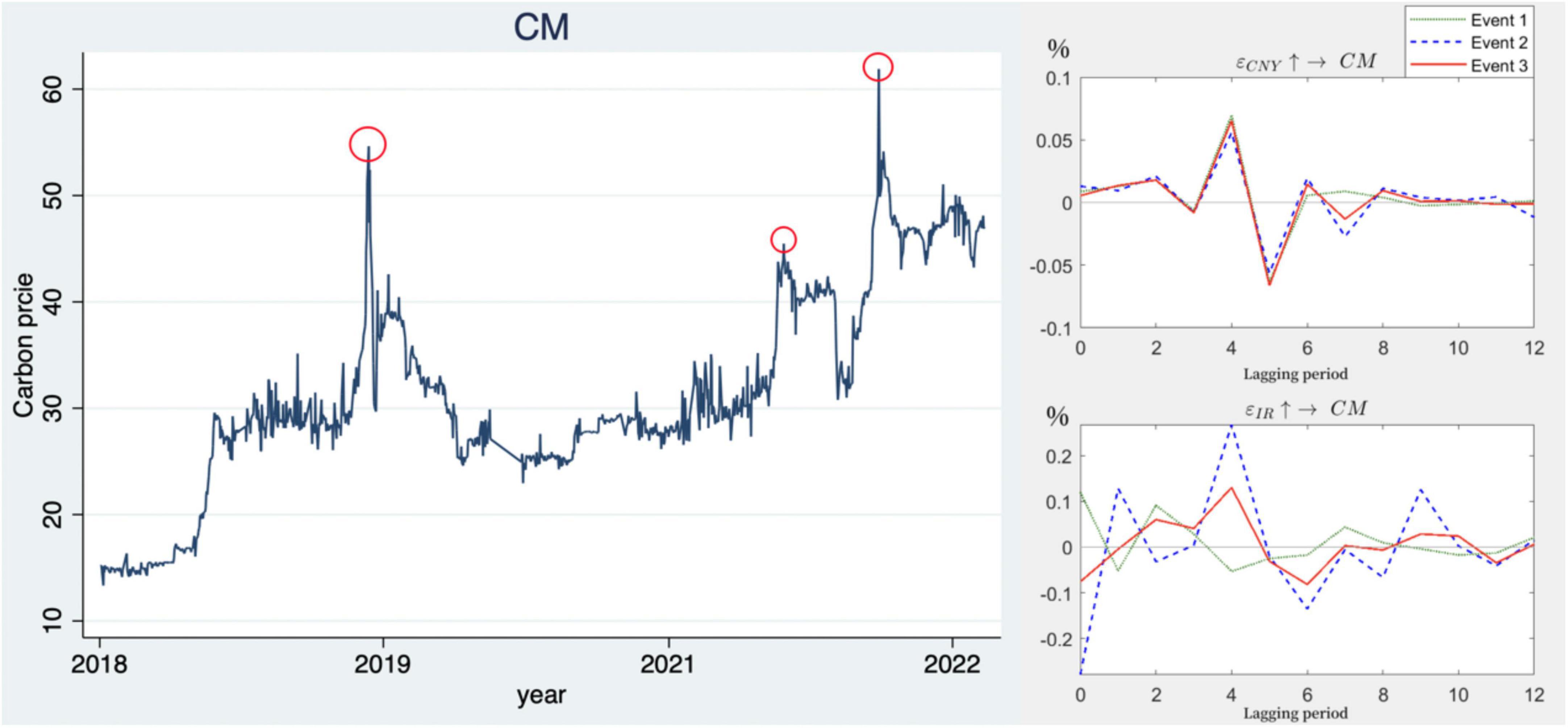
Figure 5. Impulse response at different points in time.
The impact of exchange rate shocks on carbon prices is roughly the same across the three time points, both reaching the maximum positive and maximum negative shocks at lag 4 and lag 5, respectively, and being relatively stable in the other lags. This shows that the RMB exchange rate is relatively robust under government regulation and is less affected by external transmission, similar to the iso-interval impulse response results, i.e., the negative impact of the exchange rate on the carbon price gradually disappears in the long run.
The effect of interest rate shocks on carbon prices varies between time points. At this point in the policy, the carbon price is most strongly affected by the interest rate shock, starting with a rapid response, with the positive shock effect reaching its peak in period 4, and then leveling off in period 10 after a period of volatility. The other two points in time also produced shocks that plateaued in period 10.
According to the empirical results of the TVP-VAR model, there are obvious time-varying characteristics between exchange rates, interest rates and carbon prices, with exchange rates and interest rates differing in positive and negative directions on carbon prices in the short, medium and long term. A sustained appreciation of the exchange rate will have a negative transmission to the carbon price, while adjustments in the interest rate in the short and medium term will have a dramatic impact on the carbon price, which adapts to the long-term changes in the interest rate before gradually stabilizing. The carbon market is more sensitive to interest rate effects than to exchange rate effects. External factors that influence interest rates can cause greater volatility in carbon prices, which can also be considered to be more sensitive to the impact of interest rates.
4.4. GA-BP neural network simulation analysis of carbon prices
Having determined that exchange rates and interest rates have a dynamic impact and transmission on carbon prices, in order to further predict the future trend of carbon prices after being influenced by both. In this paper, the carbon price is trained and simulated by using the exchange rate and interest rate as the input terms of the neural network and the carbon price as the output term. Three sets of 1,091 observations, all data were divided into a training and test set in the ratio of 8:2 and normalized. The simulation results presented in Figure 6 show that the model fits well overall and that the simulation analysis results derived from the model are reliable. The simulation results show that the error between the GA-BP neural network and the real value is very small, and the two have tended to overlap, which is obviously better than the simulation analysis of the BP neural network, in addition, the MSE of the GA-BP neural network is 0.027173, which shows that the use of the GA-BP neural network can improve the accuracy of the prediction of the carbon price and reduce the probability of error.
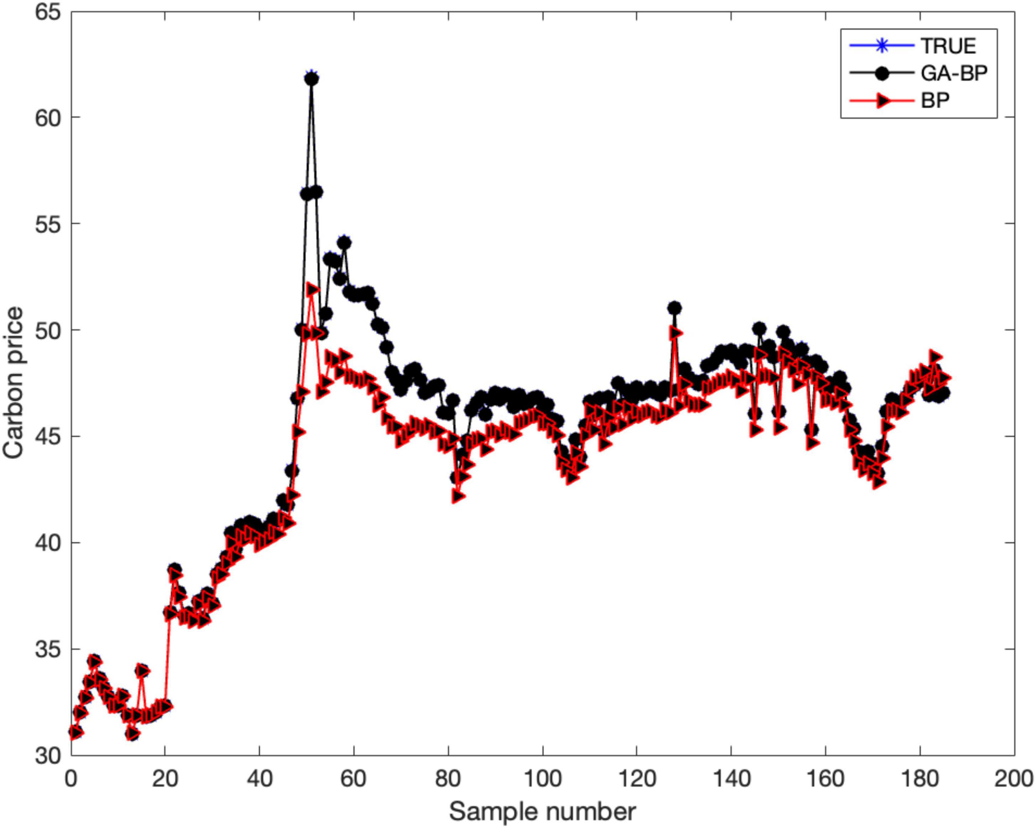
Figure 6. GA-BP neural network simulation results.
5. Conclusion and recommendations
Based on the empirical results, this paper draws the following conclusions: First, according to the dynamic correlation coefficient graph, it can be found that the interest rate is positively linked to the carbon price for most of the period from 2018 to 2022, while the exchange rate is more negatively linked to the carbon price. Secondly, the ‘exchange rate-carbon price’ is less affected by macro factors and external shocks, but the ‘interest rate-carbon price’ is, on the contrary, very sensitive to macro shocks. Thirdly, based on the training and simulation of the GA-BP neural network, the simulated and real values of the carbon price were found to be more consistent, suggesting that the movements of the carbon price simulated by machine learning can reflect the real situation to a certain extent. Carbon prices can fluctuate dramatically due to the combined effects of exchange rate and interest rate changes, which can provide an appropriate warning of future price fluctuations in carbon trading.
Based on the above empirical results, this paper gives the following recommendations: First, there is risk transmission from exchange rates and interest rates to the carbon market in the long, medium and short term. Keeping the exchange rate and interest rate stable, especially the interest rate, can reduce the transmission effect on the carbon price, avoid the surge or plunge caused by the shock, and ensure the smooth trading of the market. Secondly, the government needs to be cautious about the adjustment of exchange rates and interest rates, making appropriate adjustments to keep carbon prices stable and using market mechanisms to discipline the production activities of enterprises. Too low a carbon price will lead to an increase in energy consumption, which in turn will lead to an increase in carbon emissions. The government should build a mechanism to transform the green development of enterprises, pushing them to save energy and reduce emissions to achieve low-carbon transformational development. Thirdly, the government should not only introduce policies to support low-carbon enterprises, but also improve the national carbon market laws and regulations and price regulation mechanisms, and coordinate the policies of the regional carbon markets to avoid the occurrence of a systemic crisis in the carbon market affecting domestic industrial restructuring and the development of low-carbon industries.
Data availability statement
The original contributions presented in this study are included in the article/supplementary material, further inquiries can be directed to the corresponding author.
Author contributions
JY and YW contributed to conception and design of the study. JY organized the database, performed the statistical analysis, and wrote the first draft of the manuscript. YW and SS wrote sections of the manuscript. SS received the funding. All authors contributed to manuscript revision, read, and approved the submitted version.
Funding
This work was supported by General Project of National Social Science Foundation of China (21BJY251) and 2021 Scientific Research Capacity Improvement Project of Key Construction Subject of Department of Education of Guangdong Province (2021ZDJS37).
Conflict of interest
The authors declare that the research was conducted in the absence of any commercial or financial relationships that could be construed as a potential conflict of interest.
Publisher’s note
All claims expressed in this article are solely those of the authors and do not necessarily represent those of their affiliated organizations, or those of the publisher, the editors and the reviewers. Any product that may be evaluated in this article, or claim that may be made by its manufacturer, is not guaranteed or endorsed by the publisher.
References
Alberola, E., Chevallier, J., and Chèze, B. (2008). Price drivers and structural breaks in European carbon prices 2005-2007. Energy Policy 36, 787–797.
Bollerslev, T. (1986). Generalized autoregressive conditional heteroskedasticity. J. Econom. 31, 307–327.
Bollerslev, T., Engle, R. F., and Wooldridge, J. M. (1988). A capital asset pricing model with time-varying covariances. J. Polit. Econ. 96, 116–131.
Chai, S., and Zhou, P. (2018). The minimum-CVaR strategy with semi-parametric estimation in carbon market hedging problems. Energy Econ. 76, 64–75.
Chevallier, J. (2011). A model of carbon price interactions with macroeconomic and energy dynamics. Energy Econ. 33, 1295–1312.
Deng, J., Wang, Y., and Xuan, X. (2022). A study on the correlation between China’s carbon market and green bond market. Heat Power. 10, 61–71. doi: 10.19666/j.rlfd.202207130
Engle, R. F. (1982). Autoregressive conditional heteroscedasticity with estimates of the variance of United Kingdom inflation. Econ. J. Econ. Soc. 1982, 987–1007.
Han, J., and Jiang, Y. (2022). Study on the time-varying spillover effects of carbon market and non-ferrous metals futures market. Indust. Technol. Econ. 41, 113–123.
Liang, Q. (2022). Research on mushroom yield prediction method based on GA-BP neural network. Shandong: Shandong Agricultural University. doi: 10.27277/d.cnki.gsdnu.2022.000567
Lu, K. Y. (2022). Research on mushroom yield prediction method based on GA-BP neural network Ph. D., Thesis. Shandong Agricultural University.
Lv, J., Yang, H., and Guo, Z. (2020). A study on the effect of RMB exchange rate on carbon price shock in China by regions -based on VAR model. Price Monthly 6, 77–84. doi: 10.14076/j.issn.1006-2025.2019.06.12
Ma, M. J., Li, Q., Yin, W. Q., Zong, X., and Zhou, W. R. (2022). A GA-BP neural network-based carbon trading pricing model and its simulation under carbon neutrality target. Ecol. Econ. 3, 40–46.
Nakajima, J. (2011). Time-varying parameter VAR model with stochastic volatility: An overview of methodology and empirical applications. Monet. Econ. Stud. 29, 107–142.
Primiceri, G. E. (2005). Time varying structural vector autoregressions and monetary policy. Rev. Econ. Stud. 72, 821–852. doi: 10.1016/j.jpolmod.2020.03.014
Shen, S., Jiang, Z., and Liu, D. (2022). A study on the impact of the magnitude of interest rate regulation on financial markets. Price Theory Pract. 150–153+207. doi: 10.19851/j.cnki.CN11-1010/F.2022.05.218
Wang, Q., and Lu, J. (2017). Asymmetric effects of RMB exchange rate shocks on China’s carbon prices-an empirical study based on markov switching model. J. Soc. Sci. Jilin. Univ. 6, 95–206. doi: 10.15939/j.jujsse.2017.06.jj4
Wang, Q., and Lu, J. (2018). The shock effect of RMB exchange rate on carbon price in China-a perspective based on regional differences. J. Wuhan. Univ. 2, 157–165. doi: 10.14086/j.cnki.wujss.2018.02.016
Wang, S., and Zhao, C. C. (2020). Transmission mechanism between RMB exchange rate and stock prices-an empirical test based on DCC-GARCH model. Indust. Technol. Econ. 4, 54–62.
Yan, Z., Yu, Z., and Gu, X. (2022). A study on the transmission mechanism of carbon emission price and coal futures price in China. Econ. Issues. 6, 67–74. doi: 10.16011/j.cnki.jjwt.2022.06.008
Zhang, G., Wang, H., Hua, X., Liao, Y., and Peng, L. (2022). Study on the synergistic effect of foreign trade, technological progress and carbon emissions. Front. Ecol. Evolut. 718:971534. doi: 10.3389/fevo.2022.971534
Zhang, Z., and Chen, Y. (2015). Prediction of coal consumption and carbon emissions in China based on BP neural network. J. Hun. Univ. 1, 64–67. doi: 10.16339/j.cnki.hdxbskb.2015.01.009
Keywords: sustainable development, carbon price changes, exchange rates and interest rates, DCC-GARCH, TVP-VAR, GA-BP neural networks
Citation: Yang J, Wan Y and Shen S (2023) Research on the impact of exchange rates and interest rates on carbon price changes in the context of sustainable development. Front. Ecol. Evol. 10:1122582. doi: 10.3389/fevo.2022.1122582
Received: 13 December 2022; Accepted: 28 December 2022;
Published: 18 January 2023.
Edited by:
Praveen Kumar Donta, Vienna University of Technology, AustriaReviewed by:
Alaa Saleh, General Organization of Remote Sensing (GORS), SyriaChinnem Rama Mohan, Visvesvaraya Technological University, India
Mohd Asif Shah, Kebri Dehar University, Ethiopia
Copyright © 2023 Yang, Wan and Shen. This is an open-access article distributed under the terms of the Creative Commons Attribution License (CC BY). The use, distribution or reproduction in other forums is permitted, provided the original author(s) and the copyright owner(s) are credited and that the original publication in this journal is cited, in accordance with accepted academic practice. No use, distribution or reproduction is permitted which does not comply with these terms.
*Correspondence: Yuzhu Wan,  d2FueXV6aHUwNTE1QHpjc3QuZWR1LmNu