An improved Carnegie-Ames-Stanford Approach model for estimating ecological carbon sequestration in mountain vegetation

The vegetation in mountainous areas is abundant, and its ecological carbon sequestration ability is of great significance to maintain the sustainable and healthy development of the ecological environment. However, when estimating the carbon sequestration of mountain vegetation, the Carnegie-Ames-Stanford Approach (CASA) model assigns a uniform value to the maximum light energy utilization (ε_max = 0.389 gC/MJ), ignoring the influence of vegetation types and topographic factors on ε_max, resulting in the low accuracy of the CASA model in estimating the carbon sequestration of mountain vegetation. In this paper, the improved CASA model was combined with Landsat 8 Operational Land Imager (OLI) remote sensing image data to improve the estimation accuracy of carbon sequestration of mountain vegetation. The first was the establishment of a linear link between the terrain characteristics (slope and aspect), vegetation types, and ε_max in mountainous locations. The second was the improvement of the CASA model’s calculation method for key parameters. The different distributions of the estimation results from the two techniques in 2015 and 2016 are then compared using Landsat 8 data as the data source, and the impact of the terrain factors in the improved CASA model on the estimation results is confirmed. Finally, the improved CASA model and the CASA model are used to estimate the Net Primary Productivity (NPP) of the study area from 2000 to 2020, and the estimated results of the two models are compared with the computation results of the MODIS data NPP product. The findings indicate that the improved CASA model’s estimation results have a higher degree of fit and a better correlation. The improved CASA model aids in precisely understanding the ecological carbon sequestration potential of mountain areas and increases the estimation accuracy of vegetation carbon sequestration in mountainous areas.

Introduction

The CASA model primarily calculates NPP from light utilization efficiency (ε) and the Absorbed Photosynthetic Active Radiation (APAR) absorbed by vegetation. Although it is frequently used to estimate NPP (Field et al., 1998; Hicke et al., 2002; Singh et al., 2002; Xing et al., 2010), there are still some drawbacks. The calculation techniques for several parameters need to be updated because the original CASA model was built using NPP estimation of different types of vegetation in North America, which differs slightly from vegetation types in other countries (Yong et al., 2022). Second, when the same value of the maximum light use efficiency (ε_max) = 0.389 gC/MJ is assigned, the CASA model does not consider the impact of vegetation types on ε_max (Chen et al., 2017). Actually, different vegetation types have very varying ε_max (Chen et al., 2021). Additionally, the initial CASA model only established a functional relation with the Simple Ratio index (SR) for the Fraction of Absorbed Photosynthetically Active Radiation (FPAR), which was insufficient to identify the internal link between FPAR and vegetation. Last but not least, it is difficult to obtain the soil parameters required for CASA model estimation, with low accuracy and complex calculation, which can easily affect the estimation results (Wang H. et al., 2019; Zhu et al., 2019).

Mountainous vegetation is rich and diverse, and improving the estimation accuracy of the ecological carbon sequestration in mountainous areas can provide a clearer understanding of the ecological carbon sequestration capacity of mountain vegetation (Xu et al., 2020; Jiang et al., 2021; Li H. et al., 2021; Li Y. et al., 2021; Zhang et al., 2021). Wang et al. (2020) showed that from 2010 to 2016 in mainland China, the carbon sequestration of terrestrial ecosystems was 45% of the anthropogenic carbon emissions during the same period, approximately 1.11 billion tons, and these carbon sequestration contributions are mainly due to the strong ecological carbon sequestration capacity in the southwestern mountainous areas of China. The high slope and significant fluctuation of mountain areas, however, make it easy for topographic elements to alter the accuracy of the assessment of vegetation carbon sequestration (He et al., 2018; Yu et al., 2020; Li M. et al., 2021; Li Y. et al., 2021; Li et al., 2022; Wang et al., 2022). The Surface Water Sub-Index was used to enhance the parameters in the CASA model, which decreased the influence of terrain elements on estimation accuracy (Pan and Xu, 2020; Xia et al., 2020). The precision of the data they used, however, had a significant impact on the estimation outcomes. To lessen the influence of topographic factors on the estimation of vegetation carbon sequestration, Chen and Sun et al. introduced the Shadow Elimination Vegetation Index (SEVI) into the model (Chen and Zeng, 2016; Sun and Xie, 2021). However, this method was difficult to use to eliminate the impact of shadows on slopes with large slopes. To some extent, Geng et al. revised the CASA model’s parameters based on the Digital Elevation Model (DEM) data to increase the estimation accuracy of the CASA (Wang H. et al., 2019; Wang Y. et al., 2019), but this method’s correcting effect on terrain falling shadow is subpar. Early studies have shown (Sun et al., 2016; Li H. et al., 2021) that changing model parameters is challenging when assessing vegetation carbon sequestration at a wide range of regional scales. They only established the value range of ε_max based on experimental data but did not establish a functional relation between terrain parameters and the ε_max (Han, 2020; Peng et al., 2021). Therefore, the estimation results of the improved model are significantly different from those of previous methods (Liu Y. et al., 2013; Fan, 2018; Jiang et al., 2019; He et al., 2019; Li et al., 2019a,b).

The primary goals of this paper, which are based on the aforementioned issues, are to (1) address the issue that the CASA model’s ε_max is uniformly set at 0.389 g C/MJ and (2) establish a functional relationship between ε_max and vegetation types and terrain factors so that ε_max changes as the terrain changes; then, (3) lessen the effect of topographic factors on the accuracy of vegetation carbon sequestration estimates in mountainous areas and establish a functional relationship between topographic factors and vegetation NPP in conjunction with the fact that vegetation resources are primarily distributed in mountainous areas with high relief (Shen et al., 2022; Zhao et al., 2022). As a result, this paper estimates the NPP value of the study area using the improved CASA model based on Landsat 8 OLI data sources in Sichuan mountainous areas, analyses the relationship between the estimated results in different periods in the same area and the topographic factors, and confirmes the viability of the improved CASA model. Then, the correlation and the fitting degree of the estimation results of the three methods (CASA model, improved CASA model, and MODIS data NPP product) are compared to verify whether the estimation accuracy of the improved CASA model has been improved.

Materials and methods

Study area

The study area should have a mountainous distribution to meet the research objectives. Second, the research region should also have a reasonably flat area distribution to more clearly discern the differences in vegetation estimating findings between the two models for various terrain features. As a result, this article uses some of the neighboring Sichuan mountain areas and Chengdu Plain as its research area and chooses high-quality Landsat 8 OLI data from the geospatial data cloud as its data source. According to previous research results on mountain areas in China (Christian and Jens, 2011; Zhang et al., 2013, 2022; Price et al., 2019; Körner et al., 2021; Zhang and Min, 2022), the selected definition criteria for Sichuan mountain areas are as follows: areas with elevations less than 500m and degrees of relief greater than 50m; elevations between 500 and 2500 m, degrees of relief higher than 100 m or slopes greater than 25^°; and elevations greater than 2500 m. According to GIS calculations, the Sichuan mountainous areas is 328,500 square kilometers, and the plain and hilly area is 157,500 square kilometers. The distribution range of mountainous areas and the spatial location of Landsat 8 OLI image data required in this paper are shown in Figure 1.

FIGURE 1

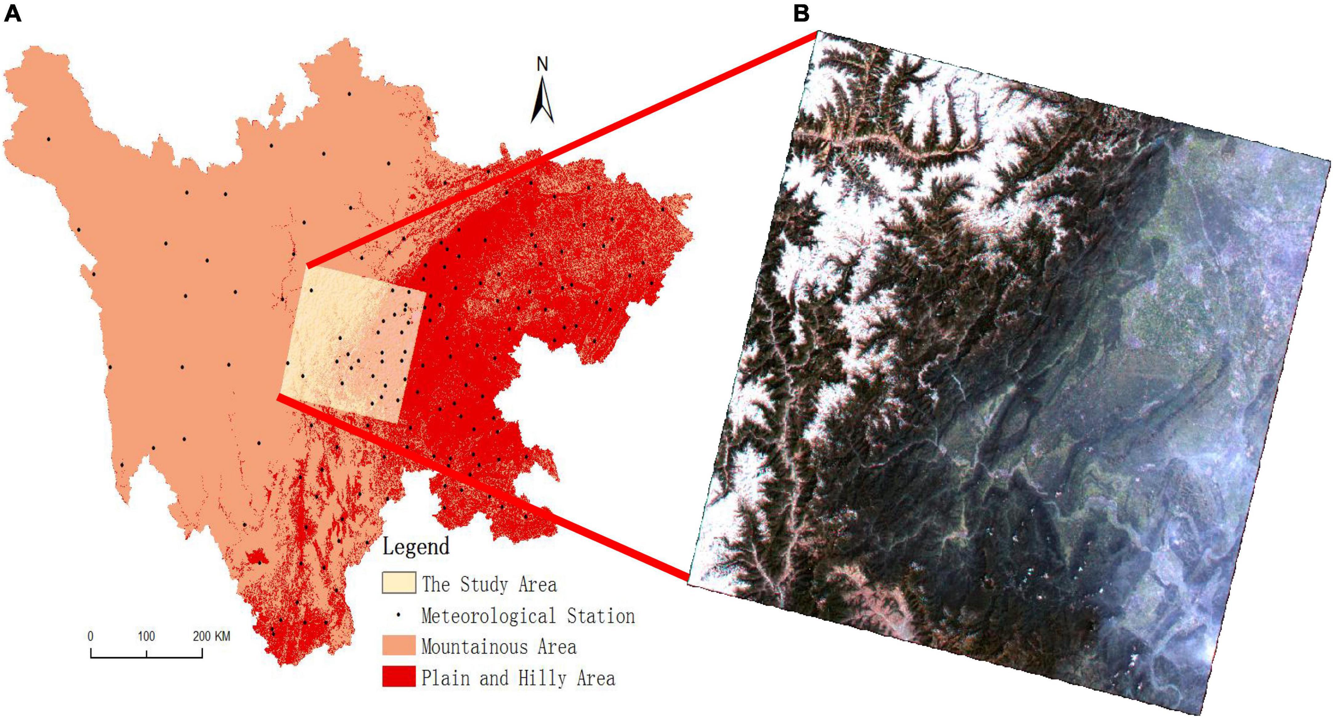
Figure 1. Distribution of the study area and meteorological stations in the Sichuan mountainous areas (A) and Landsat 8 OLI data image in the study area in June 2016 (B).

The study area is high in the northwest and low in the southeast, with relatively low elevation in the east and large topographic relief. The west and north have relatively high elevations and relatively flat terrain. Affected by topographic factors, the eastern and southern parts of the study area have more precipitation and higher temperatures, while the western and northern parts of the study area have less precipitation and lower temperature. Therefore, forests, shrubs, and other vegetation are mainly distributed in the east and south of the study area, with rich and diverse vegetation types, while grasslands, shrubs, and other vegetation are mainly distributed in the west and north, with a single vegetation type.

Data and processing

Landsat 8 operational land imager data

Remote sensing data are mainly used to calculate vegetation parameters involved in the model. The remote sensing data required in this paper are Landsat 8 OLI data with good quality in the second quarter of each year from 2000 to 2020, including data information from 11 bands. All Landsat 8 OLI data are downloaded from the geospatial data cloud.¹ Before data processing, radiometric correction, atmospheric correction, and other preliminary processing work are needed. Then, band 4 and band 5 in the data were used for function calculation to calculate the vegetation index required by the paper, such as the Normalized Difference Vegetation Index (NDVI), the Simple Ratio Index (SR), the Leaf Area Index (LAI), and so on.

Digital elevation model

The DEM data required by the paper are from the geospatial data cloud, (see text footnote 1) with a spatial resolution of 90 m. DEM data are mainly used to calculate the spatial distribution, slope, aspect, and other information of mountain areas. The DEM data of Sichuan mountainous areas are obtained by clipping the mountain areas based on the DEM data of Sichuan Province.

MOD17A3HGF data product

The NPP product data required in this paper are used to verify the accuracy of the improved CASA model and the estimated results of the CASA model for carbon sequestration. Based on the MOD17A3HGF dataset, the MODIS MOD17A3HGF NPP data of the study area from 2000 to 2020 were generated through the processing of splicing, projection transformation and cropping of the segmentation images covering the study area. This dataset has a spatial resolution of 500 m and a temporal resolution of 8 days.

Meteorological data

Meteorological data are mainly used to calculate the climate parameters involved in the model. The average daily temperature, hours of sunshine, and daily precipitation used herein were provided by the National Meteorological Information Center² (National Meteorological Information Center [NMC], 2018). The paper selects 156 meteorological station data in Sichuan Province (as shown in Figure 1), interpolates the meteorological data in Sichuan Province using the Inverse Distance Weight method (IDW) of ARCGIS software, and then uses the mask data in the mountain area to cut them, thus obtaining the meteorological data in Sichuan mountain areas. As seen from Figure 1, meteorological stations are distributed less in the west and more in the east, and the overall distribution is relatively uniform, which is conducive to the accurate acquisition of meteorological data. The processing consisted of the following sections:

(1) Meteorological data from meteorological stations around the research area were selected to obtain monthly average temperature, total sunshine hours and total precipitation.

(2) Assign the spatial coordinate information based on the longitude and latitude of each station to the meteorological data.

(3) Meteorological data with a spatial resolution of 90 m are obtained by the IDW interpolation method of meteorological station data.

Vegetation types data

Vegetation types data are used to determine ε_max of different vegetation, and ε varies greatly with different vegetation types. Papers required for vegetation types data from the resources and environmental science data center of the Chinese Academy of Sciences.³ According to the data on vegetation distribution in Sichuan mountainous areas, ε_max among different vegetation types can be calculated.

Improvement of Carnegie-Ames-Stanford Approach model

The CASA model is one of the most representative sunshine energy utilization models (Du et al., 2021) and it is not solely easy in structure and high in responsiveness; however conjointly widely utilized in vegetation NPP estimation on giant spatial and international scales (Cai et al., 2018; Yang, 2019). To date, it is a comparatively mature calculation method that incorporates a certain theoretical basis, the parameters are straightforward to obtain (Chen et al., 2021), and the calculable NPP accuracy is high (Li et al., 2019a; Liu et al., 2020; Zhang et al., 2020). The CASA model calculates NPP through two variables: APAR and ε. Therefore, this paper mainly improves their calculation methods.

Improvement of ε

The calculation method of ε according to the CASA model is shown in Formula 1(Du et al., 2021), most parameters square measure the typical air temperature (T_ε1 and T_ε2) and the average evaporation (W_ε). However, because of the massive fluctuation of the piece of ground within the study space, the temperature distinction between the highest and bottom of the slope is giant, and the evaporation is completely different.

${\mathrm{\epsilon = \epsilon }}_{\text{max}}*{\text{T}}_{\text{ε}1}*{\text{T}}_{\text{ε}2}*{\text{W}}_{\text{ε}}(1)$

In the formula, ε_max represents the highest utilization rate of sunshine energy (gC/MJ), and T_ε1, T_ε2, and W_ε represent the parameters of ε_max at vasoconstrictor, heat, and water stress, respectively.

This research improves the calculation method of ε by merging it with other carbon sequestration estimating models (Vegetation Photosynthesis Model, VPM; Vertically Generalized Productivity Model, VGPM, etc.) to increase the estimation accuracy of the CASA model in mountainous areas. To lessen the influence of terrain characteristics on the estimation accuracy, the parameters involved in ε are obtained using band reflectance as much as feasible. The improved equation is:

${\mathrm{\epsilon = \epsilon }}_{\max }*{\text{ Tem }}_{}*\mathrm{ Wat }(2)$

In the formula, ε_max represents the maximum light energy utilization (gC/MJ), Tem is the temperature parameter and Wat is the vegetation leaf age and water content parameter.

The improvement of ε_max

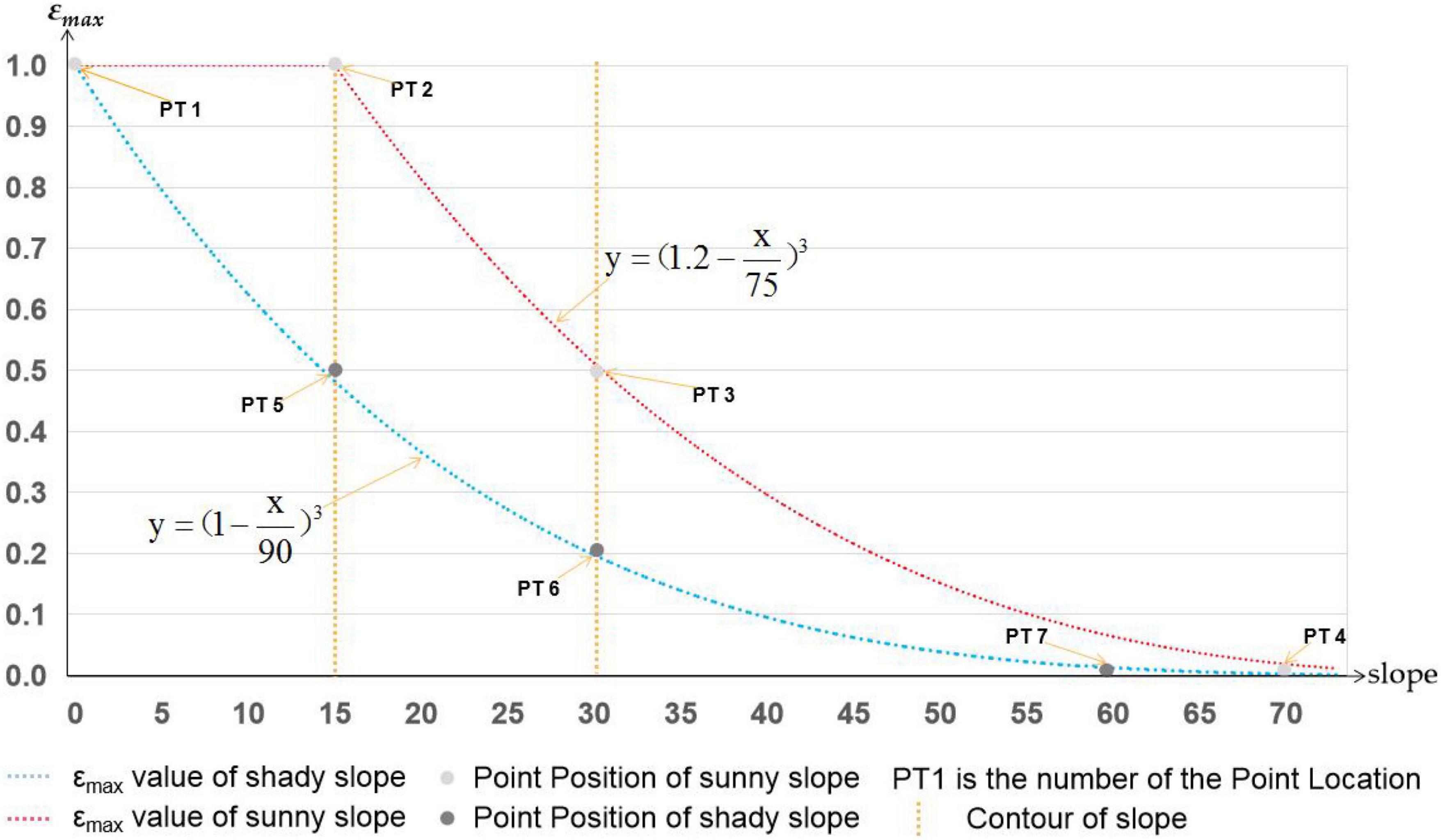
According to previous research results, the size of ε_max depends on vegetation types, NDVI and LAI, and their geometric relationship (Equation 3) is established (Anikó et al., 2017). However, the effect of topographic factors on ε_max is ignored. Therefore, based on previous studies, this paper added topographic factors (slope and aspect) into the geometric relationship and constructed the functional relationship between ε_max and slope, aspect, vegetation types, NDVI, and LAI (Equations 3–5). To build a functional relationship between terrain factors and ε_max, first, the point information of at least 3 points location (PT) should be determined in the same coordinate system (slope as abscissa, ε_max as vertical coordinate). ε_max on sunny and shady slopes fluctuates depending on the angle of irradiation and the area of light received under the same sunshine due to the influence of slope and aspect (Li Y. et al., 2021). For plants on the sunny slope, when the slope is small, ε_max does not change much (PT 1) (Zhang and Ren, 2016). When the slope is larger than 15°, ε_max will decline exponentially as the slope rises (PT 2) (Xu et al., 2019); at 30°, ε_max is only 0.5 times the slope’s bottom (PT 3) (Li H. et al., 2021; Li M. et al., 2021); and until the slope is approximately 70°, ε_max is essentially zero (PT 4). The reason is that when the slope increases, the soil water content and thickness decrease due to the effects of gravity, which has a direct impact on how well flora use solar energy (Sun et al., 2014; Wang B. et al., 2021; Wang J. et al., 2021). For vegetation on shady slopes, ε_max decreases with the increasing slope (Zhang et al., 2021). When the slope increases to 15°, ε_max is only half of the slope bottom (PT 5) (Zhu and Yuan, 2019), and when the slope increases to 30°, ε_max is only 0.2 times the slope bottom (PT 6) (Du et al., 2018). When the slope increases to 60° (PT 7), ε_max is 0 (Zhang et al., 2020). The reason is that with the increase in slope, the soil thickness and water content decrease, while the shielding areas between vegetation increase, which reduces the illumination areas of shady slope vegetation, resulting in ε_max decreasing gradually (Zhu et al., 2006; Li et al., 2022). According to the rules summarized by predecessors above, for the functional relationship between the two in a sunny slope area, the formula y = (1.2-x/75)³ can well couple the relationship between the two. For the shady slope area, the formula y = (1-x/90)³ is found to be able to couple the relationships. Therefore, these two formulas were put into Equation 3 to establish the functional relationship between the slope aspect and ε_max (Equations 4 and 5). However, this is only an ideal function. ε_max is also affected by vegetation types, the spatial distribution of vegetation types is affected by altitude, and the vegetation types change regularly with altitude. According to the above analysis, the relationship between ε_max and slope and facet is shown in Figure 2, and the value of ε_max is not fixed but changes with the change in slope and aspect.

FIGURE 2

Figure 2. The relationship between slope, aspect and ε_max.

To estimate the carbon sequestration of mountain vegetation more accurately, it is necessary to establish the geometric relationship between ε_max and slope and aspect. According to previous studies, ε_max varies greatly with different vegetation types, and its size depends on vegetation types, NDVI, and LAI (Yang et al., 2015; Yan et al., 2022). In this paper, the slope and aspect are taken as the influence parameters to improve the previous calculation method of ε_max. The improved calculation method of ε_max is:

The calculation equation of ε_max of sunny slope vegetation is:

${\mathrm{\epsilon }}_{\text{max}}={\text{k}}_1*{\text{a}}_{\text{max}}^{\text{n}}+{\text{k}}_2*\text{NDVI}*\mathrm{LAI},0\le \text{S}\le 15,\mathrm{ }\text{n}=1,2,3\mathrm{\dots }(3)$

${\mathrm{\epsilon }}_{\text{max}}={\text{k}}_1*{\text{a}}_{\text{max}}^{\text{n}}*{\left(1.2-\frac{\text{x}}{75}\right)}^3+$

$\mathrm{\hspace{1em}\hspace{1em}\hspace{1em}\hspace{1em}\hspace{1em}\hspace{1em}\hspace{1em}\hspace{1em}\hspace{1em}\hspace{1em}\hspace{1em}}{\text{k}}_2*\text{NDVI}*\mathrm{LAI},\mathrm{S}>15,\mathrm{n}=1,2,3\mathrm{\dots }(4)$

The calculation formula of ε_max for shady slope vegetation is:

${\mathrm{\epsilon }}_{\text{max}}={\text{k}}_1*{\text{a}}_{\text{max}}^{\text{n}}*{\left(1-\frac{\text{x}}{90}\right)}^3+$

$\mathrm{\hspace{1em}\hspace{1em}\hspace{1em}\hspace{1em}\hspace{1em}\hspace{1em}\hspace{1em}\hspace{1em}\hspace{1em}\hspace{1em}\hspace{1em}}{\text{k}}_2*\text{NDVI}*\mathrm{LAI},\mathrm{S}>0,\mathrm{n}=1,2,3\mathrm{\dots }(5)$

In the formula, aⁿ_max is the maximum value of light energy utilization efficiency of the same vegetation; S is the slope, taking a positive integer; and n is the species and quantity of vegetation. k is the adjustment coefficient. When NDVI ≤ 0.1, k₁ = 0, k₂ = 0; when NDVI > 0.1, k₁ = 1, k₂ = 0.1.

According to the vegetation distribution data in Sichuan mountain areas, the spatial distribution of different types of mountain vegetation can be obtained, and ε_max of different types of mountain vegetation in Sichuan can be obtained by referring to previous studies (Table 1) (Zhu et al., 2006; Wang B. et al., 2013, Cai et al., 2014; Wang et al., 2015; Du et al., 2017; Tang et al., 2017; Lan et al., 2018).

TABLE 1

Table 1. ε_max of different vegetation types in the study area under ideal conditions.

The ε_max value of different vegetation will change according to the external conditions (Zhu et al., 2006; Li et al., 2012). The functional relationship between ε_max and slope and aspect was established according to Equations 3–5 (Figure 2). On this basis, according to Landsat 8 data (Figure 3B), the spatial distribution of hillside vegetation types and the relationship between altitude (Figure 3A) and ε_max values of different vegetation types (Table 1), the functional relation between ε_max values of different vegetation types and slope (Figure 3C) was calculated through Equations 3–5. In Figure 3A, the vegetation types are divided into seven categories from low to high altitude, and their ε_max values under ideal conditions are shown in Table 1. According to the slope size and slope orientation, only suitable equations are selected from Equations 3–5 to calculate ε_max. The calculation results are shown in c in Figure 3. The uniform value of ε_max of the CASA model is 0.389 (gC/MJ), while ε_max of the improved CASA model changes with the change in vegetation types, slope, and aspect. This characteristic of the improved CASA model is more consistent with the actual situation of vegetation ε_max. When the sunny slope is less than 35° or the shaded slope is less than 30°, the ε_max value of the improved CASA model is larger than that of the CASA model. In this paper, Equations 3–5, and ε_max in the ideal state of vegetation in Table 1 are used to establish the functional relation between the ε_max value of mountain vegetation and vegetation types, slope, and aspect.

FIGURE 3

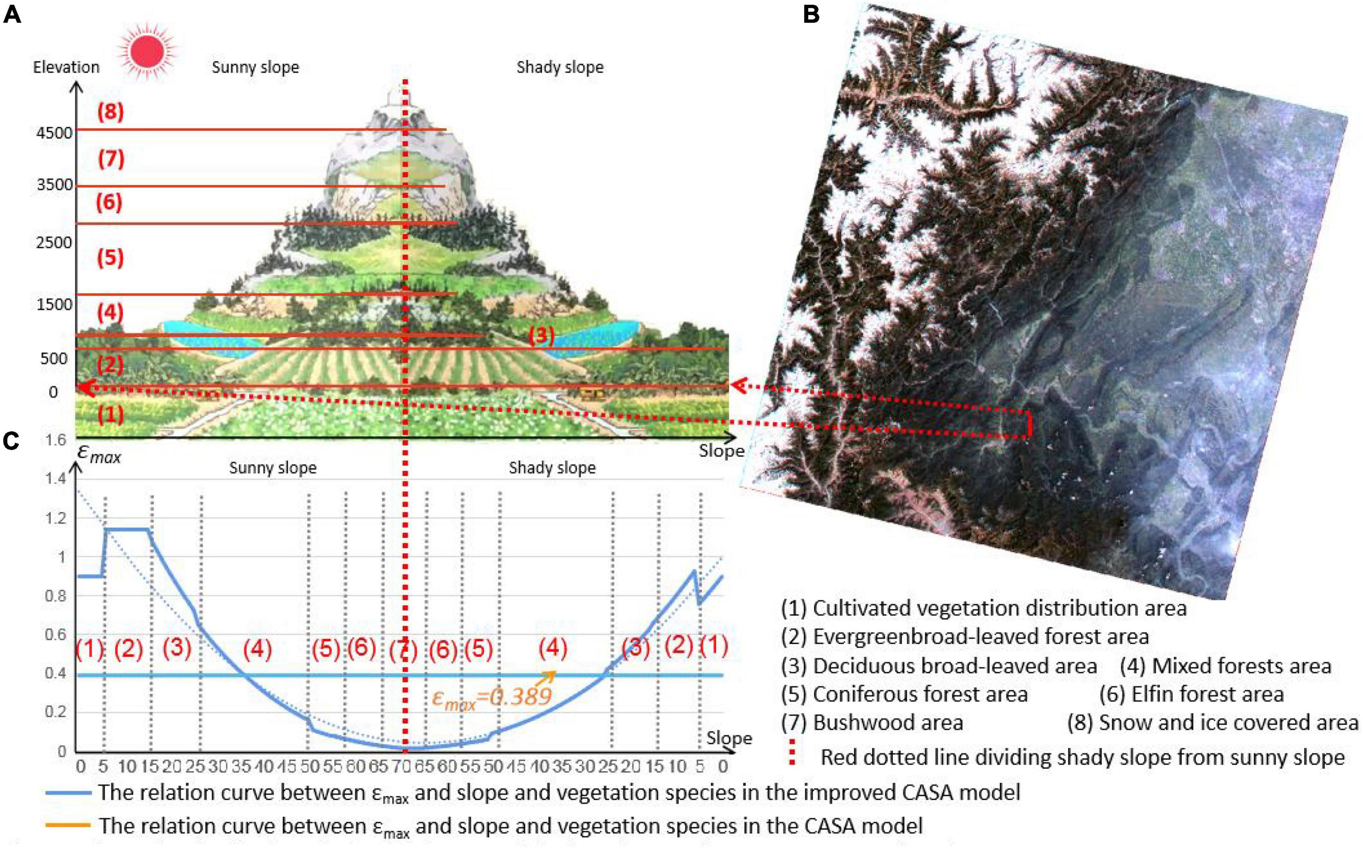
Figure 3. Relationship between the ε_max value and slope, aspect, and vegetation types in the improved CASA model and the CASA model. (A) Shows the distribution relationship between altitude and vegetation type. (B) Is the position of figure a in the remote sensing image. (C) The blue line is the distribution curve of e calculated with the change of vegetation type, slope and aspect in the improved CASA model, while the yellow line is fixed value of e determined with the change of vegetation type, slope and aspect in the original.

The improvement of tem

Tem indicates the stress parameter of the external temperature on light energy utilization. Its calculation formula is (Wang Y. et al., 2019):

$\text{Tem}=\frac{\left(\mathrm{T}-{\text{T}}_{\text{min}}\right)\left(\mathrm{T}-{\text{T}}_{\text{max}}\right)}{\left(\mathrm{T}-{\text{T}}_{\text{min}}\right)\left(\mathrm{T}-{\text{T}}_{\text{max}}\right)-{\left(\mathrm{T}-{\text{T}}_{\text{opt}}\right)}^2}(6)$

T_min, T_max, and T_opt are also known as the three fundamental temperatures, which are the lowest, highest and best temperatures of vegetation during photosynthesis. The three fundamental temperatures of different vegetation types are usually obtained by a literature collection (Chen et al., 2014). After consulting relevant documents (Peng et al., 2000; Zhang et al., 2012, 2014; Li, 2013; Wang L. et al., 2013), the three base temperatures of the main vegetation in the study area are shown in Table 2.

TABLE 2

Table 2. Three benchmark temperatures for the main vegetation in the study area.

The improvement of wat

Wat is the product of vegetation leaf age and leaf water content parameters, indicating the impact of vegetation leaf age and water content on light energy utilization. The calculation formula of Wat is (Zhang and Zhang, 2017; Yan et al., 2018):

$Wat=\frac{{\left(1+\text{LSWI}\right)}^2}{2\left(1+{\text{LSWI}}_{\text{max}}\right)},\text{LSWI}=\frac{\text{(NIR}-\text{SWIR)}}{\text{(NIR}+\text{SWIR)}}(7)$

In the formula, NIR represents the reflectance of vegetation in the near-infrared band, and SWIR represents the reflectance of vegetation in the infrared band.

Improvement of absorbed photosynthetic active radiation

In this paper, the calculation method of APAR is improved, and the improvement of the calculation method of APAR is mainly the improvement of FPAR (Zhu et al., 2019). In the CASA model, the functional relationship between the FPAR and SR index (Equation 9) is used to calculate the FPAR. However, according to the research findings, the calculated results of FPAR based on SR are usually lower than the measured values because the NDVI index is inconsistent with the measured values due to the shadow caused by the ground potential factor (Chen et al., 2018; Wang H. et al., 2019; Wang et al., 2020; Xia et al., 2020). Therefore, in the calculation of FPAR, instead of using the CASA model to calculate the formula of FPAR, the paper selected the average value of the calculated results (Equation 12) of the SR index, EVI index, and NDVI (Equations 9–11) that had a functional relationship with FPAR as the final FPAR value (Li H. et al., 2021; Li M. et al., 2021; Li Y. et al., 2021).

$\text{APAR}=\text{SOL}*\text{FPAR}*0.5(8)$

${\text{FPAR}}_{\text{SR}}=\text{min}(\frac{\text{SR}-{\text{SR}}_{\text{min}}}{{\text{SR}}_{\text{max}}-{\text{SR}}_{\text{min}}},0.95),\text{SR}=\frac{\text{NIR}}{\text{R}}(9)$

${\text{FPAR}}_{\text{EVI}}=\text{a}*\mathrm{ }\text{EVI}(10)$

${\text{FPAR}}_{\text{NDVI}}=\frac{\left(\text{NDVI}-{\text{NDVI}}_{\text{min}}\right)\left({\text{FPAR}}_{\text{max}}-{\text{FPAR}}_{\text{min}}\right)}{\left({\text{NDVI}}_{\text{max}}-{\text{NDVI}}_{\text{min}}\right)}+{\text{FPAR}}_{\text{min}}(11)$

$\text{FPAR}=\frac{\left({\text{FPAR}}_{\text{SR}}+{\text{FPAR}}_{\text{NDVI}}+{\text{FPAR}}_{\text{EVI}}\right)}{3}(12)$

In the formula, a is the empirical coefficient, FPAR_max and FPAR_min are the maximum and minimum values of FPAR, and the values taken as are 0.95 and 0.001.

Validation of the model

To verify the feasibility of estimating vegetation carbon sequestration by the improved CASA model, it is necessary to verify the spatial relationship between slope, slope aspect, and the difference in estimating carbon sequestration by the two models (the improved CASA model and the CASA model).

Verification of slope

In this paper, the improved CASA model and CASA model are used to estimate the vegetation NPP of Landsat 8 OLI image data in the same area at different periods (2015 and 2016). The CASA model estimation result (2015B and 2016B in Figure 4) is subtracted from the improved CASA model estimation result (2015A and 2016A in Figure 4) to obtain the discrepant data (2015D and 2016D in Figure 4) between the two model estimation results. Then, the profile line (a, b, c) of the discrepant data and slope (S in Figure 4) and the boundary line (i,m) of high and low values are established by ArcGIS software to analyse the change rule of slope and discrepant data.

FIGURE 4

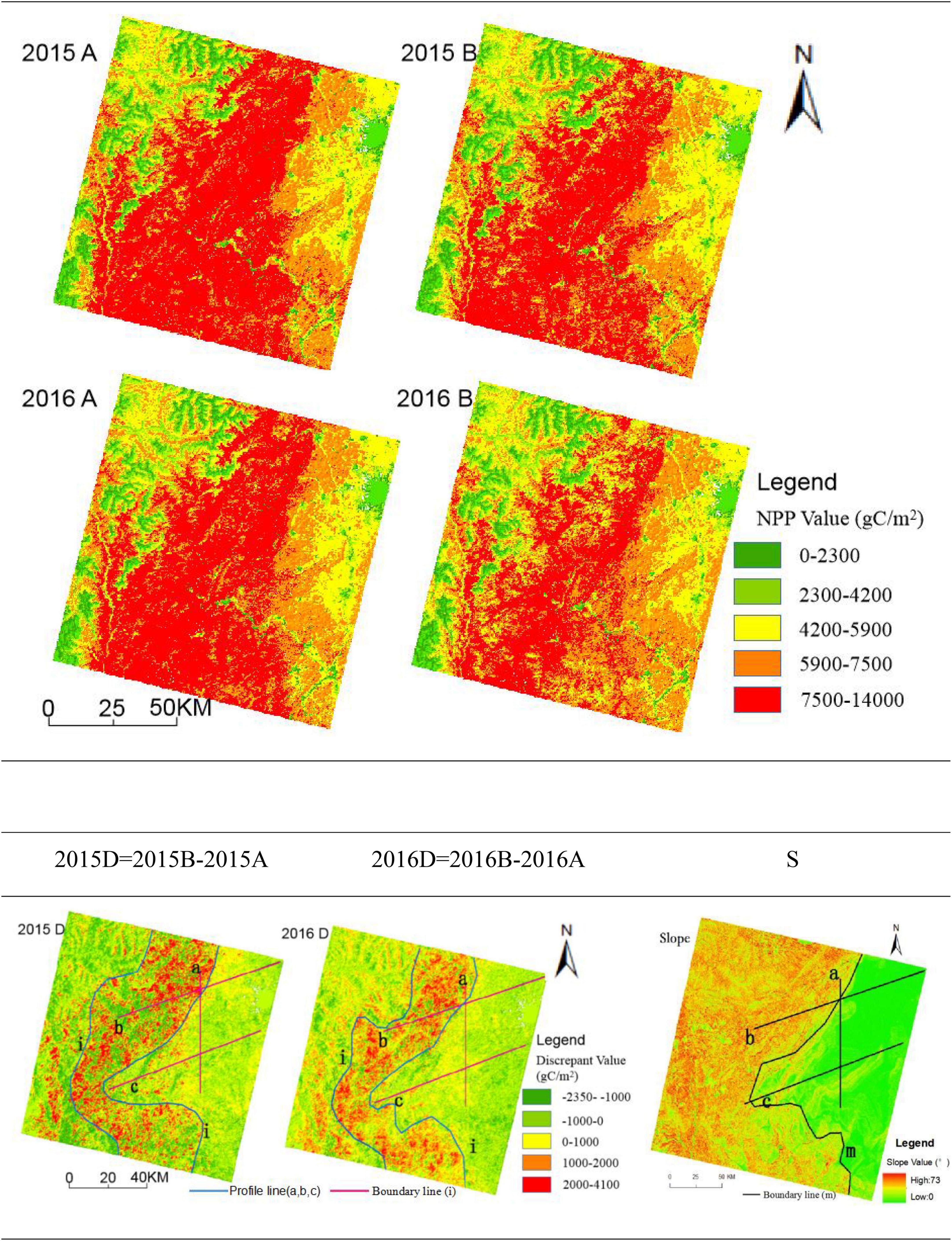
Figure 4. Discrepant data and profile line distribution of the improved CASA model and CASA model estimation results.

The discrepant data between 2015 and 2016 show that while the negative value of the discrepant data is primarily dispersed in the east and northwest of the research region with a modest slope, the positive value is primarily concentrated in the area with a high slope. The reason is that, as seen in Figure 3, the ε_max value of the improved CASA model is greater than that of the CASA model when the sunny slope is less than 35° or the shady slope is less than 26° and smaller than that of the CASA model when the slope is greater than 35 or 26°. As a result, the area with a large slope is where the positive value of the resulting discrepant data is primarily spread, whereas the area with a small slope is where the negative value is disseminated. Second, the high value areas of the discrepant data are concentrated in the areas with a large slope, as can be observed from D (2015), D (2016), and slope data (S), but the eastern parts with relatively smooth terrain are rarely distributed. Despite having a considerable slope, the northwest study area has a low value of different data due to the greater altitude and colder temperatures, which cause less vegetation and lower discrepant data. The borderline (i) west of the discrepant data is the same, showing that other factors, such as climate, have taken the place of the topographic component as the progressive rise in altitude has affected the estimation results. The borderline (i) east of the discrepant data is essentially consistent with the boundary line (m) of the slope, indicating that slope is one of the main factors affecting the estimation results and that the change in the discrepant data is positively correlated with the slope in the easternmost areas of the study area.

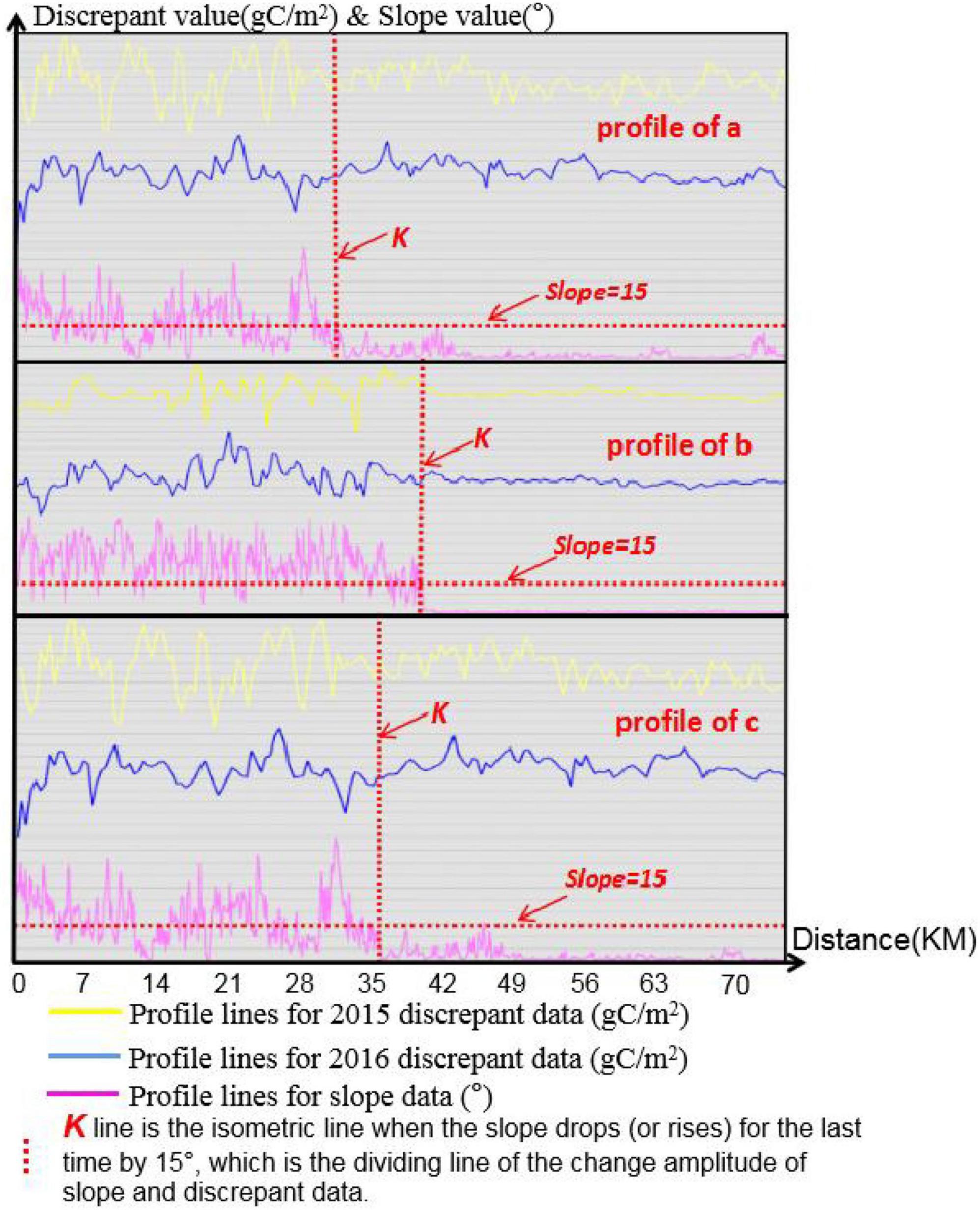
It can be seen from the profiles of the three profile lines (Figures 5a–c) that when the slope rises for the first time or drops to 15° for the last time, the boundary line (K line) of the discrepant data fluctuation will be generated. On the left side of the K line, the discrepant data between 2015 and 2016 and the undulation of the slope are large; on the right side of the K line, the discrepant data and gradient between 2015 and 2016 fluctuate slightly. It shows that the variation value of discrepant data is larger in areas with larger slopes and smaller in areas with smaller slopes. At the same time, the improved CASA model also uses 15° as the dividing point to divide the impact of slope on the ε_max. Therefore, Figures 4, 5 show the distribution characteristics of the estimation results and slopes, which shows the feasibility of the improved CASA model in carbon sequestration estimation.

FIGURE 5

Figure 5. Superposition diagram of the profile line of discrepant data and slope.

Verification of slope aspect

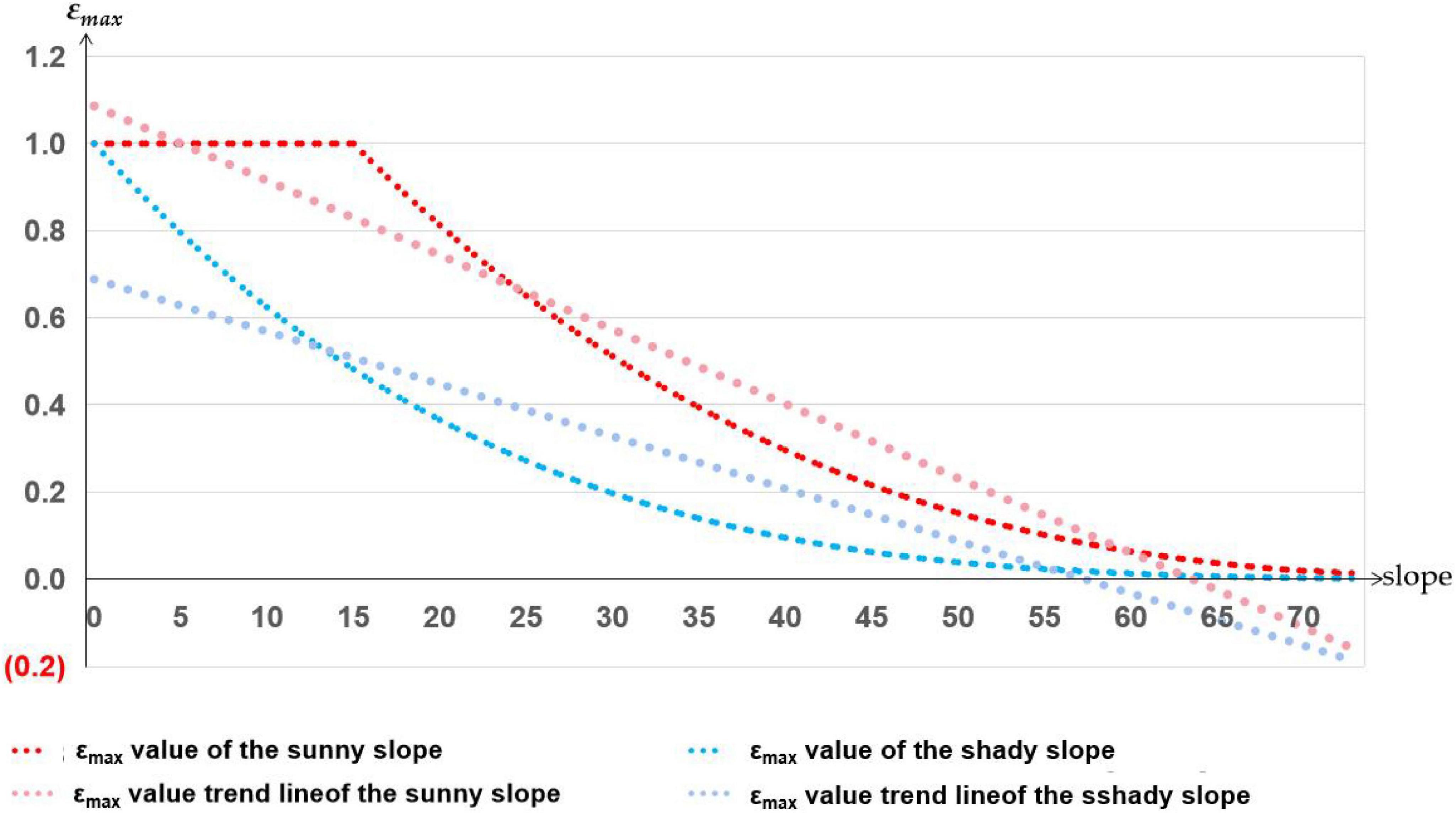
The second difference between the improved CASA model and the CASA model is that the improved model divides the slope aspect into the shady slope and the sunny slope and establishes the functional relationship between the shady slope, sunny slope, and ε_max. To verify the relationship between the discrepant data and the slope aspect, the study counts the area of sunny slopes and shady slopes of the study area, superimposes the discrepant data with the slope aspect map of the study area, and counted the distribution of the discrepant data on the sunny slopes and shady slopes. According to statistical Table 3, the areas of shady slopes (50.26%) and sunny slopes (49.74%) in the study area are the same. If the influence of the slope aspect on ε_max is not considered, the distribution of discrepant data on the shady slope and sunny slope should also be the same. However, the geometric calculation formula of slope aspect and ε_max was established by the improved CASA model, and the sum of ε_max values of the sunny slopes is 1.57 times the sum of ε_max values of the shady slopes (Figure 6). Therefore, without considering the influence of other factors, the ratio of the data value of the discrepant data on the sunny slopes to the data value of the discrepant data on the shady slope is greater than 1.57 because vegetation coverage on the sunny slope is higher than that on the shady slope. According to the data statistics, the distribution discrepant data value of the sunny slope in the study area is 1.94 times that of the shady slope, which proves the influence of the improved slope aspect of the CASA on the estimation result of carbon sequestration.

TABLE 3

Table 3. Statistical table of the distribution of discrepant data on shady slopes and sunny slopes.

FIGURE 6

Figure 6. Relationship between slope and ε_max.

Results

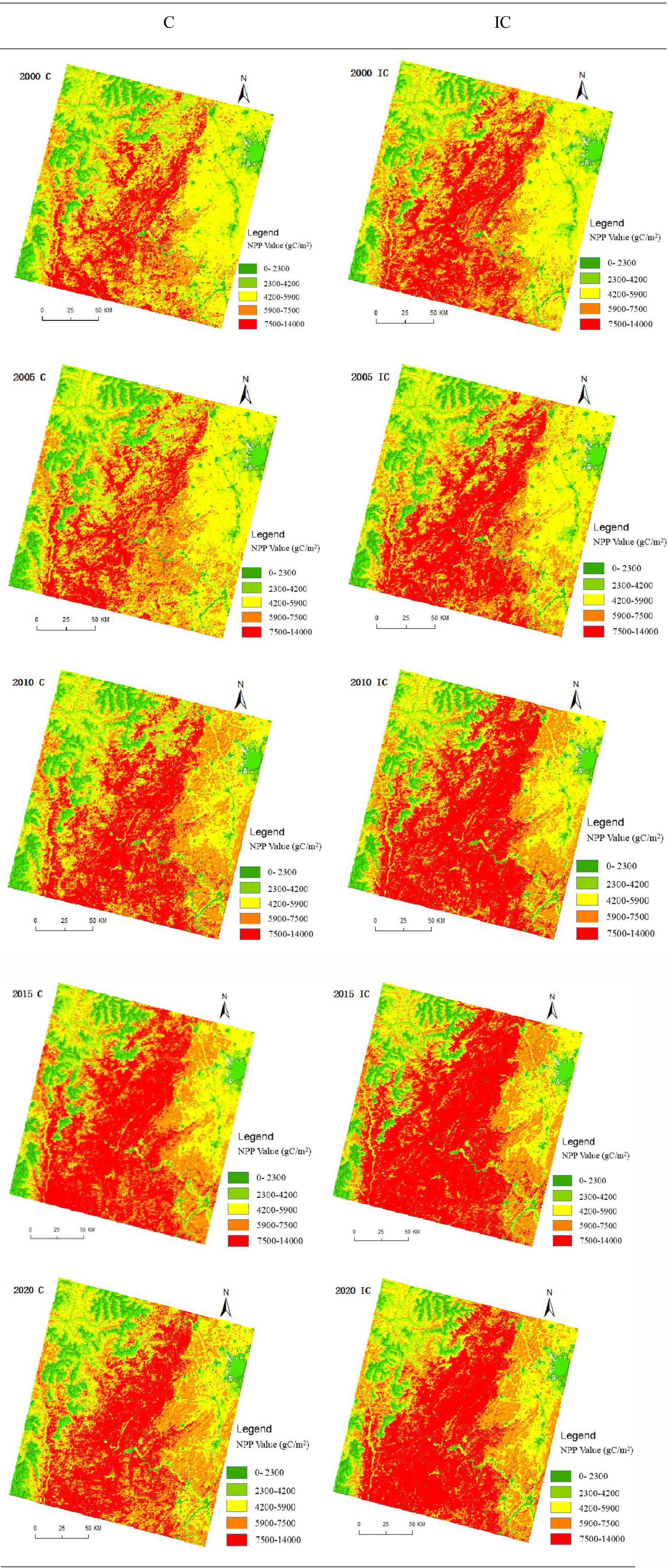
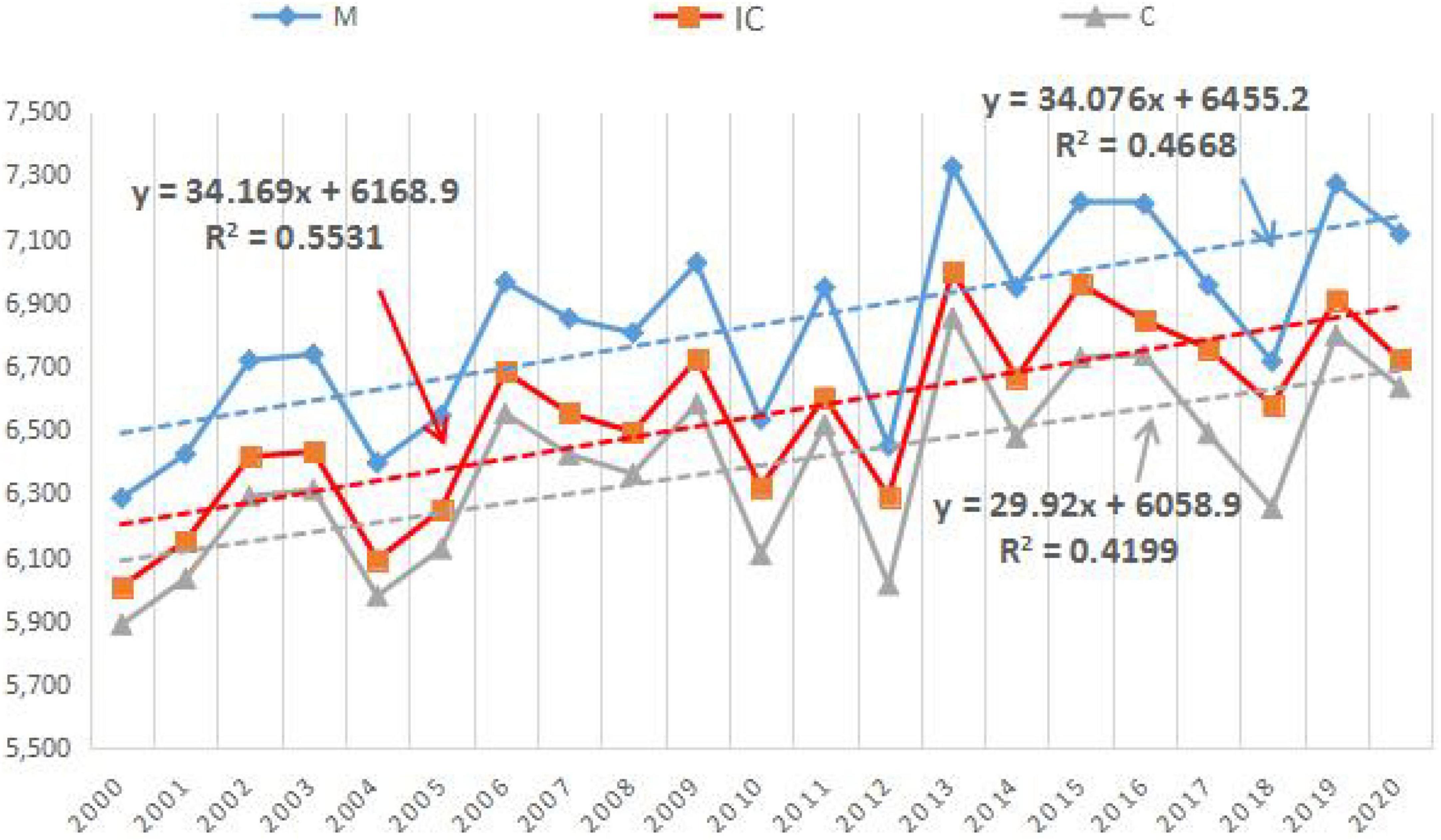
To verify the accuracy of the estimation results of the improved CASA model, the results of vegetation carbon sequestration (IC and C in Figure 7) estimated by the improved CASA model and CASA model in the study area from 2000 to 2020 were compared with the calculation results of NPP products from MODIS data. It should be noted that the estimation result here is not the annual NPP value of the study area, but the author selects remote sensing images with good quality each year according to the quality of remote sensing images in the study area from 2000 to 2020 to estimate the carbon sequestration in the study area. In contrast, MODIS NPP data are synthetic data of 8 days that overlap with the acquisition time of remote sensing images to reduce the estimation error. The accuracy of the improved CASA model was verified by analysing the correlation and the degree of fit among the three. Figure 7 shows only the estimates for 2000, 2005, 2010, 2015, and 2020.

FIGURE 7

Figure 7. Improved CASA model and CASA model estimation results 2000–2020.

According to the basic principle that chloroplasts need to absorb 1.63 g of carbon from the air for every 1 g of organic material produced during photosynthesis (Liu X. et al., 2013; Liu Y. et al., 2013), the total forest carbon sequestration in Sichuan mountain areas from 2000 to 2020 can be estimated by the CASA model, improved CASA model and MODIS data products (Table 4).

TABLE 4

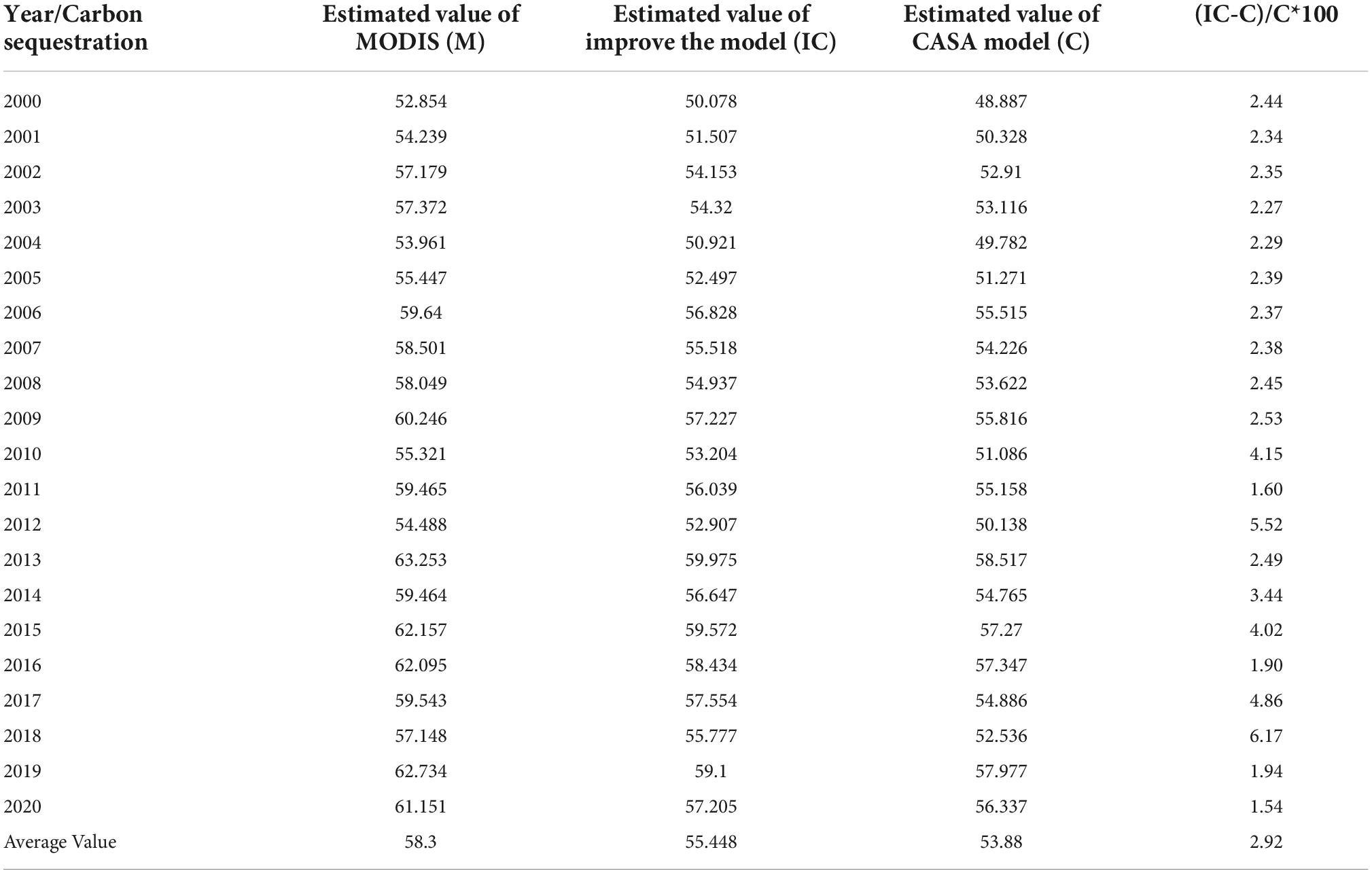
Table 4. Estimation of vegetation carbon sequestration in the study area from 2010 to 2020 (unit: 10,000 tons).

Table 4 shows that the calculated value of MODIS data (M) > estimated value of improved CASA model (IC) > estimated value of CASA model (C), the estimated average value of improved CASA model is 554,48 tons, the estimated average value of CASA model is 538,800 tons, and the mean value of MODIS data is 583,000 tons. The improved model increased the estimated mean value by 2.92%. This assumes that the estimated value of MODIS data is the measured value and compares the improved CASA model and the relationship between the estimated value of the CASA model and MODIS data to determine the accuracy of the estimation of the improved CASA model.

Because the impact of slope and aspect on vegetation carbon sequestration estimation is relatively stable, its impact will not be affected by the external temperature and precipitation. Therefore, if the difference in the estimation results of the three methods is relatively stable and the variation trend is the same, it can show the accuracy of the improved model in the estimation of forest carbon sequestration in mountainous areas. As shown in Figure 8, the trend lines of vegetation carbon sequestration estimated by the three methods are consistent, and the changing trend is consistent. The trend line fitting degree index of the improved CASA model (R² = 0.5531) is the largest and the fitting degree is the best.

FIGURE 8

Figure 8. Trends of forest carbon sequestration estimated by the three methods from 2000 to 2020.

Assuming that the MODIS data are measured values, the correlation between the improved CASA model, the estimated results of the CASA model, and the calculated results of the MODIS data is calculated to determine whether the estimated results of the improved CASA model are accurate. In Figure 9, the correlation between the estimated results of the improved CASA model and MODIS data (R² = 0.9596) is higher than that between the estimated results of the CASA model and the calculated results of MODIS data (R² = 0.9465). Thus, the accuracy of the improved CASA model in estimating forest carbon sequestration in mountainous areas was illustrated.

FIGURE 9

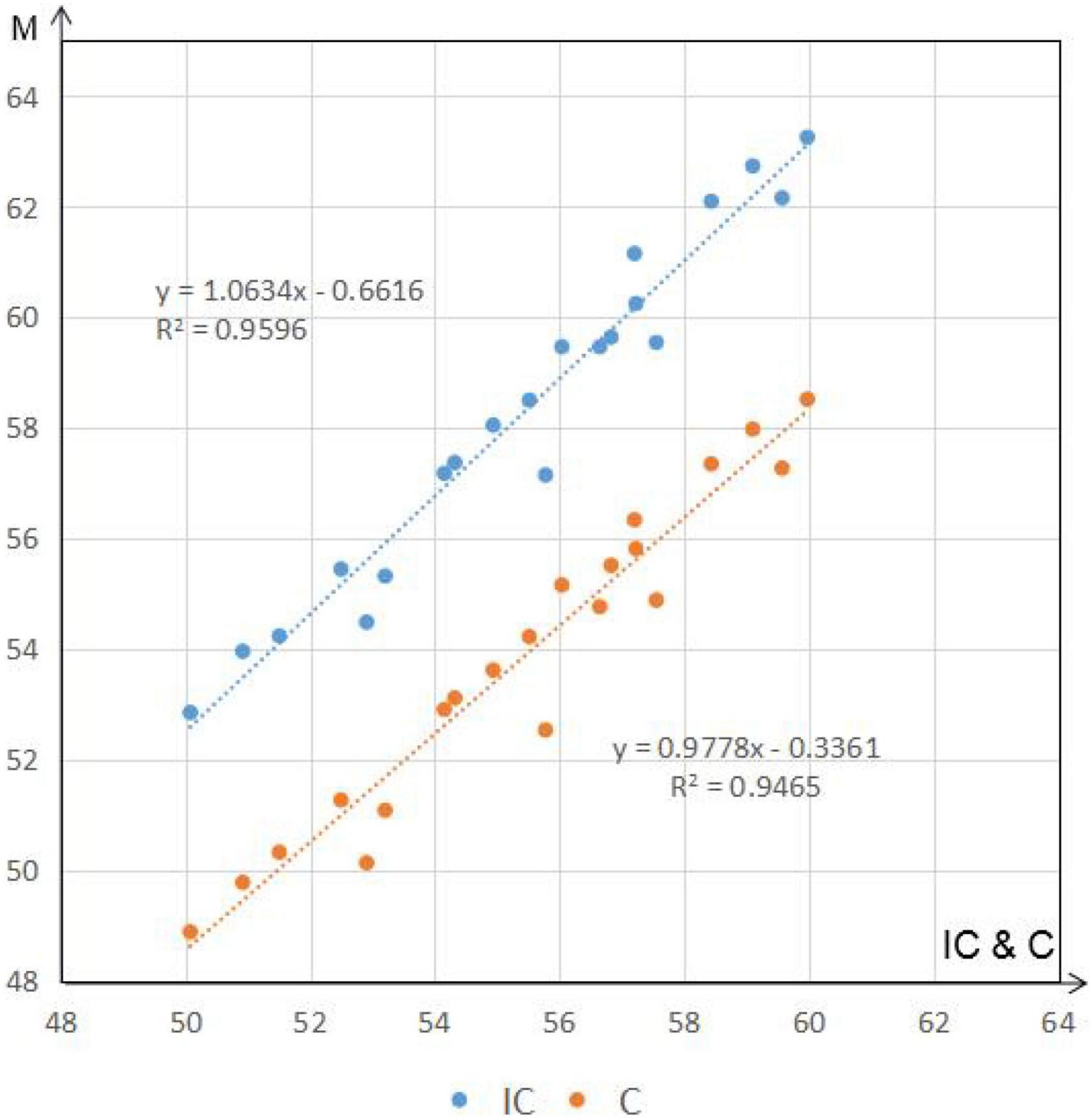
Figure 9. Correlation of the NPP value of the improved model with the estimated value of the CASA model and the NPP value of the MODIS products.

Discussion

Compared with other improved CASA models, the improved CASA model’s biggest characteristic is to build the ε_max and vegetation types, slope, and slope to the function relation, overcome the CASA model for the ε_max unified assigned to estimate the precision of the impact of makesup for the CASA model to estimate does not consider terrain factors. After verifying the feasibility of the improved CASA model through statistical analysis of the data and comparing the estimation results of the improved CASA model, CASA model, and MODIS NPP product, it is found that the calculation results of the improved CASA model are between the CASA model and MODIS data product. Because MODIS data apply to the global-large scale spatial range, the estimated result of carbon sequestration is larger than the actual (Steinberg et al., 2006; Chen et al., 2008; Li et al., 2010; Zhu et al., 2018). However, the estimation results of the CASA model are mainly combined with climate conditions such as temperature and precipitation, and due to the influence of mountainous terrain factors, the estimated results are slightly smaller than the actual carbon sequestration value (As-syakur et al., 2010; Li et al., 2019a,b; Meraj et al., 2022). Therefore, the estimation results of the improved CASA model have the best fitting degree and good correlation between the CASA model and MODIS data products, indicating that the improved CASA model has improved the estimation accuracy of the model to a certain extent.

However, the improved CASA model also has shortcomings: the improved CASA model requires high-quality remote sensing image data, especially a low proportion of cloud pixels in the image (Kuang et al., 2020; Yong et al., 2022). Because cloud pixels have a great impact on the acquisition of the vegetation index, the number of cloud pixels directly affects the accuracy of estimation, and remote sensing images more or less have cloud pixels. Therefore, to improve the accuracy of carbon sequestration estimation, it is necessary to select remote sensing images with fewer cloud pixels and good quality to estimate vegetation sequestration, which increases the workload to a certain extent; Second, in mountainous areas with a large degree of relief, there are large differences in temperature, humidity, and precipitation between the top and bottom of the slope (Wang et al., 2018). Therefore, when the improved CASA model is used to analyse meteorological data, it is easy to cause inconsistencies and uncertainties in the accuracy of interpolation results. The greater the degree of relief is, the greater the uncertainty. The improved CASA model has improved the accuracy of carbon sequestration estimation of vegetation in mountainous areas with a large degree of relief but has not significantly improved the accuracy of carbon sequestration estimation of vegetation in plains and hills with a relatively high degree of relief. The solution to this problem also depends on appropriately increasing the number of meteorological stations and the reasonable spatial layout of meteorological stations. Moreover, the change in land use types will lead to the change in vegetation types in space (Li, 2021; Wang et al., 2022), thus leading to the change in the maximum light energy utilization rate of vegetation. On a short time scale, due to the small change in vegetation types, the estimated result image of the improved CASA model is small. If it is on a longer time scale, it will have a greater impact on the estimation results. The impact of slope on the carbon sequestration of vegetation is the impact of soil properties on the carbon sequestration of vegetation. Soil properties include soil organic matter content, soil thickness, soil moisture, and other factors. In general, the greater the slope is, the smaller the soil thickness and the lower the soil organic matter and soil water content. Due to the flourishing vegetation in mountain areas, it is difficult to obtain soil property information by using remote sensing technology. However, the spatial resolution of soil information today is low, and the precision is not high, which cannot meet the research needs. Therefore, the paper uses slope to reflect the impact of soil properties on the carbon sequestration of vegetation from the side, which will also affect the estimation accuracy to a certain extent. The next step will be to strengthen the research of remote sensing technology in information acquisition of high vegetation areas to overcome the shortcomings of the improved CASA model.

Conclusion

The improved CASA model overcomes the shortcomings of the CASA model in that the ε_max is uniformly assigned and the influence of terrain factors is not considered. The calculation method of key parameters is improved, and the functional relation between vegetation, aspect, slope, and ε_max of vegetation is established. After verifying the feasibility of the improved model, and comparing the estimation results of the three methods, it is found that the improved CASA model has the best fitting degree and high correlation. The improved CASA model is helpful to more accurately grasp the ecological carbon sequestration capacity of mountain vegetation.

Data availability statement

The raw data supporting the conclusions of this article will be made available by the authors, without undue reservation.

Author contributions

XH, LH, and ZH: conceptualization and methodology. XH and LH: writing—original draft preparation and writing—review and editing. XN and PL: visualization. HY and PL: data curation. All authors have read and agreed to the published version of the manuscript.

Funding

This research was supported by Natural Science Foundation of Sichuan Province (2022NSFSC1040) and supported by the Independent Research Project of the State Key Laboratory of Geohazard Prevention and Geoenvironment Protection Independent Research Project (SKLGP2021Z003).

Acknowledgments

Thank you for the free data provided by the platform and the scholars who provided references, as well as the State Key Laboratory of Geohazard Prevention and Geoenvironment Protection and Chengdu University of Technology for their support.

Conflict of interest

The authors declare that the research was conducted in the absence of any commercial or financial relationships that could be construed as a potential conflict of interest.

Publisher’s note

All claims expressed in this article are solely those of the authors and do not necessarily represent those of their affiliated organizations, or those of the publisher, the editors and the reviewers. Any product that may be evaluated in this article, or claim that may be made by its manufacturer, is not guaranteed or endorsed by the publisher.

Footnotes

1. ^ http://www.gscloud.cn/
2. ^ http://data.cma.cn/
3. ^ https://www.resdc.cn/Default.aspx

References

Anikó, K., Hrvoje, M., Laura, D., Mislav, A., Tomáš, H., and Zoltán, B. (2017). Identification of years with extreme vegetation state in central Europe based on remote sensing and meteorological data. South East Eur. For. 8, 1–20.

Google Scholar

As-syakur, A. R., Osawa, T., and Adnyana, I. W. S. (2010). Medium spatial resolution satellite imagery to estimate gross primary production in an Urban Area. Remote Sens. 2:1496.

Google Scholar

Cai, W., Wenping, Y., Shunlin, L., Liu, S., Dong, W., Chen, Y., et al. (2014). Large differences in terrestrial vegetation production derived from satellite-based light use efficiency models. Remote Sens. 6, 8945–8965. doi: 10.3390/rs6098945

CrossRef Full Text | Google Scholar

Cai, Y., Zheng, J., Du, M., Mu, C., and Peng, J. (2018). “Grassland npp monitoring based on multi-source remote sensing data fusion,” in Proceedings of the ISPRS technical commission III midterm symposium on developments, technologies and applications in remote sensing, 371–376.

Google Scholar

Chen, F., Li, H., and Liu, Y. (2018). Temporal and spatial differentiation of vegetation NPP in mountainous areas of Southern Yunnan and its influencing factors based on GIS and CASA: Taking Yuanyang County, Yunnan province as an example. J. Ecol. 37, 2148–2158. doi: 10.13292/j.1000-4890.201807.003

CrossRef Full Text | Google Scholar

Chen, J., Yan, H., Wang, S., Gao, Y., Huang, M., Wang, J., et al. (2014). Estimation of total primary productivity of China’s terrestrial ecosystem by VPM remote sensing model. Quat. Res. 34, 732–742.

Google Scholar

Chen, L., Gao, Y., Li, L., Liu, Q., and Gu, X. (2008). Forest NPP estimation based on MODIS data under cloudless condition. Sci. China Ser. D Earth Sci. 51, 331–338.

Google Scholar

Chen, S., Guo, B., Zhang, R., Zang, W., Wei, C., Wu, H., et al. (2021). Quantitatively determine the dominant driving factors of the spatial–temporal changes of vegetation NPP in the Hengduan Mountain area during 2000-2015. J. Mt. Sci. 18, 427–445.

Google Scholar

Chen, T., Peng, L., Liu, S., and Wang, Q. (2017). Spatio-temporal pattern of net primary productivity in Hengduan Mountains area, China: Impacts of climate change and human activities. Chin. Geogr. Sci. 27, 948–962.

Google Scholar

Chen, X., and Zeng, Y. (2016). Temporal and spatial variation of vegetation NPP and its relationship with climatic factors in subtropical mountainous and hilly region: A case study of Hunan province. Acta Geogr. Sin. 1, 35–48.

Google Scholar

Christian, K., and Jens, P. (2011). A definition of mountains and their bioclimatic belts for global comparisons of biodiversity data. Alp. Bot. 121:73. doi: 10.1007/s00035-011-0094-4

CrossRef Full Text | Google Scholar

Du, M., Zheng, J., Ren, X., Cai, Y., Mu, C., and Yan, K. (2018). Effects of topography on the distribution pattern of grassland net primary productivity in Changji prefecture, Xinjiang. Acta Zool. Sin. 38, 4789–4799.

Google Scholar

Du, B., Alattentua, Bao, G., Wang, N., and Lin, K. (2021). Simulation of net primary productivity of Xilin Gol grassland based on CASA model. Res. Soil Water Conserv. 28, 293–300. doi: 10.13869/j.cnki.rswc.2021.05.034

CrossRef Full Text | Google Scholar

Du, S., Liu, L., Liu, X., and Hu, J. (2017). Response of canopy solar-induced chlorophyll fluorescence to the absorbed photosynthetically active radiation absorbed by chlorophyll. Remote Sens. 9:911. doi: 10.3390/rs9090911

CrossRef Full Text | Google Scholar

Fan, Y. (2018). Temporal and spatial variation of vegetation carbon source/sink and its response to climate change in Hexi Corridor. Lanzhou: Northwest Normal University.

Google Scholar

Field, C. B., Behrenfeld, M. J., Randerson, J. T., and Falkowski, P. (1998). Primary production of the biosphere: Integrating terrestrial and oceanic components. Science 281, 237–240. doi: 10.1126/science.281.5374.237

PubMed Abstract | CrossRef Full Text | Google Scholar

Han, H. (2020). Relationship between vegetation phenology and net primary productivity (NPP) and its response to climate change in the Loess Plateau. Shanxi: Shaanxi Normal University.

Google Scholar

He, L., Li, A., Yin, G., and Bian, J. (2019). Retrieval of grassland aboveground biomass through inversion of the prosail model with modis imagery. Remote Sens. 11:1597. doi: 10.3390/rs11131597

CrossRef Full Text | Google Scholar

He, N., Zhang, J., Liu, C., Xu, L., Chen, Z., Liu, Y., et al. (2018). Research progress on spatial pattern and influencing factors of forest ecosystem traits–integrated analysis based on transect in eastern China. J. Ecol. 38, 6359–6382.

Google Scholar

Hicke, J. A., Asner, G. P., Randerson, J. T., and Tucker, C. J. (2002). Trends in North American net primary productivity derived from satellite obser-vations, 1982–1998. Glob. Biogeochem. Cycles 16, 1019–1040.

Google Scholar

Jiang, H., Yu, J., Jiang, S., Huang, B., and Li, Y. (2021). Remote sensing estimation and analysis of NPP of vegetation in Fujian province based on CASA model and SEVI index. J. Hainan Univ. 39, 372–382.

Google Scholar

Jiang, H., Yuan, Y., and Wang, S. (2019). The performance evaluation and application of shadow elimination vegetation index (SEVI) in removing topographic umbra and falling shadow interference. J. Geoinform. Sci. 21, 1975–1984.

Google Scholar

Körner, C., Urbach, D., and Paulsen, J. (2021). Mountain definitions and their consequences. Alp. Bot. 131, 1–5. doi: 10.1007/S00035-021-00265-8

CrossRef Full Text | Google Scholar

Kuang, Q., Yuan, Q., Han, J., Leng, R., Wang, Y., Zhu, K., et al. (2020). A remote sensing monitoring method for alpine grasslands desertification in the eastern Qinghai–Tibetan Plateau. J. Mt. Sci. 17, 1423–1437.

Google Scholar

Lan, F., Wenmin, Q., Lunche, W., Aiwen, L., and Ming, Z. (2018). Comparison of artificial intelligence and physical models for forecasting photosynthetically-active radiation. Remote Sens. 10, 1855–1855. doi: 10.3390/rs10111855

CrossRef Full Text | Google Scholar

Li, A., Bian, J., Lei, G., and Huang, C. (2012). Estimating the maximal light use efficiency for different vegetation through the CASA model combined with time-series remote sensing data and ground measurements. Remote Sens. 4, 3857–3876. doi: 10.3390/rs4123857

CrossRef Full Text | Google Scholar

Li, C. (2021). Accuracy improvement method and influencing factors of aboveground biomass estimation of mid-subtropical forests by remote sensing. Ph.D. thesis. Jiangsu: Nanjing Forestry University. doi: 10.27242/-d.cnki.gnjlu.2021.000024

CrossRef Full Text | Google Scholar

Li, C., Cao, H., Fan, Y., Han, H., Sun, H., and Wang, Y. (2019a). Remote sensing estimation and analysis of NPP based on corrected CASA model: A case study of Hexi corridor. Acta Ecol. Sin. 39, 1616–1626.

Google Scholar

Li, C., Han, H., Fan, Y., Cao, H., Wang, Y., and Sun, H. (2019b). Variation and scenario simulation of NPP in wudaoliang region of qinghai-tibet plateau based on Biome-BGCmodel. Geogr. Sci. 39, 1330–1339. doi: 10.13249/-j.cnki.sgs.-2019.08.015

CrossRef Full Text | Google Scholar

Li, C., Yang, S., Wu, F., Xu, Y., and Cui, X. (2022). Temporal and spatial differentiation of carbon emissions from energy consumption and carbon sequestration by vegetation in China under the “double carbon” background. China Environ. Sci. 42, 1945–1953.

Google Scholar

Li, G., Zhang, H., Fan, W., Zhang, H., and Xin, X. (2010). Accuracy verification and analysis of MODIS/fAPAR in hulunbuir grassland area. J. Agric. Eng. 26, 217–224+8.

Google Scholar

Li, H., Qu, Y., Zeng, X., Zhang, H., Cui, L., and Luo, C. (2021). Dynamic response of the vegetation carbon storage in the sanjiang plain to changes in land use/cover and climate. Herit. Sci. 9:134. doi: 10.1186/S40494-021-00605-1

CrossRef Full Text | Google Scholar

Li, M., Shang, G., Zhou, P., and Deng, L. (2021). Spatial distribution and influencing factors of ecosystem carbon storage in the Loess Plateau. Acta Ecol. Sin. 41, 6786–6799.

Google Scholar

Li, X. (2013). Remote sensing estimation of NPP in Heihe river basin and analysis of its spatiotemporal change characteristics. Shaanxi: Shaanxi Normal University.

Google Scholar

Li, Y., Tao, S., Li, R., et al. (2021). Spatial and temporal evolution of net primary productivity in Liaoning province and its response to topographic factors. J. Meteorol. Environ. 37, 107–112.

Google Scholar

Liu, M., Jiao, J., Pan, J., Song, J., Che, Y., and Li, L. (2020). Changes in the spatiotemporal pattern of net primary productivity (npp) and its driving factors in qinghai province. Acta Ecol. 40, 5306–5317.

Google Scholar

Liu, X., Ren, Z., and Lin, Z. (2013). Dynamic evaluation of carbon sequestration and oxygen release value of ecosystem in qinghai tibet plateau. Geogr. Res. 32, 663–670.

Google Scholar

Liu, Y., Huang, B., Yi, C., Chen, T., Yu, J., and Qu, L. (2013). Remote sensing simulation and analysis of vegetation net primary productivity based on terrain correction. J. Agric. Eng. 29, 130–141.

Google Scholar

Meraj, G., Kanga, S., Ambadkar, A., Kumar, P., Singh, S. K., Farooq, M., et al. (2022). Assessing the yield of wheat using satellite remote sensing-based machine learning algorithms and simulation modeling. Remote Sens. 14, 3005–3005.

Google Scholar

National Meteorological Information Center [NMC] (2018). China meteorological data service centre. Beijing: National Meteorological Information Center [NMC].

Google Scholar

Pan, J., and Xu, B. (2020). Simulation of NPP spatial distribution of potential vegetation in China. Chin. J. Ecol. 39, 1001–1012. doi: 10.13292/j.1000-4890.202003.030

CrossRef Full Text | Google Scholar

Peng, C., Zhou, Q., Meng, H., Li, M., Zhou, L., and Liu, X. (2021). Sensitivity analysis of landscape ecology and identification of key restoration areas in Chongqing section of three gorges reservoir based on LECI. Soil Water Conserv. Res. 28, 325–330+339+4.

Google Scholar

Peng, S., Guo, Z., and Wang, B. (2000). Estimation of light utilization rate of vegetation in Guangdong by GIS and RS. Acta Zool. Sin. 6, 903–909.

Google Scholar

Price, M. F., Arnesen, T., Erik, G., and Metzger, M. J. (2019). Mapping mountain areas: Learning from global, European and Norwegian perspectives. J. Mt. Sci. 16, 1–15.

Google Scholar

Shen, X., Wang, P., Wang, W., Wang, S., Xie, R., Wang, Y., et al. (2022). Summary of research methods on net carbon sink capacity of coastal salt marsh. J. Ecol. 41, 792–803. doi: 10.13292/j.1000-4890.202203.009

CrossRef Full Text | Google Scholar

Singh, R., Semwal, D. P., Rai, A., and Chhikara, R. S. (2002). Small area estimation of crop yield using remote sensing satellite data. Int. J. Remote Sens. 23, 49–56. doi: 10.1080/01431160010014756

CrossRef Full Text | Google Scholar

Steinberg, D. C., Goetz, S. J., and Hyer, E. J. (2006). Validation of MODIS F/Sub PAR/products in boreal forests of Alaska. IEEE Trans. Geosci. Remote Sens. 44, 1818–1828.

Google Scholar

Sun, Q., Feng, X., and Xiao, X. (2014). Spatial and temporal pattern of net primary productivity of vegetation in Wuling mountain area and its relationship with topographic factors. J. Geo Inf. Sci. 16, 915–924.

Google Scholar

Sun, Q., Li, B., Li, F., Zhang, Z., Ding, L., Zhang, T., et al. (2016). Advances in estimation of net primary productivity of vegetation in the three-river headwaters region. Acta Geogr. Sin. 71, 1596–1612.

Google Scholar

Sun, Z., and Xie, S. (2021). Spatial-temporal variation and factor detection of net primary productivity in yunnan province based on geographic detector. Chin. J. Ecol. 40, 3836–3848. doi: 10.13292/J.1000-4890.202111.033

CrossRef Full Text | Google Scholar

Tang, W., Qin, J., Yang, K., Niu, X., Min, M., and Liang, S. (2017). An efficient algorithm for calculating photosynthetically active radiation with MODIS products. Remote Sens. Environ. 194, 146–154.

Google Scholar

Wang, B., Wang, J., Yang, Y., Chang, S., Chang, X., and Liu, A. (2013). Improved algorithm of photosynthetic active radiation absorption component and maximum light utilization of vegetation. Acta Pratacult. Sin. 22, 220–228.

Google Scholar

Wang, B., Zhou, S., Jing, Y., Song, J., and Wang, R. (2021). Temporal and spatial changes of vegetation phenology in shanxi province and the impact of topography on phenology. J. Ecol. 40, 1839–1848. doi: 10.13292/-j.1000-4890.202106.030

CrossRef Full Text | Google Scholar

Wang, H., Luo, G., Wang, W., Pachikin, K., Li, K., Zheng, H., et al. (2019). Inversion of farmland soil moisture in the middle and lower reaches of the Syr Darya based on multi-source remote sensing data. J. Nat. Resour. 34, 2717–2731.

Google Scholar

Wang, J., Feng, L., Palmer, P. I., Liu, Y., Fang, S., Bösch, H., et al. (2020). Large Chinese land carbon sink estimated from atmospheric carbon dioxide data. Nature 586, 720–723.

Google Scholar

Wang, J., Zhao, A., and Hu, X. (2021). Spatial and temporal distribution of net primary productivity of vegetation in Beijing. Tianjin and Hebei and analysis of natural driving factors. J. Ecol. Environ. 30, 1158–1167. doi: 10.16258/j.cnki.1674-5906.2021.06.006

CrossRef Full Text | Google Scholar

Wang, L., Gong, W., Feng, L., Lin, A., Hu, B., and Zhou, M. (2015). Estimation of hourly and daily photosynthetically active radiation in Inner Mongolia, China, from 1990 to 2012. Int. J. Climatol. 35, 3120–3131. doi: 10.1002-/joc.4197

CrossRef Full Text | Google Scholar

Wang, L., Gong, W., Zhang, M., and Ma, Y. (2013). Study on dynamic monitoring of vegetation NPP in Wuhan area. J. Wuhan Univ. 38, 548–552. doi: 10.13203/j.whigis2013.-05.004

CrossRef Full Text | Google Scholar

Wang, W., Zou, W., and Wang, R. (2022). Land space planning path and governance mechanism of urban agglomeration under the goal of “double carbon”. Environ. Protect. 50, 64–69. doi: 10.14026/-j.cnki0253-9705.2022Z1.011

CrossRef Full Text | Google Scholar

Wang, Y., Cao, G., Wang, Y., Xu, L., Zhang, W., and Wang, X. (2018). Canopy transpiration and its influencing factors of larch huabei artificial forest in the southern side of liupan mountain. Chin. J. Appl. Ecol. 29, 1503–1514. doi: 10.13287/j.1001-9332.201805.006

PubMed Abstract | CrossRef Full Text | Google Scholar

Wang, Y., Xu, X., Huang, L., Yang, G., Fan, L., Wei, P., et al. (2019). An improved CASA model for estimating winter wheat yield from remote sensing images. Remote Sens. 11:1088. doi: 10.3390/rs11091088

CrossRef Full Text | Google Scholar

Xia, A., Wang, Y., and Hao, Y. (2020). Advances in estimating carbon storage of grassland vegetation in complex terrain using remote sensing. Acta Ecol. Sin. 40, 6338–6350.

Google Scholar

Xing, X., Xu, X., Zhang, X., Zhou, C., Song, M., Shao, B., et al. (2010). Simulating net primary production of grasslands in northeastern Asia using MODIS data from 2000 to 2005. J. Geogr. Sci. 20, 193–204.

Google Scholar

Xu, J., Chen, D., Li, W., and Wei, W. (2019). Research on net primary productivity of vegetation in gannan prefecture based on light energy utilization rate model. Grass Sci. 36, 2455–2465.

Google Scholar

Xu, Y., Xiao, F., and Yu, Y. (2020). A review on the temporal and spatial distribution of net primary productivity of forest ecosystems in China and its response to climate change. J. Ecol. 40, 4710–4723.

Google Scholar

Yan, D., Li, J., Xue, Y., Qi, L., and Luan, Z. (2022). Inversion of vegetation biophysical characteristics in jiangsu province based on sentinel-2. J. Environ. Sci. 42, 70–79. doi: 10.13671/j.hjkxxb.2021.0488

CrossRef Full Text | Google Scholar

Yan, P., Jin, H., Li, W., Chi, H., and Zhao, Y. (2018). An improved phenology-based CASA model for estimating net primary production of forest in central China based on Landsat images. Int. J. Remote Sens. 39, 7664–7692.

Google Scholar

Yang, L. (2019). Evaluating the responses of net primary productivity and carbon use efficiency of global grassland to climate variability along an aridity gradient. Sci. Total Environ. 652, 671–682. doi: 10.1016/j.scitotenv.2018.10.295

PubMed Abstract | CrossRef Full Text | Google Scholar

Yang, Y., Li, L., Wang, B., Liu, A., and Wang, M. (2015). Simulation of net primary productivity of vegetation in Xilin Gol grassland based on improved CASA model. J. Ecol. 34, 2344–2352. doi: 10.13292/j.1000-4890.2015.0203

CrossRef Full Text | Google Scholar

Yong, L., Xiu, H., Fu, W., Xu, Y., Zhang, Y., Tang, S., et al. (2022). Estimation of terrestrial net primary productivity in China from fengyun-3D satellite data. J. Meteorol. Res. 36, 401–416.

Google Scholar

Yu, H., Ni, W., Zhang, Z., Sun, G., and Zhang, Z. (2020). Regional forest mapping over mountainous areas in northeast china using newly identified critical temporal features of sentinel-1backscattering. Remote Sens. 12:1485. doi: 10.3390/rs12091485

CrossRef Full Text | Google Scholar

Zhang, J., and Ren, Z. (2016). Spatial and temporal pattern and causes of net primary productivity of vegetation in the Han river basin. J. Ecol. 36, 7667–7677.

Google Scholar

Zhang, M., Jiang, W., Chen, Q., and Liu, X. (2012). Simulation of the maximum solar energy utilization of various types of grassland comprehensive sequential classification system based on the improved CASA model. Grassl. Lawn 32, 60–66. doi: 10.13817/j.cnki.cyycp.2012.04.017

CrossRef Full Text | Google Scholar

Zhang, Q., Zhang, L., He, H., Han, S., Li, Y., Ou, Y., et al. (2014). Inversion study on maximum solar energy utilization of vegetation based on vorticity related flux data. Quat. Res. 34, 743–751.

Google Scholar

Zhang, R., Guo, J., and Zhang, Y. (2020). Spatial distribution pattern of net primary productivity (NPP) of grassland in Xinjiang and its response to climate change. J. Ecol. 40, 5318–5326.

Google Scholar

Zhang, S., Deng, W., Hu, M., Zhang, H., Wang, Z., and Peng, L. (2022). Identification and differentiation analysis of human nature interaction in transitional geographical space in mountainous areas. J. Geogr. 77, 1225–1243. doi: 10.11821/dlxb202205013

CrossRef Full Text | Google Scholar

Zhang, W., Li, A., and Jiang, X. (2013). Quantitative bounds of China’s mountain spatial range based on DEM. Geogr. Geogr. Inf. Sci. 29, 58–63. doi: 10.13227/j.hjkx.202109031

PubMed Abstract | CrossRef Full Text | Google Scholar

Zhang, Y., and Zhang, X. (2017). Estimation of net primary productivity of different forest types based on improved CASA model in Jing-Jin-Ji region, China. J. Sustain. For. 36, 568–582. doi: 10.1080/105498-11.2017.1314971

CrossRef Full Text | Google Scholar

Zhang, Y., Yuan, Q., Fang, L., Han, Y., Zhu, Q., Qi, L., et al. (2021). Spatial and temporal pattern of net primary productivity of high-altitude spruce fir forests in changbai mountain nature reserve and its driving factors. J. Ecol. 40, 3483–3492. doi: 10.13292/j.1000-4890.20211.013

CrossRef Full Text | Google Scholar

Zhang, Z., and Min, M. (2022). Study on the spatial-temporal differentiation of vegetation productivity and its relationship with topographic factors in Yili Area. J. Cent. China Norm. Univ. 54, 711–720. doi: 10.19603/j.cnki.1000-1190.2020.04.022

CrossRef Full Text | Google Scholar

Zhao, R., Huang, X., Yun, W., Wu, K., Chen, Y., Wang, S., et al. (2022). Key issues in the field of natural resource management under the goal of carbon peaking and carbon neutralization. J. Nat. Resour. 37, 1123–1136.

Google Scholar

Zhu, W., Pan, Y., He, H., Deyong, Y., and Haibo, H. (2006). Simulation of maximum light use efficiency for some typical vegetation types in China. Chin. Sci. Bull. 51, 457–463. doi: 10.1007/s11434-006-0457-1

CrossRef Full Text | Google Scholar

Zhu, L., and Yuan, J. (2019). Spatial and temporal distribution of net primary productivity of vegetation in beijing tianjin hebei region and its relationship with topographic factors. Sci. Technol. Bull. 35, 197–203. doi: 10.13774/j.cnki.kjtb.2019

CrossRef Full Text | Google Scholar

Zhu, Y., Du, L., Xie, Y., Liu, K., Gong, F., Dan, Y., et al. (2018). Accuracy evaluation of different meteorological interpolation methods and their impact on grassland NPP estimation. Soil Water Conserv. Res. 25, 160–167. doi: 10.13869/j.cnki.rswc.2018.06.024

CrossRef Full Text | Google Scholar

Zhu, Y., Du, L., Xie, Y., Liu, K., Gong, F., Dan, Y., et al. (2019). Temporal and spatial characteristics of grassland net primary productivity and its climate response in Ningxia from 2000 to 2015. Acta Ecol. 39, 518–529.

Google Scholar