Assessment of Aesthetic Quality of Urban Landscapes by Integrating Objective and Subjective Factors: A Case Study for Riparian Landscapes

To improve human well-being, there is increasing awareness of elevating aesthetic benefits by landscape design, planning, and management. However, which landscape features and attributes may be associated with aesthetic value of an urban landscape, human aesthetic preference, and landscape practices is still not clear yet. We proposed a comprehensive aesthetic assessment approach to realise the determination of landscape aesthetic indicators, integration of objective indicators and subjective preferences, and validation of estimations. The approach was based on a four-level landscape aesthetic indicator system from the bottom features up to attributes (landscape naturalness, landscape complexity, plant species diversity, water surface, water clarity, and bank naturalness), component qualities, and finally overall quality. Fourteen metrics that could provide objective visual and spatial characters and ecological implications were identified and quantified to indicate landscape aesthetic features. Landscape aesthetic attributes, vegetation and waterbody component qualities, and overall quality were estimated by integrating objective indicators and human subjective preferences. The approach was applied to a case study of four subareas along an artificially restored riparian buffer in Beijing, China. The results showed that the modelled overall aesthetic quality was determined by both vegetation (accounting for 53%) and waterbody. The higher vegetation quality depended on the higher plant abundance, more vegetation patches, and more vegetation patch types; the higher waterbody quality depended on the clearer water and larger water surface. Compared with other features, vertical vegetation configuration, diversity of patch type and patch shape, and shrub species diversity had greater contribution to the attributes of naturalness, complexity, and plant species diversity, respectively. The modelled vegetation aesthetic attributes were directly validated using the surveyed perceptions, and the modelled vegetation and waterbody aesthetic qualities were indirectly validated by correlating with the main recreational activities. The approach is confirmed to be able to address the questions on determination, integration, and validation of landscape aesthetic indicators in some way. Thus, the approach is expected to be used for other landscapes to offer a framework for landscape practices to improve aesthetic value and cultural service.

Introduction

Landscape, defined as the realm in which humans engage with environmental phenomena and perceive as their surroundings, is a significant component of urban residential satisfaction (Hur et al., 2010; Sahraoui et al., 2016). It is the interaction between landscapes and human viewers within the perceptible realm that gives rise to landscape aesthetic experience (Daniel, 2001). Landscape aesthetic quality, defined as ‘the relative aesthetic excellence of a landscape’ (Daniel, 2001), has been a concern as home or resort sites are selected (de la Fuente de Val et al., 2006; Sahraoui et al., 2016). Aesthetic quality has a profound effect on aesthetic values, which is widely recognised as a cultural service associated with human well-being (Millennium Ecosystem Assessment, 2005; Riechers et al., 2016).

Studies on landscape aesthetics have been conducted since the late 1960s. In the 20th century, there are two main paradigms of landscape aesthetics theory (Gobster et al., 2019). The subjective paradigm (e.g., perception-based, and public preference approaches) perceives landscape quality in the eye of observers and has dominated in landscape preference (general aesthetic favour, not limited at certain time or space) and perception (aesthetic cognition for specific landscapes at certain time) research. The objective paradigm (e.g., expert-based and landscape metrics-based approaches) assesses visual quality inherent to landscape properties and has gained considerable attention in landscape design, planning, and management (Lothian, 1999; Daniel, 2001; Howley, 2011; Jorgensen, 2011; Frank et al., 2013). However, operational approaches to guiding landscape aesthetic assessment are rarely provided (Frank et al., 2013; Sahraoui et al., 2016).

Landscape’s biophysical attributes are the compositional patterns of a landscape. Many attributes for assessing landscape aesthetics can be found in the literature (Kaplan and Kaplan, 1989), although in some cases they were not explicitly called “landscape attributes” [e.g., they are called “indicators of landscape aesthetics” in Frank et al. (2013)]. Some landscape attributes are usually considered, for instance, naturalness, coherence or harmony, complexity or diversity or heterogeneity, legibility, mystery, openness, and uniqueness. Given that landscape attributes are thought to directly contribute to visual quality (Daniel, 2001; de la Fuente de Val et al., 2006; Frank et al., 2013), their determination (including identification and quantification) is the most essential part in an assessment system.

Each landscape attribute is the comprehensive set of distinct biophysical features (de la Fuente de Val et al., 2006). Frank et al. (2013) combined the two-feature metrics (Shannon’s diversity index and patch density) to indicate an attribute (diversity) and then combined another feature metric (shape index; indicating another attribute, naturalness) to obtain the final aesthetic value. However, on the one hand, many studies do not strictly differ the meanings of landscape feature from attribute and thus they are often mixed up. On the other hand, many studies quantify single features (note that some are called attributes) rather than integrated attributes to develop their direct relations to aesthetic quality. For example, Palmer (2004) proposed the landscape attributes (such as coherence, complexity, and diversity), but these attributes contained only conceptual meanings and were not quantified; the estimation of aesthetic quality were directly based on the single feature metrics (e.g., edge density and landscape shape index). Sahraoui et al. (2016) used the two feature metrics (contagion index and interspersion and juxtaposition index) to indicate landscape aggregation and the two feature metrics (sum and average of the length of sight lines) to indicate landscape openness, but the two attributes (aggregation and openness) themselves, the integrations of these metrics, were not quantified. Moreover, some studies select different attributes to directly represent landscape quality (e.g., de la Fuente de Val et al., 2006), whereas quality should be the integration of different attributes rather than single attributes themselves (Daniel, 2001). In order to develop a standardised landscape aesthetic assessment approach, it is very essential to strictly differ features from attributes and place them at discrete levels of a hierarchical system (Tveit et al., 2006).

Determining landscape aesthetic attributes needs to address two main issues. One is how to identify and quantify the landscape features that actually constitute an attribute and relate to human perceptions (Tveit et al., 2006), and the other is how to integrate or upscale these distinct features to indicate an overall attribute. For the first issue, associated landscape spatial metrics, i.e., quantitative measures of landscape pattern, in landscape ecology can and should be used as indicators in composing landscapes and configuring their features (Palmer, 1997, 2004; de la Fuente de Val et al., 2006; Frank et al., 2012, 2013; Syrbe and Walz, 2012; Schirpke et al., 2013; Uuemaa et al., 2013). Comparing with the assessments based on pictorial or psychometric measures, landscape metrics-based assessments enable the estimation of the impact of spatial pattern with visual elements on aesthetics and are therefore applicable to landscape practices (Sahraoui et al., 2016). However, this type of assessment may not explicitly incorporate the impact of ecologically relevant processes or functions on aesthetics (Jorgensen, 2011). Ecological meanings imply intrinsic landscape values, such as biodiversity, and can shift perceptions of how we perceive and appreciate the beauty of landscapes (Fry et al., 2009). We focus on visual quality while also considering the indirect effects of ecological processes and functions on landscape and humans. From the literature, this would argue for the existence of a set of landscape features that are perceived as most relevant to ecological processes and ecosystem service as it is not clear how those landscape features are defined and presented (Daniel, 2001; Tveit et al., 2006; Frank et al., 2012).

Landscape metrics-based assessment is not fundamentally interested in human perceptions, opinions, and valuations (Schirpke et al., 2013). Given that a landscape aesthetic attribute is a joint product of biophysical elements and associated perceptual, cognitive, and emotional processes in the human viewers, it is critical to take a balanced view to develop a joint approach for the second aforementioned issue (Daniel, 2001; de la Fuente de Val et al., 2006; Jorgensen, 2011; Schirpke et al., 2013). The joint approach started from a shaky marriage between expert and perceptual approaches at the close of the 20th century (Daniel, 2001; Tress et al., 2001). The psychophysical approach provides an appropriate balance between human perceptions (dependent variable) and biophysical features (explanatory variable) by developing statistical models (Brown and Daniel, 1986; Daniel, 1990; Ribe, 1990). However, the values of dependent variables are measures of perceptual factors or affective responses in more of qualitative ratings based on apprehending views or photos (Palmer, 2004; Sahraoui et al., 2016), and thus what the approach explains and predicts is aesthetic perception rather than actual overall aesthetic quality, which is indeed our target. In addition, like the aesthetic attributes from the integration of features, the overall quality depends on the integration of these attributes; however, the interrelationships among the attributes and their integration are not fully understood (Tveit et al., 2006).

This study developed a comprehensive aesthetic quality assessment approach for urban landscapes by integrating objective and subjective factors that trigger particular aesthetic reactions. The approach was developed in the framework of a case study, the urban riparian landscapes in Lianshihu Park along the Yongding River in Beijing. Given that “the demand for aesthetically pleasing natural landscapes has increased in accordance with increased urbanisation” (Millennium Ecosystem Assessment, 2005), riparian landscapes with both plenty of vegetation and clear waterbody always have special meanings for people in urbanised areas. Most studies focussed on the ecological benefits in controlling flood, reducing erosion, creating wildlife habitats, and regulating microclimate in natural riparian zones. Although aesthetics may be the main driver that people have positive reactions to a riparian landscape (Kenwick et al., 2009), there is still a paucity of information about its aesthetic values and cultural services (Vollmer et al., 2015), especially for the vegetation along rivers throughout the fast-growing urban areas.

The study park mainly consists of the artificially restored riparian vegetation and river, as well as some settings. The issue of whether the biologically and physically restored landscape can meet residents’ requirement for aesthetics has not settled yet since it was opened in 2011. The settlement of the issue depends on not only how to assess aesthetic quality, but also how people prefer and perceive aesthetics. For that, we formulated the following research questions: (1) After identifying the landscape attributes that are significantly related to both human aesthetic experiences and ecosystem management activities in urban green spaces and waterbody areas, how do we quantify the perceptional, spatial, and ecological feature metrics that may indicate these attributes? (2) How do we combine the multiple features to obtain reliable indications of both the corresponding attributes and aesthetic quality by integrating objective indicators and subjective preferences? (3) How do we validate such estimated aesthetic indicators? The objective of study in theory is to construct a comprehensive assessment approach to address the questions on determination (including identification and quantification), integration, and validation of aesthetic indicators to derive overall aesthetic quality of a landscape (Figure 1). The objective of study in practices is to provide information about how to develop suitable vegetation and waterbody features and attributes during landscape design, planning, and management to improve aesthetic value and cultural service.

FIGURE 1

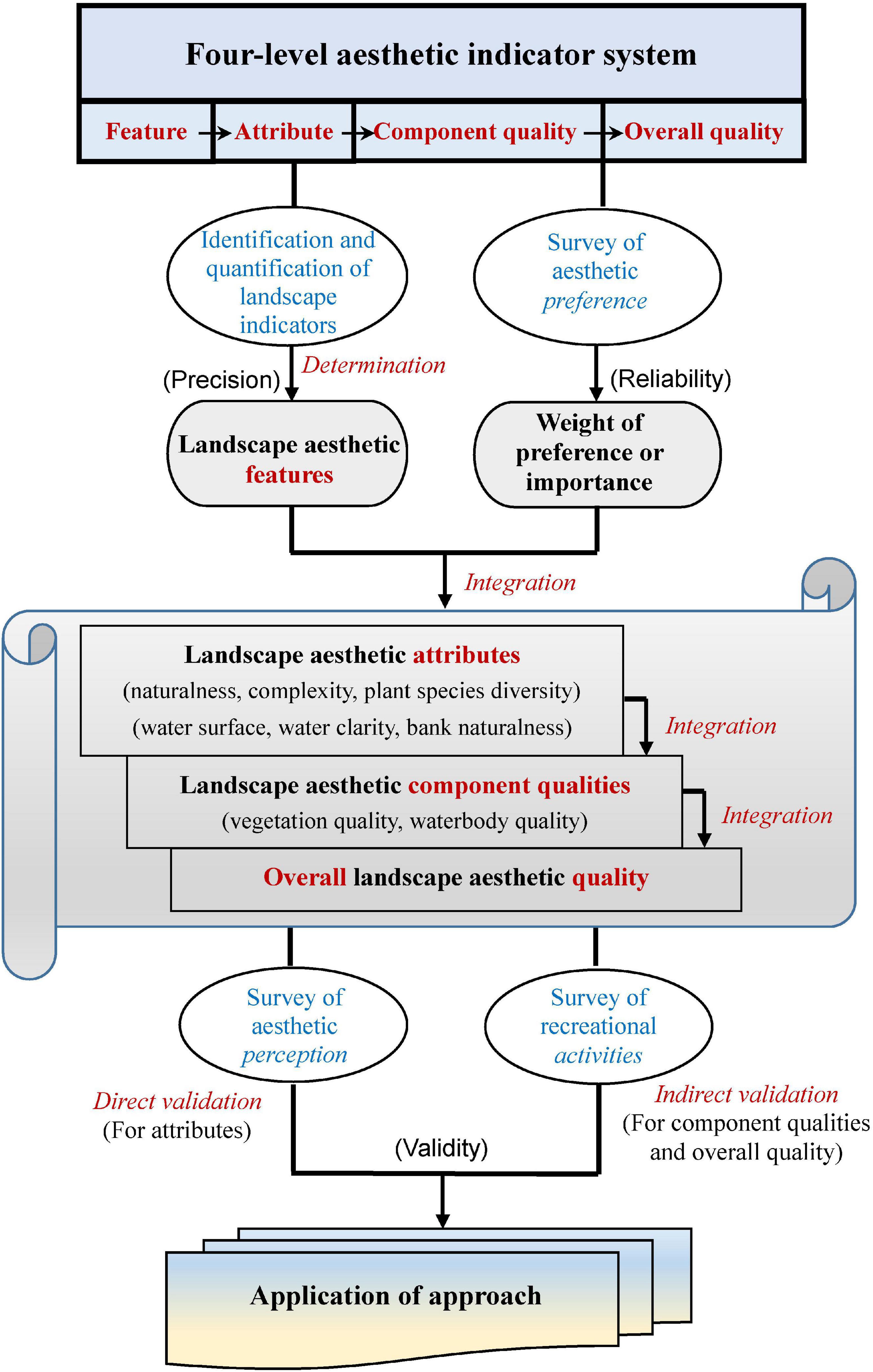
Figure 1. Comprehensive approach to aesthetic quality assessment of urban landscapes. The approach is based on a four-level landscape aesthetic indicator system from feature to attribute to component quality to overall quality. The approach is to realise the determination (including identification and quantification) of landscape aesthetic features, integration of objective indicators and subjective preferences for the estimations of aesthetic attributes, component qualities and overall quality, and validation of the estimations by direct surveyed perceptions and indirect recreational activities.

Materials and Methods

Study Area

The Yongding River, which originates in the Guancen Mountains in Shanxi Province and passes through Inner Mongolia, Hebei Province, and the cities of Beijing and Tianjing to the Bohai Sea (Figure 2A), is 747 km long with a basin area of 4.7 × 10⁴ km². At 170 km, it is the longest river in Beijing, including 37 km in the plain area (Figure 2B), and was called the mother river of Beijing.

FIGURE 2

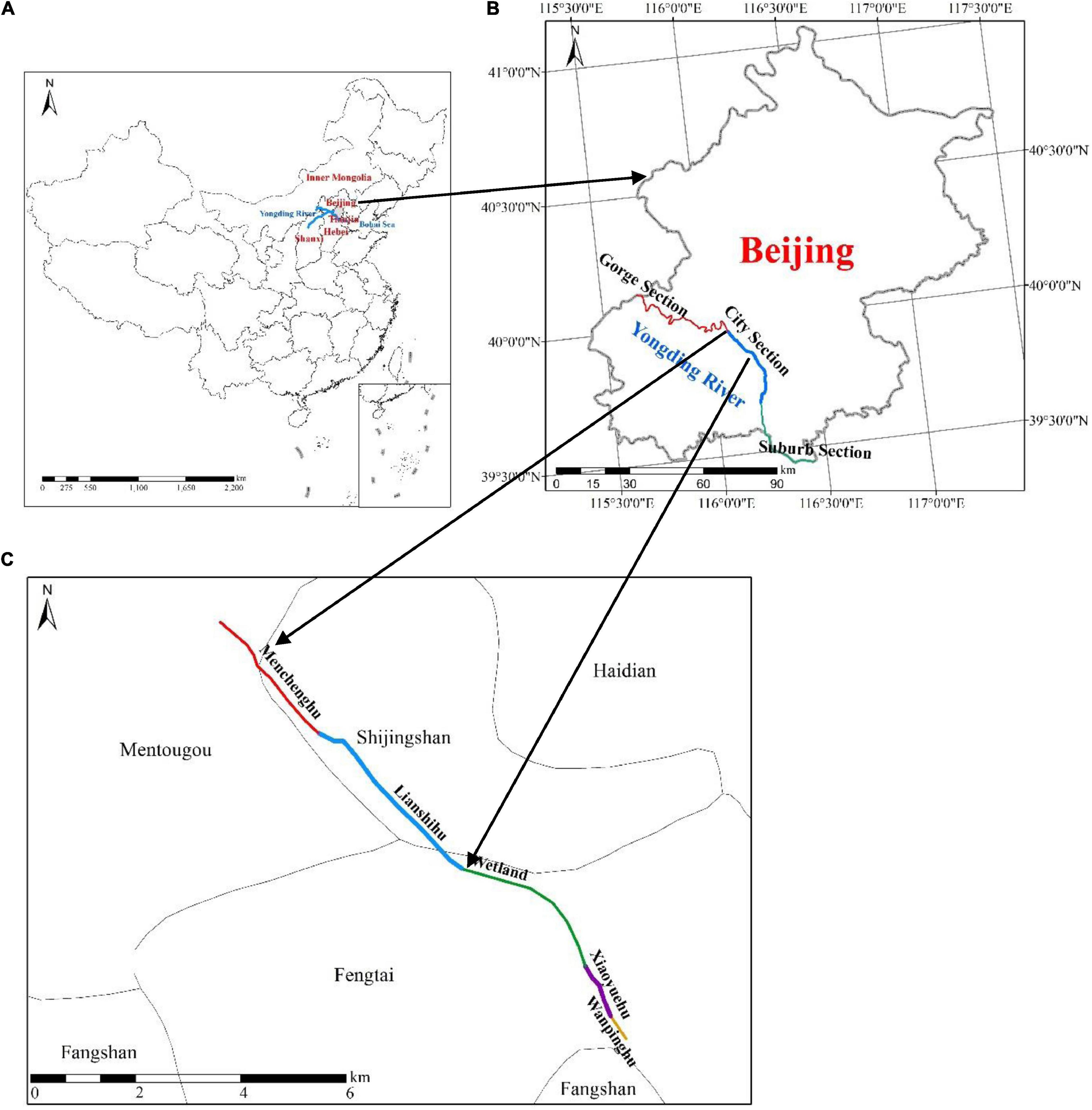
Figure 2. Location of study area Lianshihu Park including the Menchenghu and Lianshihu river subsections in the city section of Yongding River (C) of Beijing (B), China (A).

However, starting from the middle and late last century, the Yongding River was reconstructed to be mainly used as a drainage channel, and the increased water flow from agricultural fields and urban areas carried sediments and pollutants into the river with the fast pace of agriculture and urbanisation. This dramatically changed both the appearance and health of the river and riparian ecosystems, and even some river sections gradually dried up. The modification affected not only the nearby riparian buffers but also a large portion of Beijing’s water system. Since 2009, some restoration practices have been implemented on the riverbeds, banks, and buffers along the Menchenghu, Lianshihu, Xiaoyuehu, and Wanpinghu waterways in southwestern Beijing (Figure 2C). These included dredging the waterway, delivering more reclaimed water, forming multiple waterfalls horizontally across the water surface, meandering the riverbeds, increasing the earthen banks, and establishing the vegetated corridors along gently sloping zones (Zhu and Deng, 2012). Many trees, shrubs, and herbs were planted to form single or multi-layer green belts, although these were planted at similar times leading to a lack of biophysical variation among individuals within species.

Our study area is Lianshihu Park including the Menchenghu and Lianshihu river subsections in the city section, located in the east of the Mentougou District, neighbouring the southwest of the Shijingshan District and the north of the Fengtai District (Figure 2C), which are both large urban areas. The park was established after the restorations and leisure facilities were completed in September 2011. The total area of the park is 1.86 km², including 34.47% riparian buffer and 65.53% riverway. The park has become an important leisure space for local residents and visitors (Supplementary Appendix A).

Carrying with the great affections for the mother river of Beijing, many people have been counting on the improved environmental services and ecological health of the park after the restorations. We studied its services in improving water quality (Wang et al., 2015) and regulating surface runoff (Wang, 2015) and microclimate (Zheng and Zhang, 2016; Wang et al., 2020). However, its cultural services, especially its aesthetic values and recreation, which are the most directly correlated with human well-being, are still not systematically studied. The lack is a shortage when evaluating the restoring effects and offering advice for the future landscape design and planning.

Spatial Data and Field Survey of Land Cover Patches

A vector land cover map was created based on a four-band WorldView-2 image (0.5 m pixel resolution) for September 18, 2013 by on-screen digitising in ArcGIS 10.2. Image pre-processing, such as radiometric and atmospheric calibration and geometric rectification, was completed using ENVI 5.0 software. The vector map was converted to a raster layer with a 0.5 m spatial resolution. The land cover map was used to calculate some landscape metrics.

From the land cover map, 428 riparian patches with homogeneous land cover were identified. The interpreted type of each patch was tested through comparison with the field survey data in 2016. In the buffer, 369 vegetation patches accounted for 84.98% of the area. The mean vegetation patch size was 0.148 ± 0.216 ha, ranging from 0.001 to 2.058 ha. Paths, infrastructures, and buildings, which accounted for 11.38%, 2.12%, and 0.27% of the buffer, respectively, were also interpreted and tested. In this study, patch is the grain of landscape elements, the finest unit in which people can perceive spatial heterogeneity. A two-level patch classification system was developed, composed of five first-class and 32 second-class patch types (Supplementary Appendix B).

The entire riparian vegetation and corresponding river segments were divided into four landscapes (subareas A1, A2, A3, and A4), continuously located from north to south according to their vegetation and river conditions as well as infrastructure (Figure 3). The four subareas had the riverway length ranging from 1.58 to 1.93 km – the distance that most visitors could walk along the path in the park. It ensured that each subarea had an appropriate extent to accommodate visitors’ perceptions. The four subareas had small differences in vegetation area proportion of riparian buffer (80–89%). However, there were great differences in the abundance of riparian plants and vegetation patches, water surface size, and water quality (Table 1). Regarding riparian vegetation, A1 was similar to A4 while A2 was similar to A3; regarding river waterbody, A1 was similar to A2 while A3 was similar to A4. A4 had the highest plant abundance, most vegetation patches, and largest clear water area. The number of riparian vegetation patches in A4 was 22–46% higher than that in A2 and A3, and the water surface width in A4 was more than 220% higher than that in A1 and A2. By contrast, A2 had the lowest plant abundance and least vegetation patches and both A1 and A2 had the smallest water surface and most seriously contaminated waterbody. Moreover, compared with A1 and A2 with curving bank, A4 and A3 had straighter bank.

FIGURE 3

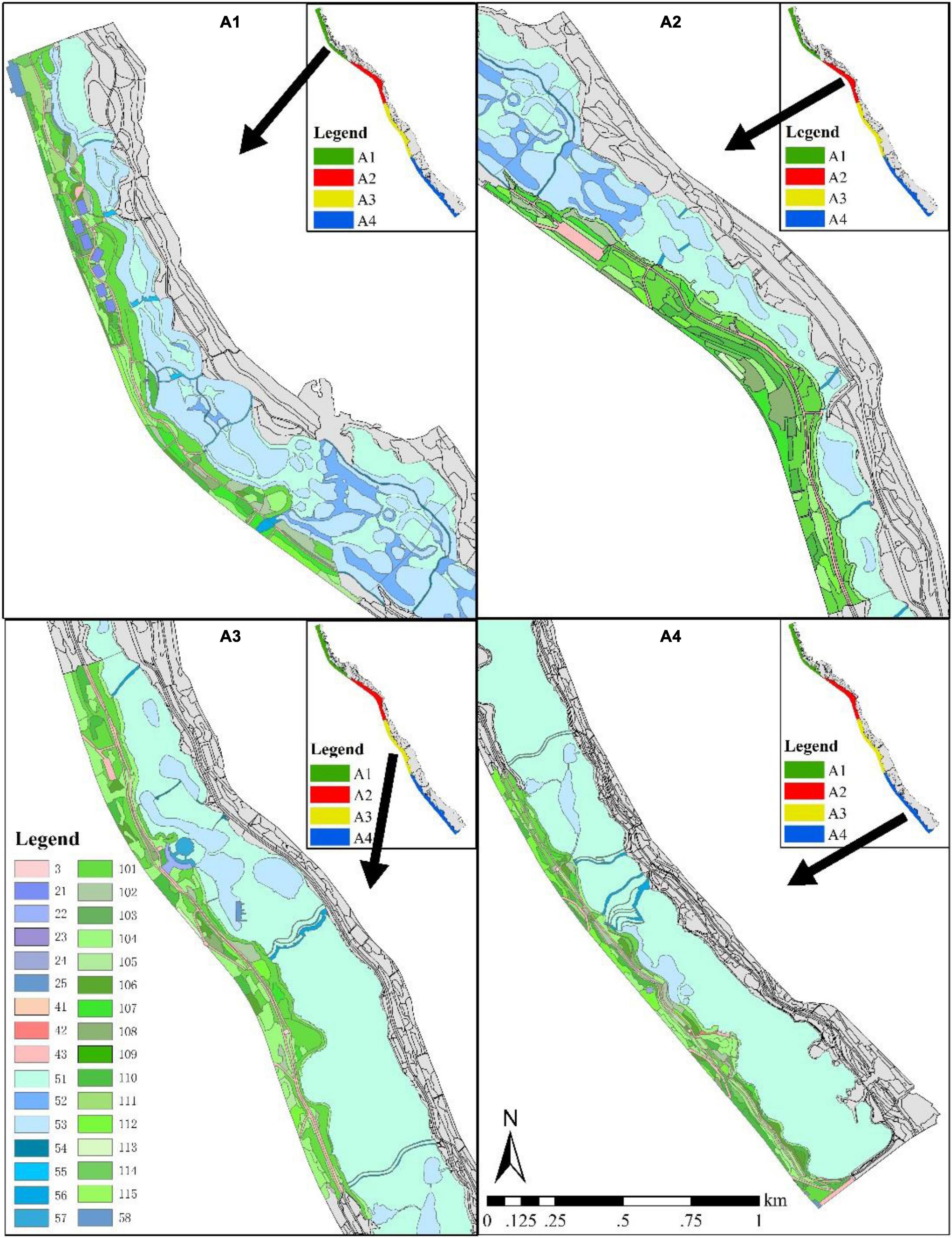
Figure 3. Four subareas along the Menchenghu and Lianshihu river subsections in Lianshihu Park. Legend indicates patch types whose meanings are given in Supplementary Appendix B.

TABLE 1

Table 1. Structural characteristics of the four subareas of Menchenghu and Lianshihu river subsections in Yongding River of Beijing.

Aesthetic Quality Assessment of Urban Landscapes

The proposed comprehensive approach was conducted on the assumption that landscape aesthetic preference and perception could be influenced by landscape elements. The approach covered the tasks ranging from determination and integration of aesthetic indicators to their validation (Figure 1).

Determination and Integration of Landscape Aesthetic Indicators

The construction of landscape indicators is an essential step in aesthetic assessment. We developed a hierarchical structure of four levels involving landscape feature, attribute, component quality, and overall quality from the bottom up. The highest level is overall landscape aesthetic quality. Component qualities describe different aspects of quality, such as vegetation and waterbody, which are visually and ecologically sensitive. Component quality is determined by the attributes associated with vegetation or waterbody aesthetics, while the attributes, in turn, can be described using feature metrics (Table 2).

TABLE 2

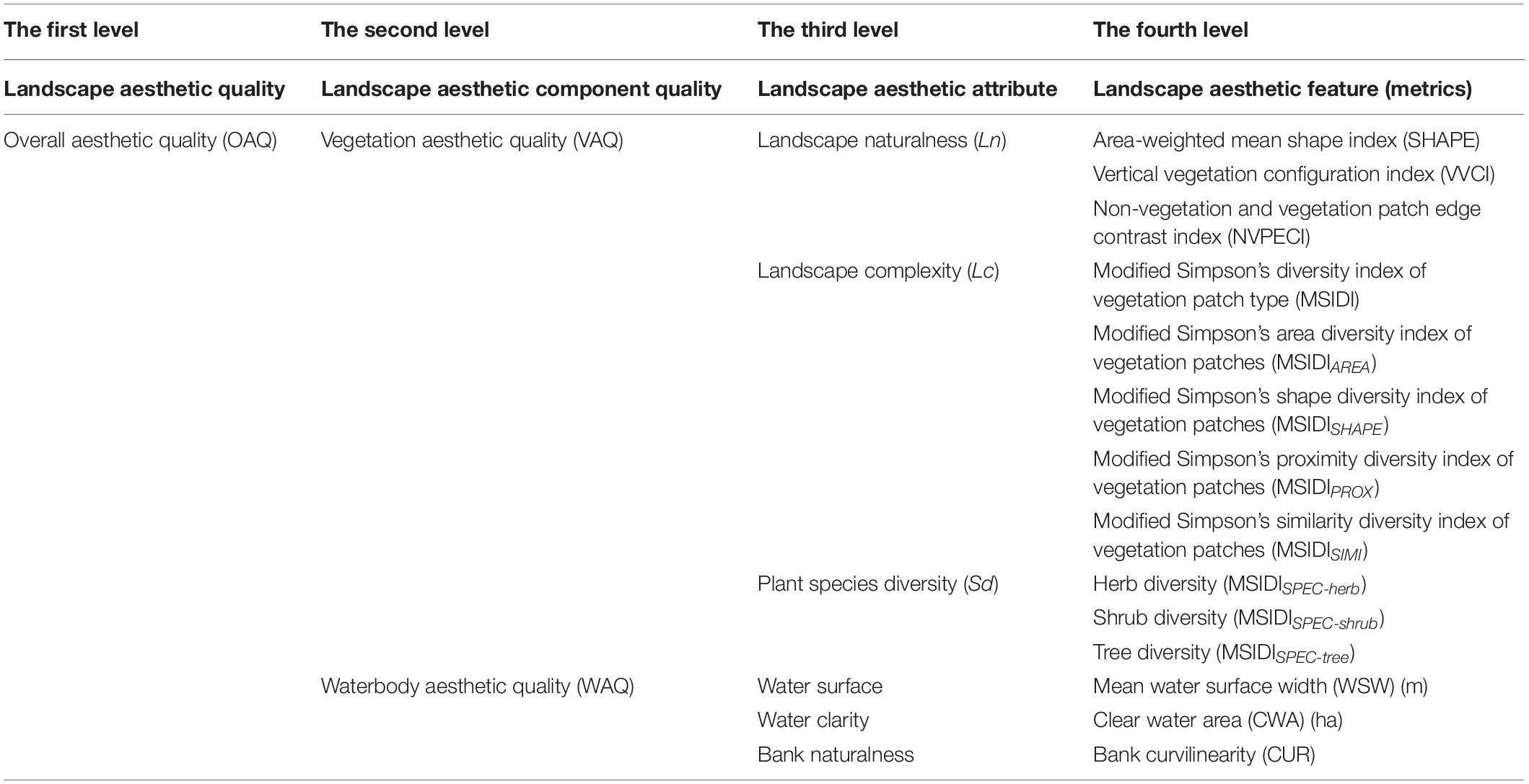
Table 2. Four levels of aesthetic indicator system of urban landscapes.

The inhabitants close to large urban areas are more likely to enjoy the environments with vegetation and waterbody, which have great difference in views and functions from the monotonous buildings where they more often live. Comparing with rural residents, these inhabitants tend to prefer more naturalised settings and varied views to relieve physiological and psychological stress and have higher leisure demands (Kaplan and Kaplan, 1989; Ryan, 1998; Hartig et al., 2003; Herzog et al., 2003). According to the literature and our interviews with visitors in the study area, landscape naturalness and complexity have been found to be the most key attributes that can enhance landscape preference (Kaplan and Kaplan, 1989; Lamb and Purcell, 1990; Real et al., 2000; Hands and Brown, 2002; Hagerhall et al., 2004; Palmer, 2004; Tveit et al., 2006; Schirpke et al., 2013; Sahraoui et al., 2016). However, few landscape studies were concerned with biodiversity that contains strong ecological meanings, because species cannot be readily identified from generally used land cover map, photos, or aerial images.

These aesthetic attributes present distinct perceptual and spatial characteristics. For example, greater naturalness means less human artefacts or disturbance and less rigid appearances; greater complexity creates richer vegetation patches or more varied patch configurations; and more plant species leads to higher vividness from various colours, leaf shapes, and tree structures (Kaplan and Kaplan, 1989; Parsons, 1991; Daniel, 2001). Moreover, these aesthetic attributes imply certain ecological functions or ecosystem services. For example, although naturalness is an ambiguous term in a landscape significantly influenced by humans, landscape patterns perceived as more natural are often perceived as more scenically beautiful and are often from more healthy ecosystems (Gobster et al., 2007).

In addition to vegetation, water is another landscape element that people clearly prefer (Kaplan and Kaplan, 1989; Tveit et al., 2006). Many studies have found that water area has a positive role on affective states (Kaltenborn and Bjerke, 2002; Faggi et al., 2011; Sahraoui et al., 2016). Several studies showed that aesthetic quality may also be affected by water movement or healthiness (Brown and Daniel, 1991; Cottet et al., 2013). People prefer naturally meandering rivers, which can create a greater aesthetic pleasure than straightened ones (Kondolf, 2006; Kenwick et al., 2009). According to the literature, our interviews with visitors, and our observations of human activities along the river, the three most critical attributes, water surface, water clarity, and bank naturalness, were selected to indicate waterbody aesthetics in our study area (Table 2).

These third-level landscape attributes were indicated by the fourth-level landscape features, which were quantified by metrics (Table 2). We developed new or used existing landscape-level metrics that include visual, perceptual, and spatial features and underlying ecological meanings. Given that the assessment method is intended to be generically applicable, most metrics should be able to be easily measured or estimated from land cover data or remote sensing data. Except for the mean water surface width (WSW), which were directly measured from images, we used or developed the metrics that integrate different characteristics. For example, diversity of vegetation patch areas (MSIDI_AREA) is the integration of the number of patch area classes (richness) and the proportional distribution of patch numbers among different patch area classes (evenness); clear water area (CWA) is the integration of total water area, contamination status, and water movement. Moreover, the selected metrics should be mutually independent to avoid considering their interrelationships when indicating an attribute.

In summary, we integrated the distinct landscape feature metrics to express different aspects of attributes. The derived attributes values were integrated to obtain the quality values for the two components, vegetation, and waterbody, which were further integrated to obtain a final value for the overall aesthetic quality (Figure 1).

Landscape Vegetation Aesthetics

(i) Landscape naturalness

When selecting the feature metrics that indicate landscape naturalness attribute, the two aspects, manufactured influence and human aesthetic preferences, were considered. Most deciduous trees, shrubs, and flowering herbs and all coniferous trees and shrubs in the study area were planted by design. There were no patches of completely wild vegetation; only a few native species and some wild forbs were sparsely interspersed or locally clumped within a patch. Consequently, perceived naturalness in an urban setting should be defined by the degree of deviation from natural appearance, rather than the presence or dominance of native plant species or management intensity in a more natural context (Tveit et al., 2006; Frank et al., 2013).

Moreover, perceived naturalness can be inconsistent with ecological naturalness (Daniel, 2001; Gobster et al., 2007). For example, disorderly growing wild forbs may not be considered scenically attractive by some visitors, although they may be more ecologically important than closely cropped lawns (such as in biodiversity and ecosystem resilience). Conversely, most urban landscapes with some exotic plants or orderly manicured green spaces represent slick-and-clean aesthetic, which may have negative effects on ecological conditions and human psychological functioning (Kenwick et al., 2009). To avoid these conflicts, we used or developed naturalness indicators in which aesthetic experiences and ecological benefits have complementary rather than contradictory implications for a landscape. Consequently, with these indicators, landscapes that are perceived as more natural are often ecologically robust (Gobster, 1999; Arriaza et al., 2004; Sahraoui et al., 2016).

A larger number of patches in a natural landscape have irregular contours than those in an artificial landscape. In natural forests, multi-layer vegetation, from herbs to underwood to canopy, and structurally complicated stands are common, Meanwhile, artificial forests are often dominated by single-layer and structurally simple stands. There is great clashing between a manufactured feature such as hardened paths and its natural background, and their visual contrasts in colour, texture, size, and shape greatly destroy the integrity of context (Hernández et al., 2004). Based on these analyses, we used an area-weighted mean patch shape index (SHAPE) in the spatial pattern analysis package FRAGSTATS 4.2 (McGarigal et al., 2012) and developed two new indices to quantify patch naturalness: vertical vegetation configuration index (VVCI) and non-vegetation and vegetation patch edge contrast index (NVPECI). SHAPE and NVPECI were calculated from the interpreted land cover map, while VVCI was from the field survey. SHAPE and VVCI at landscape level were lumped from the area-weighted mean indices for each patch (Supplementary Appendix C).

If the SHAPE value is low, visitors see more patches with simple geometric shapes. If the SHAPE value is high, they have a strong impression of naturalness due to the variety and complexity of patch shapes (de la Fuente de Val et al., 2006; Frank et al., 2013). VVCI indicates the whole complexity of vegetation layers from ground to canopy. A higher VVCI value indicates multiple vertical layers and more natural vegetation structure. NVPECI indicates the total contrast between vegetation and non-vegetation patches. A higher NVPECI means more infrastructures, buildings, or paths are adjacent to vegetation patches and greater non-vegetation patch density in a landscape dominated by vegetation. Once the path density or area of amenities crosses a threshold, what people perceive is the isolated vegetation patches that lack natural continuity. Hence, NVPECI can have a negative impact on landscape naturalness (Purcell and Lamb, 1998).

The values of SHAPE, VVCI, and NVPECI were normalised by dividing their respective maximums. An overall landscape naturalness (Ln) for each landscape was quantified using the model:

$Ln=w_{ln1}\cdot \text{SHAPE}+w_{ln2}\cdot \text{VVCI}-w_{ln3}\cdot \text{NVPECI}(1)$

where w_ln1, w_ln2, and w_ln3 are the weights of SHAPE, VVCI, and NVPECI in influencing Ln, respectively.

(ii) Landscape complexity

We selected the feature metrics that indicate landscape complexity attribute based on two aspects: composition and configuration of vegetation patches. Landscape composition associated with complexity may be quantified by patch richness (e.g., Palmer, 2004) and diversity index (e.g., Frank et al., 2013) to measure the variety of land cover or patch (Tveit et al., 2006). This study used a modified Simpson’s diversity index (MSIDI) in FRAGSTATS 4.2 (McGarigal et al., 2012) to measure the variety of vegetation patches. The vegetation patches were defined based on a two-level classification system including 15 groups (Supplementary Appendix B). The landscape with the higher MSIDI has a mixture of larger number of patch types (i.e., richer) with approximately equal area among different types (i.e., evener) (Palmer, 2004).

Based on MSIDI, we developed four modified Simpson’s diversity indices to measure the complexity of landscape configuration: diversity of patch area (MSIDI_AREA), diversity of patch shape (MSIDI_SHAPE), diversity of proximity between patches of the same type (MSIDI_PROX), and diversity of similarity to adjacent vegetation patches (MSIDI_SIMI) (Supplementary Appendix C). The more complex landscapes are those that have the higher diversity of patch area, shape, proximity, or similarity, meaning that the landscapes have both larger number of different classes of patch area, shape, proximity, or similarity (i.e., richer) and more equitable proportional distribution of patch numbers among different classes (i.e., evener).

Diversity of spatial pattern (especially area and shape) of single patches is the usual measurement of complexity (Tveit et al., 2006). However, diversity of spatial association among different patches is little mentioned. Proximity between patches of the same type and similarity to adjacent patches of the same and different types are important pattern characteristics that reflect spatial context of a patch in relation to its neighbours. We used the proximity index (PROX) and similarity index (SIMI) that can be calculated at patch level in FRAGSTATS 4.2 (McGarigal et al., 2012). PROX and SIMI can distinguish sparse distributions of small and insular patches from contiguous (or less fragmented) configurations with a complex cluster of larger and similar patches (Gustafson and Parker, 1992). A high diversity of proximity means there are obvious variations (high complexity) in the degree of patch isolation and the degree of fragmentation of the corresponding patch type, and a high diversity of similarity means there are obvious variations in the degree of patch isolation and the degree of contrast of all the patch types in a landscape mosaic. Within a landscape with high diversity of proximity, visitors may feel that the similar patches with different sizes occur at different locations. Within a landscape with a high diversity of similarity, visitors may notice the obvious variations in the vegetation contrast among the adjacent patches. That is, the adjacent plants that are very similar, similar, slightly contrasting, and sharply contrasting exist simultaneously.

The values of MSIDI, MSIDI_AREA, MSIDI_SHAPE, MSIDI_PROX, and MSIDI_SIMI were normalised by dividing their respective maximums. An overall landscape complexity (Lc) for each landscape was quantified using the model:

$\begin{array}{c}\hfill Lc=w_{lc1}\cdot \text{MSIDI}+w_{lc2}\cdot {\text{MSIDI}}_{AREA}+w_{lc3}\cdot {\text{MSIDI}}_{SHAPE}\hfill \\ \hfill +w_{lc4}\cdot {\text{MSIDI}}_{PROX}+w_{lc5}\cdot {\text{MSIDI}}_{SIMI}\hfill \end{array}(2)$

where w_lc1, w_lc2, w_lc3, w_lc4, and w_lc5 are, respectively, the weights of MSIDI, MSIDI_AREA, MSIDI_SHAPE, MSIDI_PROX, and MSIDI_SIMI in influencing Lc.

(iii) Plant species diversity

A modified Simpson’s species diversity index (MSIDI_SPEC) was developed, and MSIDI_SPEC–tree, MSIDI_SPEC–shrub, and MSIDI_SPEC–herb were used to measure the species diversity of tree, shrub, and herb layers, respectively, at the landscape level (Supplementary Appendix C). Simpson’s species diversity index is relatively less sensitive to richness than evenness and thus places more weight on the common species. By contrast, other indices (e.g., Shannon’s species diversity index) are more sensitive to richness than evenness and, thus, rare species have a disproportionately large influence on the magnitude of the index. Trees, shrubs, and herbs are one of urban green structure components. People’s perceived aesthetic of urban greenery is significantly correlated with estimates of biodiversity of these components (Gunnarsson et al., 2017). Separation of components (trees, shrubs, and herbs) with different plant functional traits (such as in life form) is crucial to make mechanistic understanding of various species’ contributions to aesthetics and ecosystem services (Lavorel et al., 2011; Andersson-Sköld et al., 2018).

To derive MSIDI_SPEC, we recorded plant species that occupied more than 1% of the patch area at any of the three vertical layers within each vegetation patch in August 2016. Spacing distances among plants were measured, from which the density and amount of each plant species were calculated (Supplementary Appendix C).

The values of MSIDI_SPEC–tree, MSIDI_SPEC–shrub, and MSIDI_SPEC–herb were normalised by dividing their respective maximums. An overall plant species diversity (Sd) for each landscape was quantified using the model:

$\begin{array}{c}\hfill Sd=w_{sd1}\cdot {\text{MSIDI}}_{SPEC\text{-}tree}+w_{sd2}\cdot {\text{MSIDI}}_{SPEC\text{-}shrub}\hfill \\ \hfill +w_{sd3}\cdot {\text{MSIDI}}_{SPEC\text{-}herb}\hfill \end{array}(3)$

where w_sd1, w_sd2, and w_sd3 are the importance degrees (weights) of variety at the tree, shrub, and herb species, respectively, in influencing Sd.

(iv) Landscape vegetation aesthetic quality

Although the three landscape attributes are presented independently, they have close links or overlaps and work together to form the totality of vegetation aesthetics. Given that Ln, Lc, and Sd had been normalised, the overall vegetation aesthetic quality (VAQ) for each landscape was quantified using the model:

$\text{VAQ}=w_{ln}\cdot Ln+w_{lc}\cdot Lc+w_{sd}\cdot Sd+\mathbf{\text{V}}\mathrm{\_}\mathbf{\text{INT}}(4)$

$\mathbf{\text{V}}\mathrm{\_}\mathbf{\text{INT}}=w_{\mathit{vin}\mathbf{2}}\cdot \mathbf{\text{V}}\mathrm{\_}{\mathbf{\text{INT}}}_{\mathbf{2}}+{\mathbf{\text{w}}}_{\mathbf{vin}3}\cdot \mathbf{\text{V}}\mathrm{\_}{\mathbf{\text{INT}}}_{\mathbf{3}}(5)$

where w_ln, w_lc, and w_sd are the weights of Ln, Lc, and Sd, respectively, in influencing VAQ. V_INT is the set of interaction among Ln, Lc, and Sd, probably including the interactions among any two (V_INT₂) or three (V_INT₃) attributes, whose corresponding weight sets influencing VAQ are w_vin2 and w_vin3, respectively.

Landscape Waterbody Aesthetics

We quantified waterbody aesthetic attributes from water surface, water clarity, and bank naturalness, which were measured using three metrics: mean water surface width (WSW), CWA, and bank curvilinearity (CUR).

From the interpreted WorldView-2 image, we divided the whole river way into multiple segments according to the riverbed width and fragmentation of waterbody from the amount, size, and distribution of islets and contaminated water areas. We measured the length and intermediate width of each segment using ArcGIS software. A length-weighted mean WSW was calculated for each subarea.

We derived turbidity (clear and slightly, more, or seriously contaminated) of the waterbody in each subarea from WorldView-2 image, which was tested through comparison with field survey data. We also observed the water movement (moving or static) in each subarea in mid-September 2016. River conditions were classified into five types: clear moving water, clear static water, clear but slightly contaminated static water, more contaminated static water, and seriously contaminated static water. These were given the weights of 0.9, 0.7, 0.5, 0.3, and –1.0, respectively. Finally, an area-weighted CWA was calculated for each subarea.

The banks of natural rivers in plains are mostly crooked, while artificial rivers often have straightened banks. Thus, rivers with a higher CUR present more natural bank. CUR was calculated by comparing the actual length of a bank and the length of straight bank with the same starting and ending points (Supplementary Appendix C).

The values of WSW, CWA, and CUR were normalised by dividing their respective maximums. The overall waterbody aesthetic quality (WAQ) for each landscape was quantified using the model:

$\text{WAQ}=w_{w1}\cdot \text{WSW}+w_{w2}\cdot \text{CWA}+w_{w3}\cdot \text{CUR}(6)$

where w_w1, w_w2, and w_w3 are, respectively, the weights of WSW, CWA, and CUR in influencing WAQ. The interactions among WSW, CWA, and CUR was not considered given that these three metrics were independent of each other.

Overall Landscape Aesthetic Quality

The overall aesthetic quality (OAQ) for each landscape was quantified using the model:

$\text{OAQ}=w_{c1}\cdot \text{VAQ}+w_{c2}\cdot \text{WAQ}(7)$

where w_c1 and w_c2 are, respectively, the weights of VAQ and WAQ in influencing OAQ. The interaction between VAQ and WAQ was not considered because the two components of vegetation and waterbody and their aesthetic attributes and features were strictly differed and their influences on OAQ were independent of each other.

In Equations 1–7, the quantifications of aesthetic indicators presented the integration of indicators, from features to integrated attributes to further integrated component qualities to finally integrated overall quality, by jointing objective indicators and subjective preferences.

Survey of Aesthetic Preference and Perception for Vegetation and Waterbody

Questionnaire-based on-site surveys of aesthetic preference and perception may provide a way to address the second question (integrating objective indicators and subjective preferences) and the third question (validating the estimated aesthetic indicators) proposed in Introduction section, respectively (Figure 4). While urban landscapes may have appreciable differences in scenic values, the correlations of preferred or perceived views with the landscape composition and configuration describing these views remain general. Typically, landscape differences are several orders of magnitude greater than the variations in observers’ judgements (Daniel, 2001; Palmer and Hoffman, 2001; Palmer, 2004). This is a basic assumption on which we can utilise survey data to assess aesthetic quality.

FIGURE 4

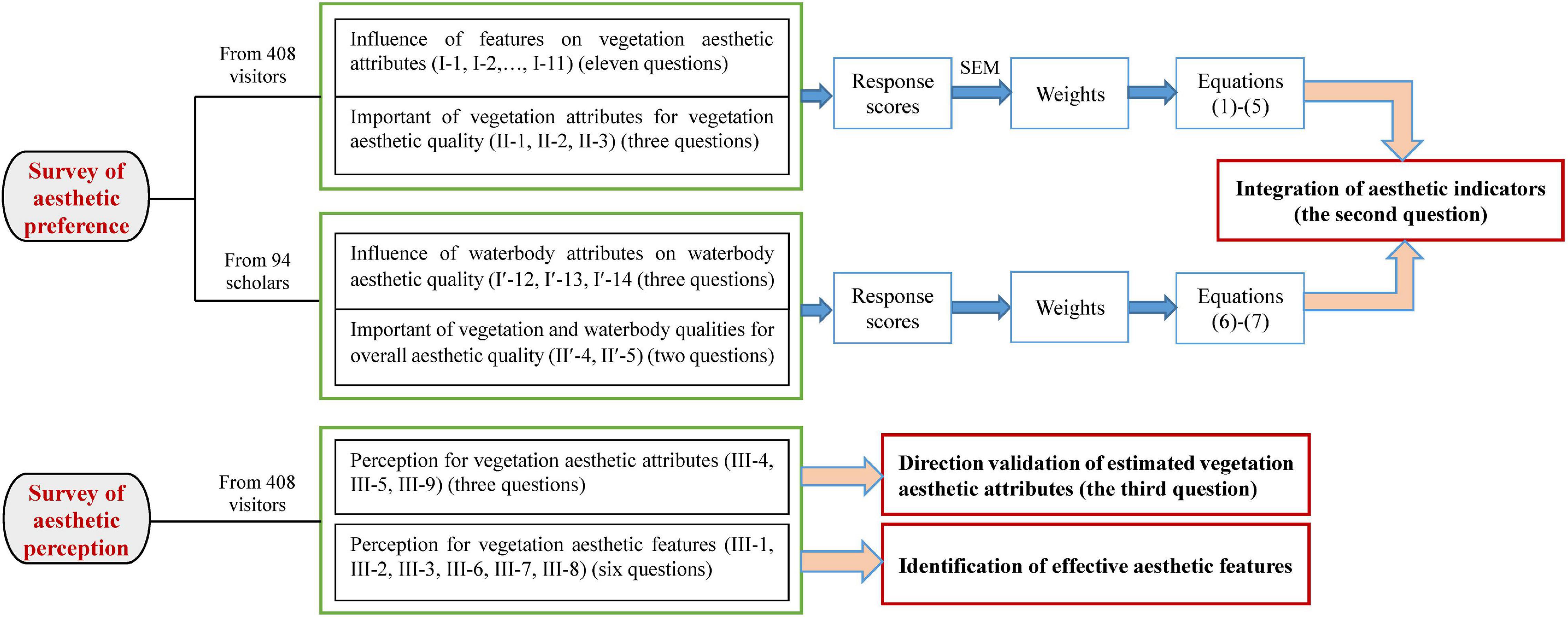
Figure 4. Survey of aesthetic preference and perception for vegetation and waterbody. SEM means structural equation modelling.

In our assessment, in order to obtain the six integrated predictors, aesthetic attributes (landscape naturalness, landscape complexity, and plant species diversity), vegetation and waterbody aesthetic qualities, and overall aesthetic quality, the weights in Equations 1–7 need to be estimated. This is associated with the second question proposed in the Introduction section. Although the estimations of these weights are based on objective landscape metrics, they depend more on subjective sentiments. Given that these weights cannot be measured directly, we conducted some preference surveys, from which the weights were estimated (Figure 4). The first category of survey (I-n) aimed for developing a detailed understanding of preferred settings, landscape elements, and spatial configurations. For each of the eleven questions, participants were asked to mark one of five boxes that most closely matched their preferences for the items about influence of a feature on its corresponding attribute. For example, “Influence of varying tree species (3–10 m) on plant species diversity” (I-1). The second category of survey (II-n) aimed for importance of landscape aesthetic attributes for quality. Three questions were asked to rate the extent to which a participant agreed with the importance of the three attributes (landscape naturalness, landscape complexity, and plant species diversity) for vegetation aesthetics. For these two categories of survey, a 5-point Likert scale method was used, offering five responses, “very much,” “quite a bit,” “somewhat,” “a little,” and “not at all,” given scores 5, 4, 3, 2, and 1, respectively (Supplementary Appendix D).

In our assessment, the validity of estimations of landscape attributes from Equations 1–3 need testing. This is associated with the third question proposed in Introduction section (Figure 4). Given that these response variables cannot be directly measured, we obtained the participants’ perceptual judgements for the attributes within the landscape where they were from the third category of survey (III-4, III-5, and III-9). Meanwhile, perceptual judgements of tree, shrub, and herb species diversity were asked (III-1, III-2, and III-3). In addition, whether a metrics (e.g., SHAPE, VVCI, and NVPECI) can effectively indicate an aesthetic attribute (e.g., naturalness) may also need to be tested (III-6, III-7, and III-8) by perceptual judgements. A scale of numbers (0–10) was set to rate the nine items. For example, “Please give a rating of landscape complexity within the subarea where you are” (III-5) (Supplementary Appendix D).

In the fourth category of survey (IV-n), participants were asked to respond based on the questions about demographics, trip characteristics, preference, and activity (Supplementary Appendix D). These questions provided the basis for analysing the connection between aesthetic perceptions and preferences and personal factors, although this study did not consider this issue.

However, we did not offer the questions associated with waterbody aesthetics in the visitor surveys and thus could not estimate the weights for waterbody and overall aesthetic quality in Equations 6, 7 based on the visitor surveys. To supplement the lack, we gathered the survey results from 94 Chinese scholars (including students) in the field of ecology or environment (Figure 4). Except for the questions associated with personal characteristics, five Likert scale questions were included to rate the influence of WSW, CWA, and CUR on waterbody aesthetic quality (I′-12, I′-13, and I′-14) and the importance of vegetation and waterbody for overall aesthetic quality (II′-4 and II′-5) (Supplementary Appendix D).

In summary, apart from the demographic questions, all the other questions refer to aesthetic preference or importance or perception. The preference surveys were to derive the weights of preference or importance and realise the integration of aesthetic indicators. The perception surveys were to validate the estimated indicators as well as evaluate the effectivity of some features (Figure 4).

On-site surveys to park visitors were conducted within all four subareas on both weekdays and weekends with sunny weather in August and September 2016. The participants were randomly selected, no matter who we met when we walked in the park. For the first and second categories of questions on preferences, the answers were open and not limited for any subarea. For the third category of questions on perceptions, the answers were specific for the subarea where the participants were. We sent out 600 questionnaire and finally gathered 510 effective and complete ones. We used 102 randomly chosen surveys for validation (about 25 ones for each subarea) and the remaining 408 ones for deriving the weights. Thus, the surveys for validation and deriving weights were independent of each other.

Weights of Landscape Aesthetic Preference or Importance

For Preference Survey From Visitors

Structural equation modelling (SEM) in the software Amos was used to estimate the weights in Equations 1–5. SEM is commonly justified to show the relations between unobserved latent variables and their observable indicators.

For our assessment, the three measurement models of SEM were constructed to test the hypothesis that aesthetic features influenced the corresponding aesthetic attributes that were the latent variables predicted in Equations 1–3 (Figure 5A). As the latent variable was landscape naturalness, the observed variables were the influence of irregular and varied vegetation patch shapes, the influence of multi-layer and structurally complicated vertical vegetation configuration, and the influence of number and arrangement of roads around vegetation patches on naturalness. As the latent variable was landscape complexity, the observed variables were the influences of diversity of vegetation patch types, area, shape, proximity of vegetation patches of the same type, and similarity or contrast to adjacent vegetation patches on complexity. As the latent variable was plant species diversity, the observed variables were the influences of varying tree, shrub, and herb species on total species diversity. The SEM inputs of observed variables were the 408 response scores for aesthetic preferences for landscape features from the first category of survey (I-n in Supplementary Appendix D).

FIGURE 5

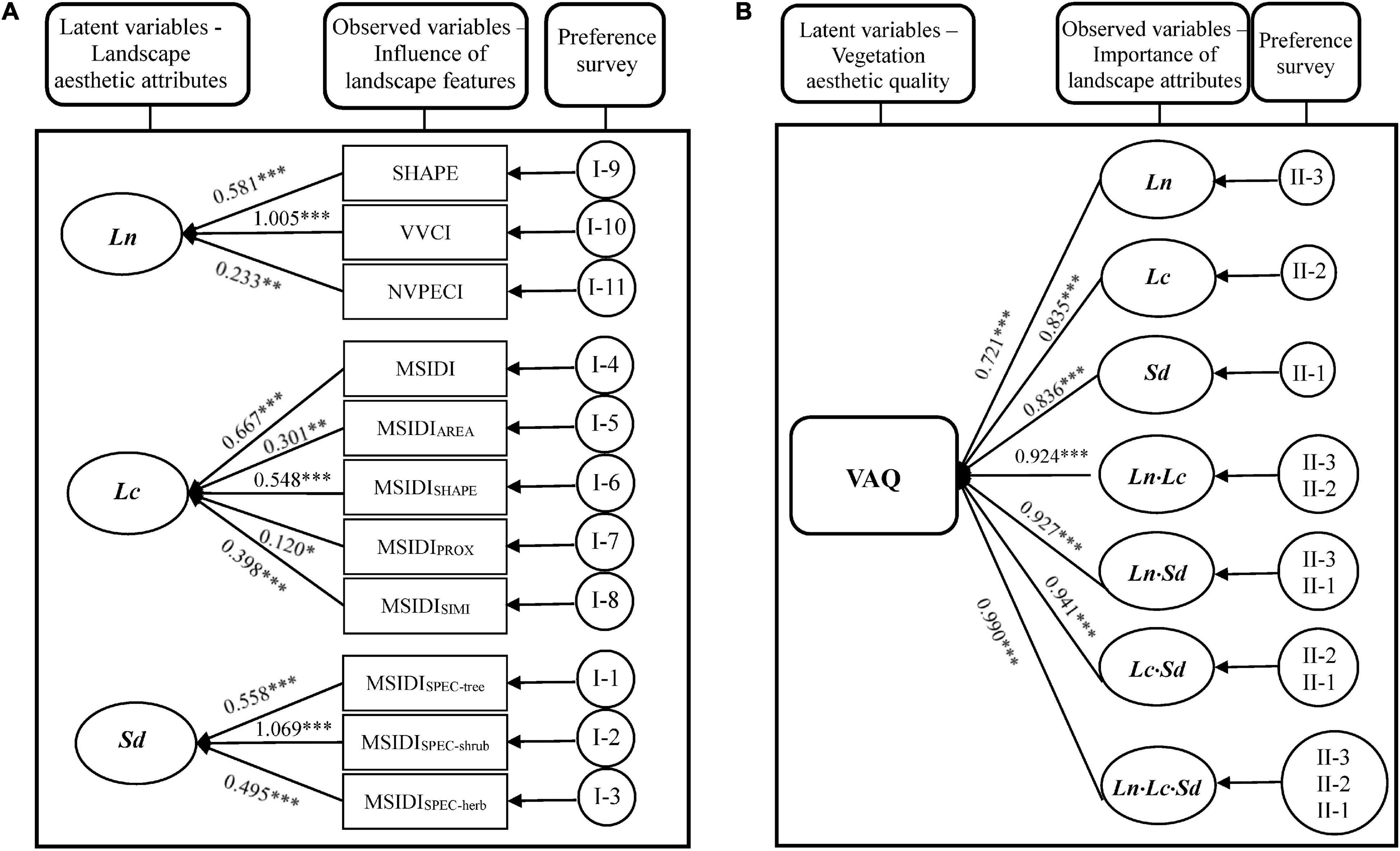
Figure 5. Path coefficients in the structural equation modelling: (A) to relate the landscape aesthetic attributes [landscape naturalness (Ln), landscape complexity (Lc), and plant species diversity (Sd)] to landscape features based on the surveyed aesthetic preferences for features; (B) to relate the vegetation aesthetic quality (VAQ) to landscape attributes based on the surveyed importance of attributes. The meanings of landscape aesthetic features are shown in Table 2. Significance: *p < 0.05; ^**p < 0.005; ^***p < 0.001.

The fourth measurement model of SEM was constructed to test the hypothesis that aesthetic attributes and their interactions influenced vegetation aesthetic quality that was the latent variable predicted in Equations 4, 5 (Figure 5B). The observed variables were the importance of naturalness, complexity, plant species diversity, and their interactions for vegetation aesthetic quality. For the single observed variables, the SEM inputs were the 408 response scores for the importance from the second category of survey (II-n in Supplementary Appendix D). For the interaction observed variables, the SEM inputs were the products of two or three response scores.

Model parameters were obtained through numerical maximisation via expectation–maximisation of a fit criterion provided by maximum likelihood estimation. Only the observed variables that were significantly correlated with a latent variable and met the requirements for model fits were good indicators of the latent variable. Given that the path coefficients are standardised versions of linear regression weights in the SEM method, in this study, they were used as the estimations of weights in Equations 1–5.

For Preference Survey From Scholars

We combined the 94 responses (from the 94 Chinese scholars in the field of ecology or environment in Section “Survey of Aesthetic Preference and Perception for Vegetation and Waterbody”) to calculate the proportions of scholars who gave different response scores, from which the weighted mean influence of water surface width, clear water area, and bank curvilinearity on waterbody aesthetic quality and importance of vegetation and waterbody aesthetic quality for overall aesthetic quality were estimated in Equations 6, 7.

Validation of Modelled Landscape Aesthetic Indicators

Direct Validation Based on Perception Surveys

Actually, it might not be the direct validation in a general sense because we could not directly measure the values of aesthetic attributes (landscape naturalness, landscape complexity, and plant species diversity) that fused multiple features. Here, direct validation meant direct comparisons between the estimations from Equations 1–3 and the surveyed third category of perception ratings from each landscape. As perception-based assessments have achieved generally accepted levels of precision and reliability (Lothian, 1999; Daniel, 2001; Palmer and Hoffman, 2001; Kearney et al., 2008; Frank et al., 2013), in this study, the perception ratings were used as references to validate the estimations.

Firstly, for the surveyed perception ratings of each aesthetic attribute, a Welch t test with 95% significance level was used to examine whether they were significantly different among the four subareas. Then, we observed whether the comparative relationships of the estimations among the four subareas were in accordance with those for the perception ratings. Further, if the regression model between the estimations and the perception ratings could explain more than 50% of the variance, then it was inferred that there was a close agreement between the two values.

Indirect Validation Based on Recreational Activities

Human recreational activities in a given area may largely indicate preferred scenes, as a decrease of scenic quality might reduce the attractiveness of the area and enjoyment of recreation (Schirpke et al., 2013). There is a correlation or synergy or overlap between recreation provision and aesthetics (Daniel et al., 2012; Casado-Arzuaga et al., 2014). It implies that some recreational activities may be used to indirectly validate aesthetic qualities.

We surveyed all the recreational activities in each subarea in the morning, afternoon, and evening, respectively, on both weekdays and weekends in mid-September 2017 when we walked along the paths. We recorded the locations and types of all activities, the number of participants, and the socio-demographic information. The results showed that the participants engaged in the following activities in decreasing order: strolling (37.23%), fishing (21.62%), sitting (19.08%), playing with water (8.09%), bicycling (7.05%), playing basketball (3.58%), jogging (1.50%), and others (1.85%).

Some of these recreational activities are correlated with aesthetics, whereas others may not. Hence, not all surveyed activities are considered as indirect validation of aesthetic quality. Specific activities (such as playing basketball and jogging) occurred only at specific sites (such as sports ground and running path) and not-fixed activities (such as bicycling) might occur in any landscape with a suitable path, so they rarely correlated with aesthetic quality in a site. Thus, only strolling, sitting, fishing, and playing with water were the concerned activities. In addition, we surveyed all the settings that might affect recreational activities in each subarea (Supplementary Appendix E).

Results

Vegetation Aesthetic Quality

Landscape Naturalness

The modelled results showed that the landscapes with higher plant abundance and more vegetation patches had higher landscape naturalness. VVCI had greater positive influence on naturalness than SHAPE and NVPECI. The weights were from the first category of preference surveys (I-9, I-10, and I-11 in Supplementary Appendix D) (Figure 5A).

$Ln=1.005\cdot \text{VVCI}+0.581\cdot \text{SHAPE}-0.233\cdot \text{NVPECI}(8)$

The subareas, ordered by decreasing modelled naturalness values, were A4 (0.733), A3 (0.688), A2 (0.672), and A1 (0.627) (Figure 6A). We compared these modelled values with the results from their perception surveys (III-9 in Supplementary Appendix D). The perceived naturalness values decreased across the subareas as follows: A1 (3.588 ± 0.957), A4 (3.441 ± 0.892), A3 (3.161 ± 1.068), and A2 (3.087 ± 0.848). A Welch t test showed that the perceived naturalness in A2 was significantly lower than that of A1 and A4, and there were no significant differences among other subareas. The correlation between the modelled and perceived naturalness was insignificant. However, we found that there was a close agreement between the modelled VVCI and the perceived naturalness and the regression model based on the four samples could explain 69.5% of the variance. The modelled VVCI values were 0.553 (A4), 0.520 (A1), 0.481 (A3), and 0.448 (A2) (Figure 6B).

FIGURE 6

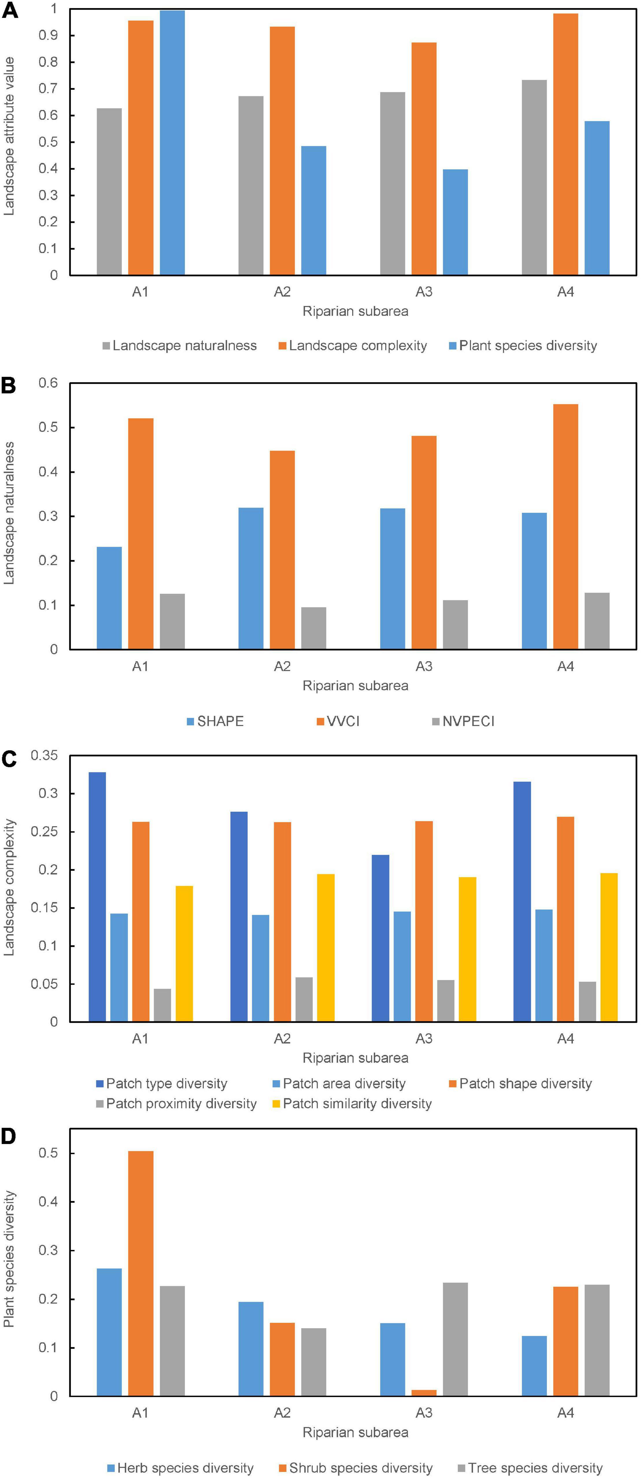
Figure 6. Modelled landscape attribute values (A) and feature values indicating landscape naturalness (B), landscape complexity (C), and plant species diversity (D) for the four subareas. SHAPE means patch shape index, VVCI means vertical vegetation configuration index, and NVPECI means non-vegetation and vegetation patch edge contrast index.

A4 had the most complicated vertical vegetation structure and complicated patch shapes and thus the greatest naturalness, despite having the most paths. A1 had the most regular patches and many infrastructures, while having a complicated vegetation structure. By contrast, A2 had the most complicated patch shapes and the least infrastructures, while having the simplest vegetation structure (Figure 6B). Therefore, when integrating the three features, A1 had the lowest naturalness, and when considering only the most significant feature (vegetation structure), it was A2 that had the lowest naturalness.

Landscape Complexity

The modelled results showed that the landscapes with more vegetation patches and a variety of patch types had higher landscape complexity. Diversity of patch type and shape had greater positive influence on complexity than diversity of patch similarity, area, and proximity. The weights were from the first category of preference surveys (I-4, I-5, I-6, I-7, and I-8 in Supplementary Appendix D) (Figure 5A).

$\begin{array}{c}\hfill Lc=0.667\cdot \text{MSIDI}+0.548\cdot {\text{MSIDI}}_{SHAPE}+0.398\cdot {\text{MSIDI}}_{SIMI}\hfill \\ \hfill +0.301\cdot {\text{MSIDI}}_{AREA}+0.120\cdot {\text{MSIDI}}_{PROX}\hfill \end{array}(9)$

The subareas, in decreasing order of modelled complexity values, were A4 (0.982), A1 (0.955), A2 (0.933), and A3 (0.874) (Figure 6A). We compared the modelled values with the results from their perception surveys (III-5 in Supplementary Appendix D). The perceived complexity values decreased across the subareas as follows: A1 (3.697 ± 0.847), A4 (3.525 ± 0.925), A3 (3.400 ± 1.102), and A2 (3.318 ± 0.894). The differences were not significant. The regression model between the modelled and perceived complexity could explain only 26.2% of the variance. However, when we involved only the two most significant metrics MSIDI and MSIDI_SHAPE, the regression model based on the four samples could explain 50.8% of the variance. The adjusted modelled complexity values were 0.591 (A1), 0.585 (A4), 0.539 (A2), and 0.484 (A3).

A4 had many vegetation patch types and the greatest variations in patch area, shape, and similarity, and thus the greatest complexity. A1 had the most patch types, which resulted in the greater complexity, although it had the least variation in patch configuration. By contrast, A3 had the lowest complexity, largely because it had the fewest patch types (Figure 6C).

Plant Species Diversity

The modelled results showed that the landscapes with more vegetation patches and a variety of patch types had higher plant species diversity. Shrub types had greater positive influence on species diversity than tree and herb types. The weights were from the first category of preference surveys (I-1, I-2, and I-3 in Supplementary Appendix D) (Figure 5A).

$\begin{array}{c}\hfill Sd=1.069\cdot {\text{MSIDI}}_{SPEC\text{-}shrub}+0.558\cdot {\text{MSIDI}}_{SPEC\text{-}tree}\hfill \\ \hfill +0.495\cdot {\text{MSIDI}}_{SPEC\text{-}herb}\hfill \end{array}(10)$

The subareas, in decreasing order of modelled plant species diversity values, were A1 (0.993), A4 (0.579), A2 (0.485), and A3 (0.397) (Figure 6A). We compared the modelled plant species diversity values with the results from their perception surveys (III-4 in Supplementary Appendix D). The perceived diversity values decreased across the subareas as follows: A1 (3.813 ± 0.859), A3 (3.484 ± 1.061), A4 (3.203 ± 0.983), and A2 (3.130 ± 0.694). A Welch t test showed that A1 had significantly higher diversity than the other subareas; there were no significant differences among A2, A3, and A4. The comparative relationships of the modelled diversity values from Equation 10 among the four subareas were almost in accordance with the perceived values. The regression model based on the four samples could explain 53.8% of the variance.

A1 had the most shrub and herb species and many tree species, and thus the greatest diversity, while A3 had the fewest shrub species and not many herb species, and thus the smallest diversity. A2 and A4 both had the medium shrub species, A2 had some herb species but the fewest tree species, and A4 had many tree species but the fewest herb species, and thus both the medium diversity (Figure 6D).

Vegetation Aesthetic Quality

The modelled results showed that the landscapes with higher plant abundance, more vegetation patches, and more patch types (A1 and A4) had the higher vegetation aesthetic quality. Both the single attributes (Sd, Lc, and Ln) and their interactions had strong influence on vegetation aesthetic quality. The weights were from the second category of importance surveys (II-1, II-2, and II-3 in Supplementary Appendix D) (Figure 5B).

$\begin{array}{c}\hfill \text{VAQ}=0.836\cdot Sd+0.835\cdot Lc+0.721\cdot Ln+0.941\cdot Lc\cdot Sd\hfill \\ \hfill +0.927\cdot Ln\cdot Sd+0.924\cdot Ln\cdot Lc+0.990\cdot Ln\cdot Lc\cdot Sd\hfill \end{array}(11)$

The subareas, ordered by decreasing modelled vegetation aesthetic quality values, were A1 (0.760), A4 (0.622), A2 (0.531), and A3 (0.474) (Figure 7A). A1 and A4 always had the higher quality than A2 and A3, even if landscape naturalness was indicated only by VVCI. There was a significant and linear regression relationship between the landscape metrics-based (modelled) and perception survey-based VVCI, landscape complexity, MSIDI_SPEC–herb, MSIDI_SPEC–shrub, MSIDI_SPEC–tree, and plant species diversity for all the subareas (r² = 0.242, p = 0.015) (Figure 8A). The significance greatly increased when MSIDI_SPEC–herb was not considered (r² = 0.417, p = 0.002) (Figure 8B).

FIGURE 7

Figure 7. Modelled waterbody aesthetic quality (WAQ), vegetation aesthetic quality (VAQ), and overall aesthetic quality (OAQ) (A) and feature values indicating WAQ (B) for the four subareas. VAQ_VVCI and OAQ_VVCI mean the VAQ and OAQ values based on just vertical vegetation configuration index (VVCI).

FIGURE 8

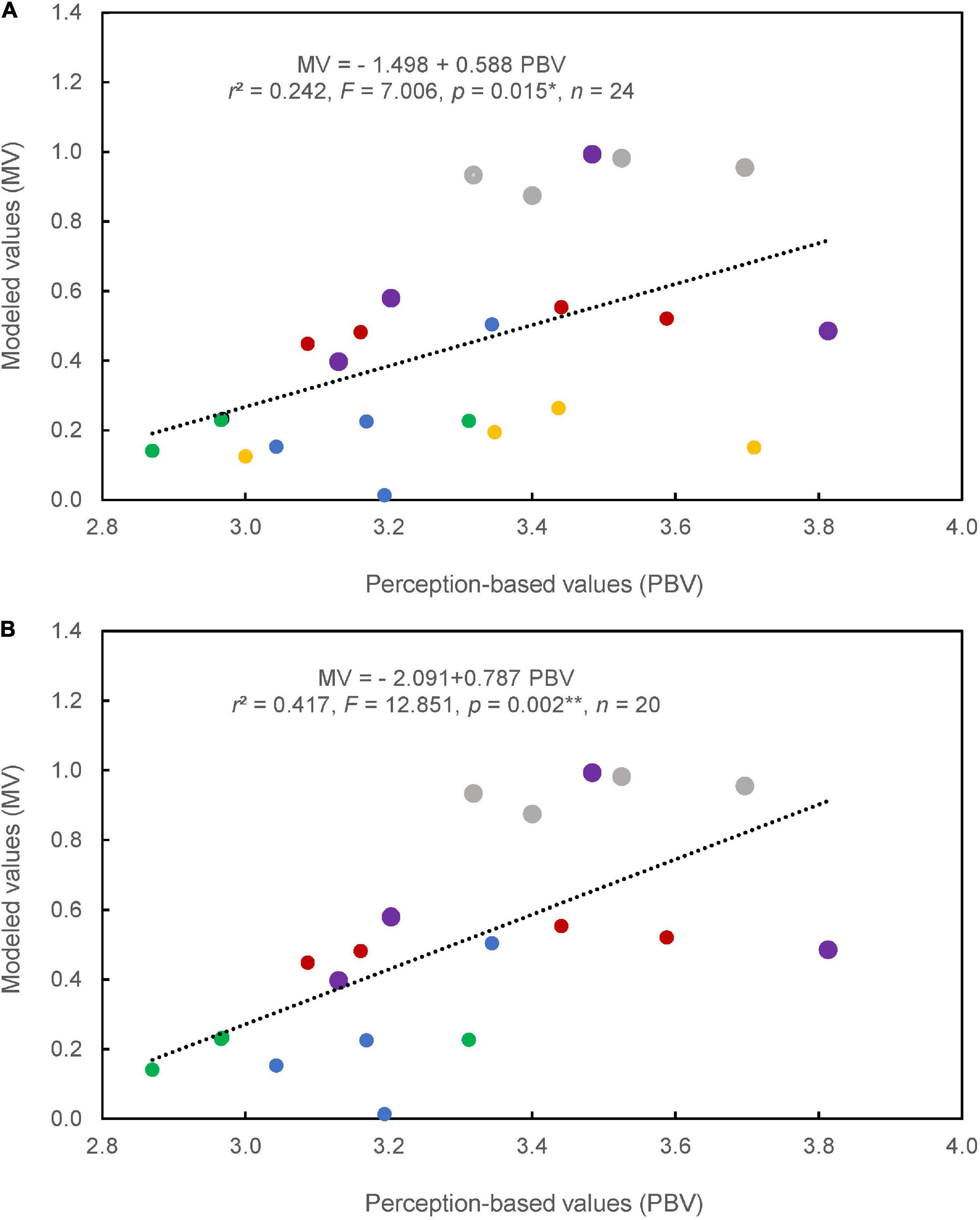
Figure 8. Relationship between modelled and perception-based values of herb (orange), shrub (blue), tree (green), and total plant species diversity (purple), landscape complexity (grey), and landscape naturalness (vertical vegetation configuration index, red) for the four subareas. Herb species diversity is included (A) and excluded (B), respectively.

Waterbody Aesthetic Quality

The modelled results showed that the landscapes with clearer water and larger water surface (A4 and A3) had the higher waterbody aesthetic quality. Clear water area and water surface width had greater positive influence on waterbody aesthetic quality than bank curvilinearity. The weights were from the preference scores given by the surveyed scholars (I′-12, I′-13, and I′-14 in Supplementary Appendix D).

$\text{WAQ}=0.588\cdot \text{CWA}+0.310\cdot \text{WSW}+0.102\cdot \text{CUR}(12)$

The subareas, ordered by decreasing modelled waterbody aesthetic quality values, were A4 (0.903), A3 (0.574), A2 (0.227), and A1 (0.190) (Figure 7A). Water surface width and clear water area could adequately account for these differences (Figure 7B). A1 and A2 had the narrowest water surface interspersed with some bare riverbed, averaging not more than 70 m, and they had a 16–20% seriously contaminated water area. A3 and A4 had the much wider water surfaces, averaging 162.62 and 218.82 m, respectively, and they had very large clear water area, just slightly contaminated at the riversides (Table 1).

However, the great bank curvilinearity in A1 and A2 (Figure 7B) did not significantly increase the total waterbody aesthetic quality (Figure 7A). One reason is that people might seldom concern whether the bank was meandering so much (with the lowest weight in Equation 12 from the preference surveys). Another possible reason is that bank curvilinearity was observable at the broad scale, and linear banks restricted the viewshed of most visitors.

Overall Aesthetic Quality

The modelled results showed that A4 had the highest aesthetic quality from both the highest plant abundance, the most vegetation patches, and more vegetation patch types (thus higher vegetation aesthetic quality), and the clearest water and the largest water surface (thus higher waterbody aesthetic quality). A2 had the lowest quality from both the secondly lowest vegetation and waterbody quality. A3 and A1 had the intermediate quality from either the higher waterbody quality while the lowest vegetation quality or the highest vegetation quality while the lowest waterbody quality (Figure 7A). The component that best explained overall aesthetic quality was vegetation, while waterbody had approximate contribution. The weights were from the importance scores given by the surveyed scholars (II′-4 and II′-5 in Supplementary Appendix D).

$\text{OAQ}=0.532\cdot \mathrm{VAQ}+0.468\text{⋅WAQ}(13)$

Strolling and sitting, the most frequent activities within the riparian vegetation buffer, occurred most in the subareas with higher vegetation aesthetic quality, which were A4 and A1 (Figures 7A, 9). In these subareas, visitors could enjoy varied or structurally complicated plants and colourful flowers (Figures 6B–D) when walking along paths, and they could spend much time under trees or near flowers. Therefore, there was a good match between modelled vegetation aesthetic quality values and surveyed buffer recreational activities.

FIGURE 9

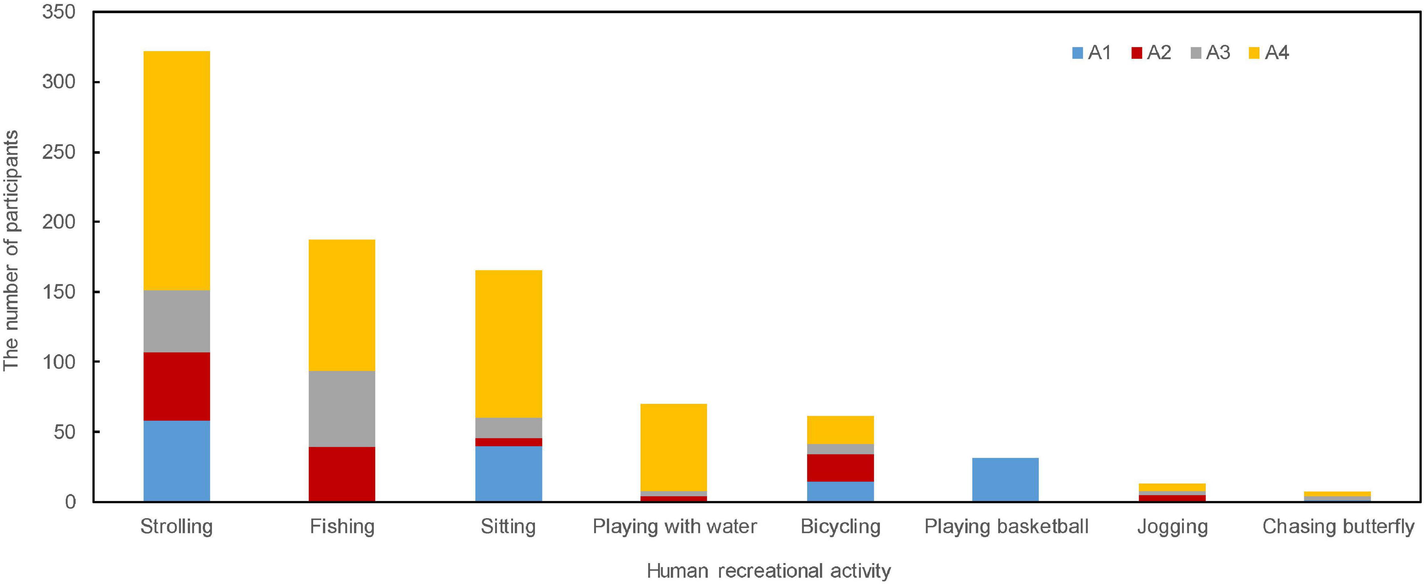
Figure 9. The number of participants engaged in recreational activities in the four subareas.

Fishing and playing with water, the most frequent water-based recreations at the riverside, occurred more in the subareas with higher waterbody aesthetic quality, which were A4 and A3 (Figures 7A, 9). In these subareas, visitors could enjoy playing with the open and clear water, and they could spend much time to play and catch more fishes at the riverside. By contrast, there was no water-based recreation that occurred in A1, which had the lowest waterbody aesthetic quality resulting from the narrowest water surface and worst water quality. Therefore, there was a good match between modelled waterbody aesthetic quality values and surveyed riverside recreational activities.

Discussion

Aesthetic value is a critical component of ecosystem cultural service, and aesthetic assessment can offer indispensable information for landscape design, planning, and management to improve human well-being. However, the current studies on determination, integration, and validation of landscape aesthetic indicators still cannot meet the requirement for precise, reliable, and valid aesthetic assessment. We find a comprehensive aesthetic assessment approach that shows promise for urban landscape research, taking into account both objective and subjective factors. The approach was applied to urban riparian landscapes as a case study. The results showed that vegetation and waterbody commonly contributed to overall aesthetic quality, accounting for 53 and 47%, respectively. The landscape with both higher plant abundance, more vegetation patches, and more patch types (exhibiting higher vegetation aesthetic quality) and clearer water and larger water surface (exhibiting higher waterbody aesthetic quality) had the higher overall aesthetic quality (such as A4), and vice versa (such as A2). If either vegetation (such as A1) or waterbody (such as A3) showed higher aesthetic quality, while another quality was lower, the landscape had the intermediate overall aesthetic quality. Vertical vegetation configuration had greater influence on landscape naturalness than patch shape and non-vegetation and vegetation patch edge contrast. Diversity of patch type and diversity of patch shape had greater influence on landscape complexity than diversity of similarity to adjacent vegetation patches, diversity of patch area, and diversity of proximity between patches of the same type. Shrub species diversity had greater influence on total plant species diversity than tree and herb species diversity. Clear water area and water surface width had greater influence on waterbody aesthetics than bank curvilinearity. These results were validated by comparing with the perceived naturalness, complexity, diversity, and by correlating with the main recreational activities. The case study demonstrated that the approach can address the three questions on determination, integration, and validation of landscape aesthetic indicators in some way and meet the generally required precision, reliability and validity of assessment systems, although some issues are still pending. Each of these issues is discussed below.

Determination of Landscape Aesthetic Indicators

Effectivity of Landscape Aesthetic Indicators

We used the landscape metrics that might be readily available. However, are their definitions effective to express some aesthetic meanings? For the landscape naturalness metrics (i.e., SHAPE, VVCI, and NVPECI), we compared the modelled patch-level metrics with the respondents’ perceptions for the naturalness of shape, vertical structure, and adjacent road of vegetation patches where they were (III-6, III-7, and III-8 in Supplementary Appendix D). The results, based on 102 patch data, showed that there were significant and linear correlations between all the three modelled metrics and the surveyed perception ratings (Figures 10A–C). Therefore, we concluded that the three metrics used in this study can effectively, at least to some extent, indicate features of naturalness.

FIGURE 10

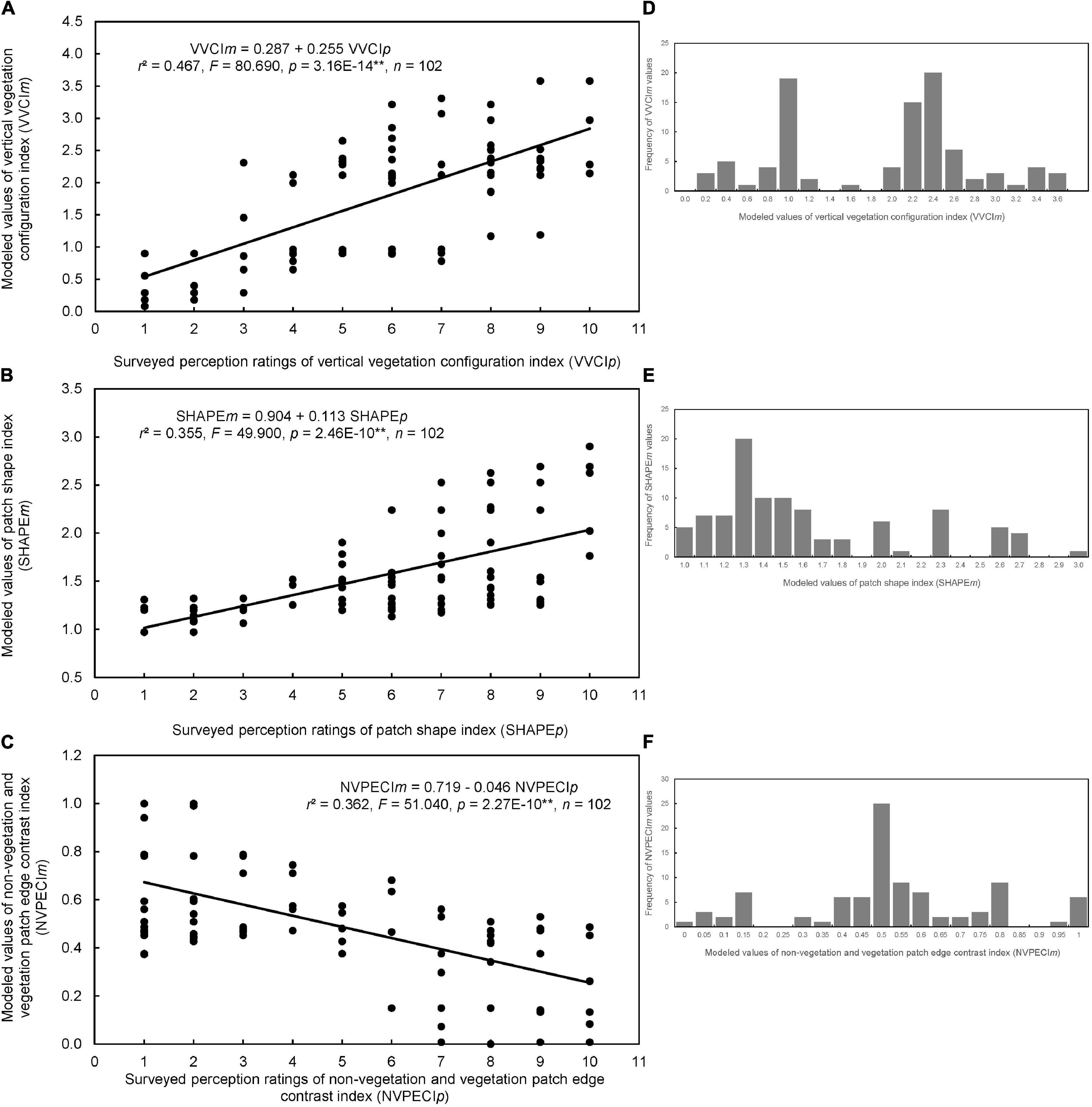
Figure 10. Relationships between modelled values of patch vertical vegetation configuration index (VVCIm) (A), patch shape index (SHAPEm) (B), and non-vegetation and vegetation patch edge contrast index (NVPECIm) (C) and surveyed perception ratings of naturalness of these patch indices (VVCIp, SHAPEp, and NVPECIp), respectively. Frequencies of VVCIm (D), SHAPEm (E), and NVPECIm (F) for the 102 perceived patches are also shown.

However, we found that not all the single metrics that were effective in indicating patch aesthetic features could be integrated to effectively indicate landscape aesthetic attribute. For example, in this study, the naturalness indicators initially modelled within a patch (though eventually integrated at landscape scale), such as VVCI, might be more effective than others, such as SHAPE and NVPECI. One reason might be perspective of observers for certain feature (Palmer, 2004). Most visitors perceived naturalness through vegetation conditions within a patch when they sat near trees or strolled along the path. By contrast, patch shape and patch edge contrast might not be legibly perceived via the observer’s interpretation of immediate surroundings (Kaplan and Kaplan, 1989). Another reason might be the degree that these feature values can be differentiated. Most observed patches (68.4%) had regular shapes with SHAPE from 1.0 to 1.6 (Figure 10E), and most (57.6%) had intermediate patch edge contrasts with NVPECI ranging from 0.4 to 0.6 (Figure 10F). By contrast to the more dominant distribution of SHAPE and NVPECI, VVCI had more even distribution, mainly ranging from 0.8–1.6 (36.2%) to 2.0–2.6 (48.9%) (Figure 10D). Approximate patch shapes and edge contrasts increased the difficulty in accurately differing them. Hence, SHAPE and NVPEVI did not relate to perception ratings as significantly as did VVCI (Figures 10A–C). That was one of the reasons why there was a much closer agreement between the modelled landscape naturalness values and the perception assessments when replacing landscape naturalness (Ln) (integrating VVCI, SHAPE, and NVPECI) with landscape-level VVCI. In summary, in our assessment, the single landscape metrics VVCI, SHAPE, and NVPECI themselves were all effective in expressing their distinct naturalness features, but VVCI was more effective in indicating naturalness attribute.

We also found that there was a much closer agreement between the modelled landscape complexity values and the perception assessments when replacing landscape complexity (integrating MSIDI, MSIDI_AREA, MSIDI_SHAPE, MSIDI_PROX, and MSIDI_SIMI) with adjusted landscape complexity (integrating MSIDI and MSIDI_SHAPE). Given that MSIDI and MSIDI_SHAPE contributed most to landscape complexity (Equation 9) and have been most widely used (e.g., Palmer, 2004; de la Fuente de Val et al., 2006; Tveit et al., 2006; Frank et al., 2013), this reduction was also reasonable.

Except for the total plant species diversity, we also compared the modelled diversity values for different plant components (herb, shrub, and tree) (Figure 6D) with the results from their respective perception surveys (III-1, III-2, and III-3 in Supplementary Appendix D). They had a certain degree of agreement, especially for the subareas with the highest or lowest modelled values. For example, A4 had the lowest modelled herb diversity; a Welch t test showed that A4 had significantly lower perceived herb diversity (3.000 ± 1.025) than the other subareas (3.348 ± 0.714–3.710 ± 0.938). A1 had the highest modelled shrub diversity; A1 had higher perceived shrub diversity (3.344 ± 0.865) than the other subareas (3.043 ± 0.928–3.194 ± 0.946), but not significantly so. A2 had the lowest modelled tree diversity; A2 had lower perceived tree diversity (2.870 ± 0.815) than the other subareas (2.966 ± 0.951–3.313 ± 1.148), to a significant degree in some cases. In summary, in our assessment, the classification of tree, shrub, and herb diversity was effective in expressing the diversity features from the distinct plant components, which was the critical basis of accurately modelling total plant species diversity.

Future Development of Landscape Aesthetic Indicators

Further analysis revealed that there is more to be developed regarding landscape feature metrics in urban areas not limited in the present study area. For example, for the present landscape naturalness metrics, VVCI was defined from a tree-shrub-herb structure. Further assessment could incorporate other vegetation structure, such as combinations of artificial and natural plants or native and alien plants or flowering and green leafy plants (Hands and Brown, 2002). In the present species diversity metrics, only plant species were considered, while further assessment could include animal species.

The spatial metrics, other than VVCI, reflected patterns within a two-dimensional space and did not investigate the potential effects of vertical factors (e.g., tree height, building height, or landform) on scenery and ecological processes. If these effects are significant, three-dimensional spatial metrics would be required.

In this study, landscape metrics were estimated for the entire landscapes. Local spatial heterogeneity can depend on the locations and composition of single vegetation patches within a viewshed and the spatial configuration of adjacent patches. Thus, aesthetic quality could be further assessed at multiple scales, from patch to neighbourhood to landscape (Daniel, 2001; Palmer and Hoffman, 2001). Moreover, spatial aesthetic quality can be estimated based on pixel-level metrics (Casado-Arzuaga et al., 2014).

Temporally, landscape mosaics may change over seasons or years. For instance, in vegetation colour or ephemeral herb species. Accounting for this requires a more dynamic aesthetic assessment, in contrast to the present static one (Tveit et al., 2006). However, identifying the aesthetic cues of spatiotemporal dynamics is a major challenge (Daniel, 2001).

It should be noted that our system utilises generic landscape indicators that are relevant for most urban green spaces and waterbody areas. For a specific environment, however, the assessment indicators should be adapted to the particular identity and processes. For example, the factors of architectural, historical, and cultural characteristics may have a critical influence on aesthetic quality (Sahraoui et al., 2016). Similarly, we ignore here the indicator, the proportion of vegetation, because vegetation area accounted for more than 80% in each subarea (Table 1). However, it may be an indispensable factor for many non-vegetation dominated landscapes (Palmer, 2004; Sahraoui et al., 2016).

Regarding waterbody aesthetic indicators, it will be interesting to select other factors such as bank composition (e.g., concrete, stone, brick, and soil) and view to the water and explore preferences for them (Kenwick et al., 2009). Water is given special attention in relation to coherence or harmony of scene in a landscape, and thus, potential visual indicators may include water presence and its spatial location and water colour (Tveit et al., 2006).

Integration of Objective Estimations and Subjective Preferences

In our models (Equations 1–5), to get final landscape aesthetic indicators, both landscaper metrics and their weights in influencing aesthetic indicators were considered. We derived the weights from visitors’ subjective preferences. Gathering feedback from visitors about their aesthetic preferences is important for better evaluating landscapes. In this study, human aesthetic preferences and their relations to landscape composition and configuration could be assumed to be relatively stable although landscape elements might vary with time and space. The reasonability of this assumption has been confirmed in many landscapes, especially in pleasant landscapes (Hagerhall, 2001; Kalivoda et al., 2014). Due to common human evolutionary history, there exist similar aesthetic preferences across cultures and personal differences (Palmer, 1997, 2004; Tveit et al., 2006; Jorgensen, 2011). On the other hand, the most respondents were local residents (69.3% within the range of 10 km around the park), which made it highly possible that they have the common socio-cultural surroundings and the relative consensus in aesthetic preferences. Moreover, a large number of independent respondents (408) greatly elevated the reliability of the derived weights. Therefore, our preference study could help to develop a more general understanding of subjective processes underlying aesthetic choices.

The Equations 1–5 showed how objective metrics and subjective preferences were integrated to obtain each landscape attribute and overall vegetation aesthetic quality. This integration is one of the advantages of our assessment by comparing with expert or landscape metrics-based (both dominant in objective component) or perception-based (dominant in subjective component) assessments. This integration fused objective features and subjective preferences (more general over time and space) rather than objective features and subjective perceptions (more specific at time and space) like in psychophysical assessment, which ensured the generality of conclusions and applicability for other landscapes.

However, there were still some drawbacks in deriving weights through preference surveys in this case study. For example, the survey samples and methods to estimate the weights of riparian vegetation aesthetic indicators are different from those to estimate the weights of river waterbody aesthetic indicators. The inconsistence might influence the assessment when integrating vegetation and waterbody aesthetics, although it will not influence their respective assessment. Therefore, in this study, the final overall aesthetic quality was more of a reference meaning. Further study will consider the mutual interaction between vegetation and waterbody aesthetics when their survey samples and methods are consistent.

Some feature indicators may be hardly understood by non-experts (Frank et al., 2013). For instance, visitors may understand variations in patch type, area, and shape. However, the concepts of proximity or similarity diversity may not be easily comprehended, which increases uncertainty. However, this uncertainty was moderated by the greatest contribution of MSIDI and MSIDI_SHAPE and the smallest contribution of MSIDI_PROX to landscape complexity (see Equation 9).

We did not differentiate the responses of local and non-local visitors. However, these groups may have different aesthetic preferences (Frank et al., 2013; Deng et al., 2017). Non-local visitors are often more sensitive to how the scenery differs from their previous living space, while local visitors may be accustomed to the scenery. Moreover, the lifestyles and habits formed in different environments may lead to different aesthetic preferences. If this were the case, the responses would need to be studied at group level.

Another set of factors that may be important to form aesthetic preferences are personal characteristics including age, gender, education, experiences, occupation, income, hobbies, and professional qualification (Van den Berg et al., 1998; Jorgensen, 2011; Kearney and Bradley, 2011; Sahraoui et al., 2016; Wang and Zhao, 2017). There might still be more or less variability among individual preferences even if under the similar socio-cultural surroundings and political and economic contexts (Kalivoda et al., 2014). We will examine the impacts of interpersonal differences on landscape aesthetic choices and experience in a future study.

Validation of Modelled Landscape Aesthetic Indicators

Direct Validation Based on Perception Surveys

Perception surveys were supposed to be applied for validating the modelled landscape attribute values. Comparing with viewing photos or other visual media, on-site observations and actual experiences of real multi-dimensional landscapes could improve the validity of assessments (Palmer, 2000). In this case study, the large number of observers (102) also greatly elevated the reliability of the subjective perceptual judgements.

We compared the relative relationships of the modelled landscape attribute values among the four riparian subareas with the participants’ perceptual judgements. We found that the approach could account for the detailed differences in visual characteristics among the discrete subareas, which were artificial landscapes with only slight differences in vegetation elements. For the landscapes with obviously different scenic features, the approach is expected to deliver more contrasting results. To confirm the expectation, a sample of urban landscapes with greater variability should be included.

However, this relative comparison is normally used with small sample size, when other quantitative methods are limited or statistics cannot successfully explain certain quantitative relationships. For example, in our case study, we found high correlations between perception-based and landscape metrics-based results of VVCI, adjusted landscape complexity, and plant species diversity in the four subareas, but their regression relationships based on the four samples were insignificant even though r² was as high as 0.695. Hence, taking into account the restricted regional context and the small sample size, we cannot confidently state that our modelled landscape attribute values do deliver reliable results. We suggest that future studies should test the applicability of aesthetic attributes in different landscapes.

The aesthetic indicator values obtained from perception surveys were assumed to be true, although the validation was constrained by the lack of consensus on the meaning of aesthetics and agreed-upon theories of visual landscape aesthetics (Daniel, 2001; Sahraoui et al., 2016), which is beyond the study. We discuss here several potential sources for the uncertainty of landscape perceptions.

1) Uncertainty of perception from landscape complexity

From the regression and correlation analysis, we found that the agreement between the modelled and perception-based landscape complexity was not as good as that for VVCI (indicating landscape naturalness) and plant species diversity. Landscape complexity is an abstract concept, and it is not easy to determine what landscape elements actually constitutes complexity and how these relate to aesthetic perceptions (Tveit et al., 2006). More importantly, landscape complexity must be obtained from the landscape as a whole, and some perceptions did come from an extensive view over the surrounding area, while other perceptions might come from a fixed viewpoint. The possible mismatch between observed scales and intrinsic scales increases the uncertainty (Palmer, 2004).

2) Uncertainty of perception from single landscape aesthetic feature

In this study, in addition to the three integrated landscape attributes, we assessed and validated single aesthetic features such as herb, shrub, and tree species diversity by comparing estimations with how they were perceived. However, the agreements here were not as strong as those for holistic landscape attribute (plant species diversity), except for high consistency in the subareas with the maximum or minimum values. The regression relationship in which MSIDI_SPEC–herb was one of the independent variables was less significant than when it was excluded (Figures 8A,B). Equation 10 also showed that in comparing with shrub and tree species, herb species made the smallest contribution to plant species diversity. Most visitors identified herb species without specific knowledge of species taxonomy, resulting in most subareas being perceived as having similar herb species diversity (Figure 6D), although actual diversity might differ greatly. The holistic judgement of landscape attributes (e.g., plant species diversity) can reduce the arbitrariness and uncertainty that comes from the perception of single features (e.g., MSIDI_SPEC–herb) (Hagerhall, 2001).

3) Uncertainty of perception from participants

Like the preference study, we did not differentiate the perceptions of local and non-local visitors and did not incorporate the influence of demographic factors on perceptions.

Indirect Validation Based on Recreational Activities

We did not make perception survey for overall vegetation and waterbody aesthetic quality, and thus could not directly validate them. They were indirectly validated based on the recreational activities correlated with vegetation and waterbody scenery, such as strolling, sitting, fishing, and playing with water. However, there were still other factors that might influence the potential relationships between aesthetic quality and recreational activities, even if we left out the activities that linked the factors beyond the aesthetic quality (such as playing basketball, jogging, and bicycling).

It seems that there is no close relationship between fishing and waterbody aesthetic quality, and fishing should be more affected by the seemingly more important factors (such as amount of fish). However, some hidden relationships can be found based on the direct linkage between amount of fish and water conditions (including water area and water quality) associated with waterbody aesthetics. Moreover, like other activities such as strolling, sitting, and playing with water, fishing was more of a kind of leisure activity to relax and enjoy rather than to acquire food in this park. Hence, it was surrounding environment and water conditions rather than amount of fish that was the most important factors to select fishing sites.

In some cases, it may be necessary to further differ short-time and long-time activities or identify purposes of activities when relating them with aesthetics. For example, what many seats beside paths offered was more of temporary resting rather than prolonged staying for chatting or playing. Only if an activity lasted for quite much time at a site can it be used to indicate its relationship with the site’s aesthetics, because it implies that the site and its surroundings can offer pleasant scenery, not just a temporary resting place. In some way, this resulted in more sitting while entertaining in A1 and A4 where there was more pleasant vegetation environment.

In some cases, it seems that some physical settings may play more important role than aesthetic quality in the occurrence of these activities (Casado-Arzuaga et al., 2014). If it were the case, the activity-based indirect validation will be not reliable. The existence of some settings (such as seats and fishing platform) does increases the chance of an activity (such as sitting and fishing). However, the existence or number of these settings may not be highly correlated with the occurrence of some activities. For example, A3 had about 34 more seats beside the paths than both A1 and A4 (Supplementary Appendix E), but more sitting in A4 and A1 than in A3 (Figure 9), because sitting occurred not only in seats but also on ground. Whether there was a seat was not as important as whether there was more tree shade. In both A4 and A1, large tree crowns (averaging 1.5 m width) provided more shades and comfortable microclimate. From the correlation analyses between the number of visitors sitting near trees and tree crown breadth (Pearson correlation coefficient R = 0.843), it showed that presence of large tree crowns made visitors significantly more likely to stay in the shades. Both A2 and A3 had small tree crowns (averaging 1.0 m width), and consequently far fewer visitors sat there in the hot summer. Moreover, A3 had the only fishing platform over the entire buffer (Table 1), but much more water-based recreations occurred in A4, where people fished or played with water on the trampled open spaces along the riverside rather than on a fishing platform. Therefore, in this study, it was vegetation and waterbody conditions (rather than physical settings) that were highly appreciated for recreational activities like sitting, fishing, and playing with water. In this sense, the activity-based indirect validation of aesthetic quality was reasonable and reliable.

Conclusion

We proposed a comprehensive approach for aesthetic quality assessment of urban landscapes to address the questions on determination, integration, and validation of landscape aesthetic indicators.

For the determination of quantitative landscape aesthetic indicators, a four-level system was developed, from the bottom features up to attributes, component qualities, and finally overall quality. The selected feature metrics could provide objective information on landscape visual and spatial features and ecological implications. In addition, they could account for the impact of landscape composition and configuration on aesthetic quality. However, the selection of metrics is open, and metrics should vary with study areas.

To obtain each integrated landscape aesthetic attribute and quality, we conducted questionnaire-based surveys for aesthetic preferences, from which the more general weights of each feature influencing corresponding attribute, the importance of each attribute for vegetation or waterbody quality, and the importance of each component for overall quality were derived. The approach implemented the joint of objective metrics and subjective preferences and thus addressed the question on the integration of aesthetic indicators. This joint is also one of the advantages of our approach comparing with expert-based or landscape metrics-based or perception-based assessment approaches.

In our case study for artificially restored adjacent riparian landscapes, we observed that landscape naturalness, landscape complexity, and plant species diversity as modelled by the integrated landscape metrics had high and positive correlations with perception-based aesthetic judgements from visitors. What is needed now is to conduct an extended study for other types of scenes in other geographic locations and socio-cultural contexts to assess these relationships. Moreover, the modelled vegetation and waterbody aesthetic quality values were able to explain main recreational activities within the vegetation buffer and at the riverside, respectively. These results validated the integrated aesthetic predictors and the comprehensive assessment approach.

In theory, the methodology is replicable and hence transferable to other frameworks that assess ecosystem cultural service. In practice, the approach is expected to extrapolate to other urban landscapes with some modifications in the future. The approach can be useful in establishing indicators to quantify, measure, and compare the current landscape aesthetic qualities and predict the effects of landscape design, planning, and management on aesthetic characters. Finally, the approach is open to criticism and improvement by peers.

Data Availability Statement

The raw data supporting the conclusions of this article will be made available by the authors, without undue reservation.

Author Contributions

NZ and XZ designed the study, reviewed literature, and performed the analysis. XZ interpreted and processed image and made field measurements and surveys. XZ initially developed the metrics and NZ improved them. XW and NZ conducted questionnaire-based and human recreational activities surveys and analysed the survey data. NZ wrote the manuscript. All authors contributed to the article and approved the submitted version.

Funding

This research was supported by the Beijing Natural Science Foundation (Nos. 8181001 and 8132045).

Conflict of Interest

The authors declare that the research was conducted in the absence of any commercial or financial relationships that could be construed as a potential conflict of interest.

Publisher’s Note

All claims expressed in this article are solely those of the authors and do not necessarily represent those of their affiliated organizations, or those of the publisher, the editors and the reviewers. Any product that may be evaluated in this article, or claim that may be made by its manufacturer, is not guaranteed or endorsed by the publisher.

Acknowledgments

We gratefully acknowledge the graduate students who helped us conduct the field works and the visitors and scholars who gave their active responses to our surveys. We thank Editage (www.editage.cn) for English language editing.

Supplementary Material

The Supplementary Material for this article can be found online at: https://www.frontiersin.org/articles/10.3389/fevo.2021.735905/full#supplementary-material

References

Andersson-Sköld, Y., Klingberg, J., Gunnarsson, B., Cullinane, K., Gustafsson, I., Hedblom, M., et al. (2018). A framework for assessing urban greenery’s effects and valuing its ecosystem services. J. Environ. Manag. 205, 274–285. doi: 10.1016/j.jenvman.2017.09.071

PubMed Abstract | CrossRef Full Text | Google Scholar

Arriaza, M., Cañas-Ortega, J. F., Cañas-Madueño, J. A., and Ruiz-Aviles, P. (2004). Assessing the visual quality of rural landscapes. Landsc. Urban Plan 69, 115–125. doi: 10.1016/j.landurbplan.2003.10.029

CrossRef Full Text | Google Scholar

Brown, T. C., and Daniel, T. C. (1986). Predicting scenic beauty of forest timber stands. Forest Sci. 32, 471–487.

Google Scholar

Brown, T., and Daniel, T. (1991). Landscape aesthetics of riparian environments: relationship of flow quantity to scenic quality along a wild and scenic river. Water Resour. Res. 27, 1787–1795.

Google Scholar

Casado-Arzuaga, I., Onaindia, M., Madariaga, I., and Verburg, P. H. (2014). Mapping recreation and aesthetic value of ecosystems in the Bilbao Metropolitan Greenbelt (northern Spain) to support landscape planning. Landsc. Ecol. 29, 1393–1405.

Google Scholar

Cottet, M., Pi_egay, H., and Bornette, G. (2013). Does human perception of wetland aesthetics and healthiness relate to ecological functioning? J. Environ. Manag. 128, 1012–1022. doi: 10.1016/j.jenvman.2013.06.056

PubMed Abstract | CrossRef Full Text | Google Scholar

Daniel, T. C. (1990). Measuring the quality of the human environment: a psychological approach. Am. Psychol. 45, 633–637. doi: 10.1037/0003-066x.45.5.633

CrossRef Full Text | Google Scholar

Daniel, T. C. (2001). Whither scenic beauty? visual landscape quality assessment in the 21st century. Landsc. Urban Plan. 54, 267–281. doi: 10.1016/s0169-2046(01)00141-4

CrossRef Full Text | Google Scholar

Daniel, T. C., Muhar, A., Arnberger, A., Aznar, O., Boyd, J. W., Chan, K. M. A., et al. (2012). Contributions of cultural services to the ecosystem services agenda. PNAS 109, 8812–8819. doi: 10.1073/pnas.1114773109

PubMed Abstract | CrossRef Full Text | Google Scholar

de la Fuente de Val, G., Atauri, J. A., and de Lucio, J. V. (2006). Relationship between landscape visual attributes and spatial pattern indices: a test study in Mediterranean-climate landscapes. Landsc. Urban Plan 77, 39 3–407.

Google Scholar

Deng, J., Andrada, R., and Pierskalla, C. (2017). Visitors’ and residents’ perceptions of urban forests for leisure in Washington D.C. Urban For. Urban Green. 28, 1–11. doi: 10.1016/j.ufug.2017.09.007

CrossRef Full Text | Google Scholar

Faggi, A., Breuste, J., Madanes, N., Gropper, C., and Perelman, P. (2011). Water as an appreciated feature in the landscape: a comparison of residents’ and visitors’ preferences in Buenos Aires. J. Clean. Prod. 60, 182–187. doi: 10.1016/j.jclepro.2011.09.009

CrossRef Full Text | Google Scholar

Frank, S., Fürst, C., Koschke, L., and Makeschin, F. (2012). A contribution towards a transfer of the ecosystem service concept to landscape planning using landscape metrics. Ecol. Indic. 21, 30–38.

Google Scholar

Frank, S., Fürst, C., Koschke, L., Witt, A., and Makeschin, F. (2013). Assessment of landscape aesthetics-Validation of a landscape metrics-based assessment by visual estimation of the scenic beauty. Ecol. Indic. 32, 222–231.

Google Scholar

Fry, G., Tveit, M. S., and Ode, Å, and Velarde, M. D. (2009). The ecology of visual landscapes: exploring the conceptual common ground of visual and ecological landscape indicators. Ecol. Indic. 9, 933–947. doi: 10.1016/j.ecolind.2008.11.008

CrossRef Full Text | Google Scholar

Gobster, P. H. (1999). An ecological aesthetic for forest landscape management. Landsc. J. 18, 54–64.

Google Scholar

Gobster, P. H., Nassauer, J. I., and Daniel, T. C. (2007). The shared landscape: what does aesthetics have to do with ecology? Landsc. Ecol. 22, 959–972. doi: 10.1007/s10980-007-9110-x

CrossRef Full Text | Google Scholar

Gobster, P. H., Ribe, R. G., and Palmer, J. F. (2019). Themes and trends in visual assessment research: introduction to the Landscape and Urban Planning special collection on the visual assessment of landscapes. Landsc. Urban Plan. 191:103635. doi: 10.1016/j.landurbplan.2019.103635

CrossRef Full Text | Google Scholar

Gunnarsson, B., Knez, I., Hedblom, M., and Ode Sang, Å (2017). Effects of biodiversity and environment-related attitude on perception of urban green space. Urban Ecosyst. 20, 37–49. doi: 10.1007/s11252-016-0581-x

CrossRef Full Text | Google Scholar

Gustafson, E. J., and Parker, G. R. (1992). Relationships between land cover proportion and indices of landscape spatial pattern. Landsc. Ecol. 7, 101–110. doi: 10.1007/bf02418941

CrossRef Full Text | Google Scholar

Hagerhall, C. M. (2001). Consensus in landscape preference judgements. J. Environ. Psychol. 21, 83–92. doi: 10.1006/jevp.2000.0186

CrossRef Full Text | Google Scholar

Hagerhall, C. M., Purcell, T., and Taylor, R. (2004). Fractal dimension of landscape silhouette outlines as a predictor of landscape preference. J. Environ. Psychol. 24, 247–255. doi: 10.1016/j.jenvp.2003.12.004

CrossRef Full Text | Google Scholar

Hands, D. E., and Brown, R. D. (2002). Enhancing visual preference of ecological rehabilitation sites. Landsc. Urban Plan. 58, 57–70. doi: 10.1016/s0169-2046(01)00240-7

CrossRef Full Text | Google Scholar

Hartig, T., Evans, G. W., Jamner, L. D., Davis, D. S., and Gärling, T. (2003). Tracking restoration in natural and urban field settings. J. Environ. Psychol. 23, 109–123. doi: 10.1016/s0272-4944(02)00109-3

CrossRef Full Text | Google Scholar

Hernández, J., García, L., and Ayuga, F. (2004). Assessment of the visual impact made on the landscape by new buildings: a methodology for site selection. Landsc. Urban Plan 68, 15–28. doi: 10.1186/s12868-016-0283-6

PubMed Abstract | CrossRef Full Text | Google Scholar

Herzog, T. R., Maguire, C. P., and Nebel, M. B. (2003). Assessing the restorative components of environments. J. Environ. Psychol. 23, 159–170. doi: 10.1016/s0272-4944(02)00113-5

CrossRef Full Text | Google Scholar

Howley, P. (2011). Landscape aesthetics: assessing the general publics’ preferences towards rural landscapes. Ecol. Econ. 72, 161–169. doi: 10.1016/j.ecolecon.2011.09.026

CrossRef Full Text | Google Scholar

Hur, M., Nasar, J. L., and Chun, B. (2010). Neighborhood satisfaction, physical and perceived naturalness and openness. J. Environ. Psychol. 30, 52–59. doi: 10.1016/j.jenvp.2009.05.005

CrossRef Full Text | Google Scholar

Jorgensen, A. (2011). Beyond the view: future directions in landscape aesthetics research. Landsc. Urban Plan. 100, 353–355. doi: 10.1016/j.landurbplan.2011.02.023

CrossRef Full Text | Google Scholar

Kalivoda, O., Vojar, J., Skřivanová, Z., and Zahradník, D. (2014). Consensus in landscape preference judgments: the effects of landscape visual aesthetic quality and respondents’ characteristics. J. Environ. Manag. 137, 36–44. doi: 10.1016/j.jenvman.2014.02.009

PubMed Abstract | CrossRef Full Text | Google Scholar

Kaltenborn, B. P., and Bjerke, T. (2002). Association between environmental value orientations and landscape preferences. Landsc. Urban Plan. 59, 1–11. doi: 10.1016/s0169-2046(01)00243-2

CrossRef Full Text | Google Scholar

Kaplan, R., and Kaplan, S. (1989). The Experience of Nature: A Psychological Perspective. New York, NY: Cambridge University Press.

Google Scholar

Kearney, A. R., and Bradley, G. A. (2011). The effects of viewer attributes on preference for forest scenes: contributions of attitudes, knowledge, demographic factors, and stakeholder group membership. Environ. Behav. 43, 147–181. doi: 10.1177/0013916509353523

CrossRef Full Text | Google Scholar

Kearney, A. R., Bradley, G. A., Petrich, C. H., Kaplan, R., Kaplan, S., and Simpson-Colebank, D. (2008). Public perception as support for scenic quality regulation in a nationally treasured landscape. Landsc. Urban Plan. 87, 117–128. doi: 10.1016/j.landurbplan.2008.05.005

CrossRef Full Text | Google Scholar

Kenwick, R. A., Shammin, M. R., and Sullivan, W. C. (2009). Preferences for riparian buffers. Landsc. Urban Plan. 91, 88–96. doi: 10.1016/j.landurbplan.2008.12.005

CrossRef Full Text | Google Scholar

Kondolf, G. M. (2006). River restoration and meanders. Ecol. Soc. 11:42.

Google Scholar

Lamb, R. J., and Purcell, A. T. (1990). Perception of naturalness in landscape and its relationship to vegetation structure. Landsc. Urban Plan. 19, 333–352.

Google Scholar

Lavorel, S., Grigulis, K., Lamarque, P., Colace1, M.-P., Garden, D., Girel, J., et al. (2011). Using plant functional traits to understand the landscape distribution of multiple ecosystem services. J. Ecol. 99, 135–147. doi: 10.1111/j.1365-2745.2010.01753.x

CrossRef Full Text | Google Scholar

Lothian, A. (1999). Landscape and the philosophy of aesthetics: is landscape quality inherent in the landscape or in the eye of the beholder? Landsc. Urban Plan. 44, 177–198. doi: 10.1016/s0169-2046(99)00019-5

CrossRef Full Text | Google Scholar

McGarigal, K., Cushman, S. A., and Ene, E. (2012). FRAGSTATS v4: Spatial Pattern Analysis Program for Categorical and Continuous Maps. Amherst, MA: University of Massachusetts.

Google Scholar

Millennium Ecosystem Assessment (2005). Ecosystems and Human Well-Being: Synthesis. Washington, DC: Island Press.

Google Scholar

Palmer, J. F. (1997). Stability of landscape perceptions in the face of landscape change. Landsc. Urban Plan. 37, 109–113.

Google Scholar

Palmer, J. F. (2000). Reliability of rating visible landscape qualities. Landsc. J. 19, 166–178.

Google Scholar

Palmer, J. F. (2004). Using spatial metrics to predict scenic perception in a changing landscape: dennis, Massachusetts. Landsc. Urban Plan. 69, 201–218.

Google Scholar

Palmer, J. F., and Hoffman, R. E. (2001). Rating reliability and representation validity in scenic landscape assessments. Landsc. Urban Plan. 54, 149–161.

Google Scholar

Parsons, R. (1991). The potential influence of environmental perception on human health. J. Environ. Psychol. 11, 1–23.

Google Scholar

Purcell, A. T., and Lamb, R. J. (1998). Preference and naturalness: an ecological approach. Landsc. Urban Plan. 42, 57–66. doi: 10.1016/s0169-2046(98)00073-5

CrossRef Full Text | Google Scholar

Real, E., Arce, C., and Sabucedo, J. M. (2000). Classification of landscape using quantitative and categorical data, and prediction of their scenic beauty in North-Western Spain. J. Environ. Psychol. 20, 355–373. doi: 10.1006/jevp.2000.0184

CrossRef Full Text | Google Scholar

Ribe, R. G. (1990). A general model for understanding the perception of scenic beauty in Northern hardwood forests. Landsc. J. 9, 86–101.

Google Scholar

Riechers, M., Barkmann, J., and Tscharntke, T. (2016). Perceptions of cultural ecosystem services from urban green. Ecosyst. Serv. 17, 33–39. doi: 10.1016/j.ecoser.2015.11.007

CrossRef Full Text | Google Scholar

Ryan, R. L. (1998). Local perceptions and values for a midwestern river corridor. Landsc. Urban Plan. 42, 225–237. doi: 10.1016/s0169-2046(98)00089-9

CrossRef Full Text | Google Scholar

Sahraoui, Y., Clauzel, C., and Foltete, J. C. (2016). Spatial modelling of landscape aesthetic potential in urban-rural fringes. J. Environ. Manag. 181, 623–636. doi: 10.1016/j.jenvman.2016.06.031

PubMed Abstract | CrossRef Full Text | Google Scholar

Schirpke, U., Tasser, E., and Tappeiner, U. (2013). Predicting scenic beauty of mountain regions. Landsc. Urban Plan. 111, 1–12. doi: 10.1016/j.jenvman.2007.05.019

PubMed Abstract | CrossRef Full Text | Google Scholar

Syrbe, R.-U., and Walz, U. (2012). Spatial indicators for the assessment of ecosystem services: providing, benefiting and connecting areas and landscape metrics. Ecol. Indic. 21, 80–88.

Google Scholar

Tress, B., Tress, G., Décamps, H., and d’Hauteserre, A.-M. (2001). Bridging human and natural sciences in landscape research. Landsc. Urban Plan. 57, 137–141.

Google Scholar

Tveit, M., and Ode, Å, and Fry, G. (2006). Key concepts in a framework for analyzing visual landscape character. Landsc. Res. 31, 229–255. doi: 10.1080/01426390600783269

CrossRef Full Text | Google Scholar

Uuemaa, E., and Mander, Ü, and Marja, R. (2013). Trends in the use of landscape spatial metrics as landscape indicators: a review. Ecol. Indic. 28, 100–106.

Google Scholar

Van den Berg, A. E., Vlek, C. A. J., and Coeterier, J. F. (1998). Group Differences in the aesthetic evaluation of nature development plans: a multilevel approach. J. Environ. Psychol. 18, 141–157. doi: 10.1006/jevp.1998.0080

CrossRef Full Text | Google Scholar

Vollmer, D., Prescott, M. F., Padawangi, R., Girot, C., and Grêt-Regamey, A. (2015). Understanding the value of urban riparian corridors: considerations in planning for cultural services along an Indonesian river. Landsc. Urban Plan. 138, 144–154.

Google Scholar

Wang, R., and Zhao, J. (2017). Demographic groups’ differences in visual preference for vegetated landscapes in urban green space. Sustain. Cities Soc. 28, 350–357. doi: 10.1016/j.scs.2016.10.010

CrossRef Full Text | Google Scholar

Wang, X., Zhang, N., Yue, R. W., and Zheng, X. R. (2020). Effects of composition and spatial distribution of patches on microclimate in the urban riparian zone: a case study of riparian zone along Yongding River in Beijing. J. Univ. Chin. Acad. Sci. 37, 606–618.

Google Scholar

Wang, Z. Q. (2015). The Effects of Urban Riparian Zone Structure on River Water Quality in Beijing. Beijing: Beijing Forestry University. Master’s thesis.

Google Scholar

Wang, Z. Q., Zhang, N., Sun, W., and Wang, X. X. (2015). Effects of ecological restoration of riparian zone on water quality of Yongding river in Beijing. J. Univ. Chin. Acad. Sci. 32, 498–505.

Google Scholar

Zheng, X., and Zhang, N. (2016). Variation in top soil temperature on multiple temporal scales and its influencing factors for an urban riparian zone in summer. J. Univ. Chin. Acad. Sci. 33, 758–768.

Google Scholar

Zhu, W. X., and Deng, Z. Z. (2012). Ecological restoration of urban part of Yongding River. Water Conservancy Sci. Technol. Econ. 18, 19–21.

Google Scholar