Conservation Actions in Multi-Species Systems: Species Interactions and Dispersal Costs

We use the General Equilibrium Ecosystem Model (GEEM) parameterized to Wyoming sagebrush to explore the impact of two common simplifications in bio-economic policy frameworks on species conservation decisions. First, we compare conservation policies based on 2-species food web models to those based on a more complex food web. We find that using the simpler model can miss opportunities for more conservation benefits in the presence of species interactions. Second, we define the impact of species dispersal costs on population distributions in a heterogenous landscape and explore conservation policies to reduce those costs to enable species to move away from disturbed areas. Conservation actions that reduce dispersal costs for all species reflect species interactions and thresholds that determine which species disperse.

Introduction

Systematic conservation planning (SCP) identifies types and locations of conservation actions to protect species (Margules and Pressey, 2000; Zhang et al., 2016). Many reserve site selection and SCP frameworks establish reserve locations based on species presence/absence data and use cost-effectiveness as an objective (Ando et al., 1998; Duke et al., 2013). Many bioeconomic frameworks select conservation action locations to maximize the population of one species that typically faces a logistic growth function’s carrying capacity (Sanchirico and Wilen, 2001). The simple representation of species interactions and spatial movements in these frameworks do not reflect that species interact with each other through a food web and across a landscape, and that those interactions may prove important in defining conservation policy.

In a food web model with competition among individuals of a species and across species, conservation actions aimed at any one species can alter the population dynamics of other species in complementary or competitive ways (Hoekstra and van den Bergh, 2005; Cisneros-Pineda et al., 2020). Conservation actions aimed at one species have secondary impact on other species through these species interactions and food web. This paper asks whether conservation policies that come from analysis that ignores species interactions achieve their goals or miss opportunities for more conservation benefits.

In another simplification, many bioeconomic frameworks for conservation decisions use a model of species dispersal between sub-populations in discrete locations with little emphasis on the species’ dispersal itself (Sanchirico and Wilen, 1999; Albers et al., 2020). In contrast, Bauer et al. (2010) explicitly model species’ movements across a landscape and that dispersal’s impact on development decisions. The degree of permeability of a landscape can influence the dispersal of species, and the permeability itself can be a target of conservation actions (Albers et al., 2021). Even if they disperse to areas of higher resource density as typically assumed, species may incur energy costs when they disperse, such as from walking, searching for higher resource density areas, stress from the unknown territory, and stress from leaving established nests (Bonte et al., 2012). In contrast to conservation economics’ lack of consideration of dispersal costs, here, we explore how different levels of dispersal energy loss for species in the food web alter the pattern of species populations on a partially disturbed landscape. In keeping with the intuitive idea that reducing dispersal costs could help species to move away from disturbed areas and lessen the impact of that disturbance on those species, we consider the impact of conservation actions to reduce dispersal costs at the point of habitat disturbance.

To address these two conservation questions – do food web relationships alter conservation decisions and how do species dispersal costs contribute to population responses to habitat disruption and policy – we undertake policy analysis on both a simple and a complex food web model. To address the first question, we compare the impact of optimal conservation actions in two disturbed areas in a landscape when the level and location of those actions reflects either a simple one species – one food model or a more complex 12-species model. To depict these two food webs, we use the General Equilibrium Ecosystem Model (GEEM) because it is capable of tracking multiple populations by combining the ecology framework of dynamic population updating and the economic framework of general equilibrium (Tschirhart, 2000, 2009). This unique framework represents a step toward ecosystem-based management in which the importance of non-target species is recognized in preserving biodiversity and target species (Finnoff and Tschirhart, 2011). To address the second question about species dispersal costs, we incorporate dispersal energy costs into GEEM to explore their impact on spatial heterogeneity of species on the landscape and to examine policies aimed at reducing those dispersal costs to offset the impact of development within the landscape.

In the next section, we describe the GEEM modeling framework, characterize our example landscape, and define the steps of two types of analysis. The following section presents results and discussion for both analyses. First, we explore the differences between species population maximizing conservation actions formed by analyzing a simple or naïve food web to those formed with a more complex model. We find that the more complex model enables the conservation manager to consider the role of species competition in determining where to locate conservation actions in a heterogenous landscape. Second, we present and discuss results about the role of dispersal costs in species’ spatial and temporal adjustments to disturbances within the landscape, and characterize conservation actions aimed at making it easier for species to move away from disturbed areas. The final section generalizes from these specific results and concludes.

Materials and Methods

Our methodological approach is to determine the optimal location and level of conservation actions to maximize the population of a target species, subject to a budget constraint on a stylized landscape through which species move and interact. We consider two target species – sage grouse and elk – because both are affected by development stress and are the subject of management actions in Wyoming, but are dissimilar in their prey type and dispersal cost levels. Here, we define the stylized landscape based on our study area; describe our naïve and complex ecosystem framework, GEEM, and its parameterization; and state the steps of each type of analysis undertaken, naïve vs. complex models for conservation actions and dispersal cost conservation actions.

Area of Study, Data for Parameterization, and Stylized Landscape

We use the Wyoming sagebrush ecosystem to motivate our analysis and provide data for parameterizing the ecological models. The ecosystem contains 12 native species, of which two plant types comprise the primary source of energy from capturing sunlight: representative grass and shrub species. Following Solow and Beet (1998), we group all grasses together and all shrubs together as composites¹. Eight herbivores specialize in the consumption of one of the plant species (except for jackrabbits (Lepus townsendii) that consume both): the grass-eaters are prairie dogs (Cynomys ludovicianus), grasshoppers (Acrididae and Tetrigidae), and elk (Cervus elaphus); and the shrub-eaters are antelope (Antilocapra americana), mule deer (Odocoileus hemionus), and sage grouse (Centrocercus urophasianus). The system also contains three carnivores: ferrets (Mustela nigripes), swift foxes (Vulpes velox), and coyotes (Canis latrans) (see Figure 1).

FIGURE 1

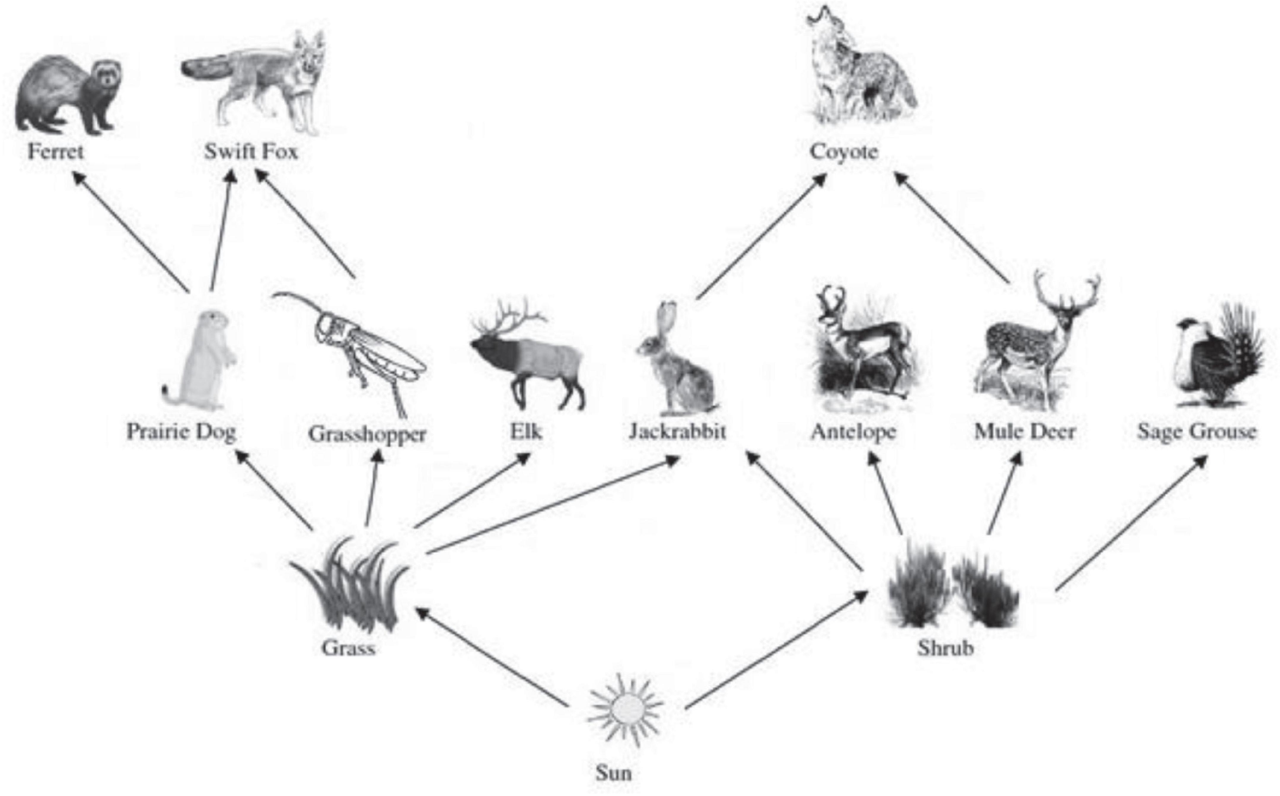
Figure 1. Food web. Food web of 12 native species of a typical sagebrush ecosystem in Southern Wyoming. Grass and shrubs are the two plants. Grass-eating herbivores are elk, prairie dog, and grasshopper. Jackrabbits are both grass- and shrub-eaters. The arrows in the food web show the direction in which biomass and energy flow. The shrub-eating herbivores are antelope, mule deer, and sage grouse. The carnivores are ferret, swift fox, and coyote.

Each species seeks to maximize their net energy. Animal species both expend and generate energy through predation. Some species lose energy through development stress and through energy costs of dispersing in search of higher resource density (Sawyer et al., 2012; Wyckoff et al., 2018). Plant species receive energy from the sun and do not disperse. We parameterize our framework to characterize the food web interactions of the Wyoming sagebrush ecosystem’s 12 species. Key parameters include the average population density per hectare, average annual consumption of biomass for animal species, average annual accumulation for plant species, average life span, gross energy content per kg of biomass, predation risk, nitrogen requirements of plant species, average weight, and basal metabolic rate. We follow previous analyses in defining parameters for our analysis (see data and methods in the Supplement and in Cisneros-Pineda et al., 2020).

The area of study is 109,339 hectares with the Atlantic Rim Natural Gas project creating 15,390 hectares of disturbed areas from its 282 well pads (U.S. Bureau of Land Management, 2007). Two general disturbed areas lie in the area; the main disturbed area occupies 11,173 hectares with 248 well pads and the secondary disturbed area occupies 4,217 hectares with 34 well pads (Figure 2). Three species – sage grouse, mule deer, and elk – experience stress as a function of the intensity of development, the species, and the season (Hebblewhite, 2011; Kauffman et al., 2018). The number of well pads in each disturbed area is a measure of economic intensity to which species respond. We chose a standard of 1 km from development to define a disturbed area in which mule deer, elk, and sage grouse experience stress. Because the stress of development varies across species based on distance sensitivity and other factors, we characterize a ranking of energy-reducing stress in the disturbed areas for these species with mule deer experiencing the most stress, followed by sage grouse and then elk (Powell, 2003; Sawyer et al., 2006; Thomson et al., 2006; Walker et al., 2007; Cisneros-Pineda et al., 2020; Supplementary Material).

FIGURE 2

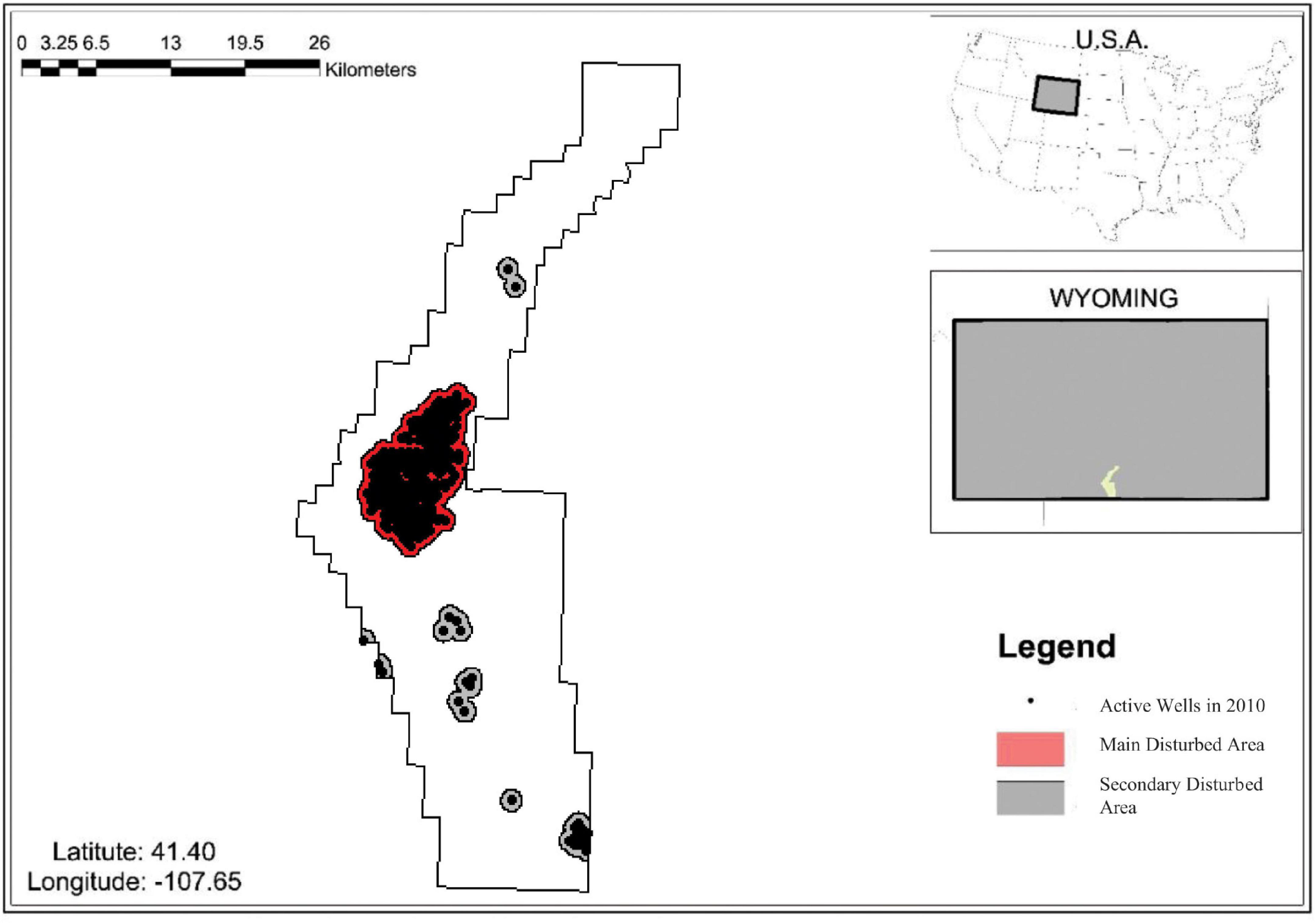
Figure 2. Map of study area: The Atlantic Rim Natural-Gas Development. The black dots indicate the location of active wells in 2010 (U.S. Bureau of Land Management, 2007) and the shaded area indicates the aggregate disturbed areas from a 1 km radius around each well, which is consistent with Powell (2003); Sawyer et al. (2006), and Walker et al. (2007). The upper right two maps show the location of Wyoming and the ARNG inside Wyoming.

Rather than remain in an energy-depleting stressful environment, many species adapt their foraging behavior and location if they can find alternative areas with abundant forage (Van Dyke et al., 2012). To find and move to such areas, each animal incurs a dispersal cost. Each individual balances the energy losses of remaining in a disturbed area with the additional energy sources in other areas, net of the dispersal costs to get to another area. Because they experience higher energy losses from development stress, mule deer and sage grouse disperse and incur dispersal costs at lower levels of development intensity than elk.

To create a tractable stylized landscape for our analysis, we construct a landscape of undisturbed area that surrounds both one main disturbed area and a set of distributed secondary disturbed areas that we treat as one area for management purposes (Figure 3). Species interact within each location and animals can disperse from a disturbed area into the undisturbed area, or the reverse.

FIGURE 3

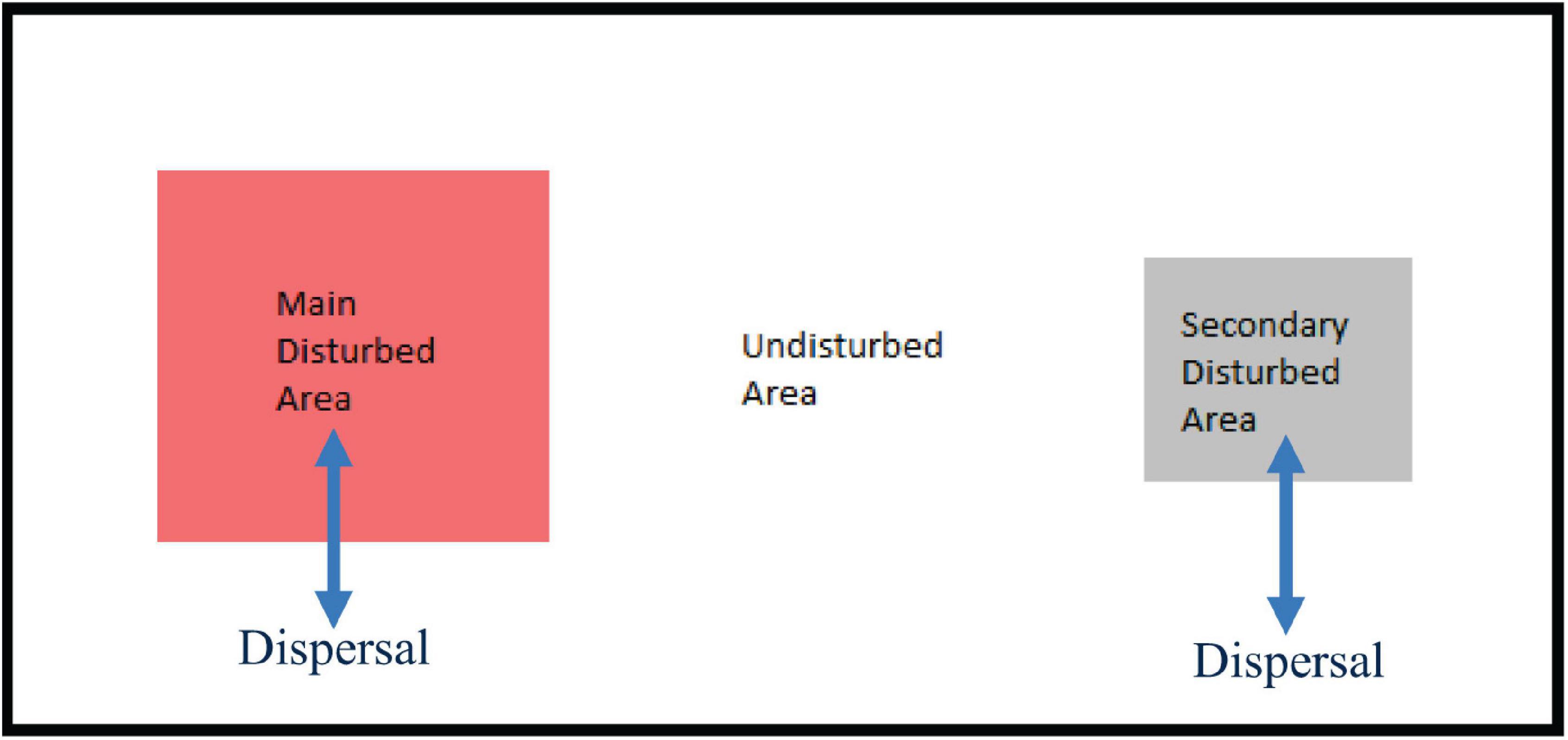
Figure 3. Diagram of undisturbed and disturbed areas. Schematic of the stylized landscape with undisturbed and the main and secondary disturbed areas in which animal dispersal can occur between undisturbed and disturbed areas.

Modeling Framework: Optimization in GEEM

Decisions

A manager seeks to maximize the total population level (n_S(t)) at the time period (t) of the ecosystem steady state $\left(\widehat{t}\right)$ of a target species (S) by allocating a budget $\left(\overline{B}\right)$ to conservation actions in the two disturbed areas. We consider two target species – sage grouse and elk – that are affected by development stress but have different food sources and different dispersal cost levels. How target species and all other species respond to any conservation action is determined through an ecological model of species behavior, interactions, and movement across the landscape. Therefore, the allocation of the budget is a constrained optimization problem subject to the species’ response. We use GEEM as the ecosystem modeling framework that determines the species’ response to conservation actions over which we optimize.

Using GEEM to Capture Species Interactions and Populations Over Time and Space

The GEEM framework conceptualizes species in economic terms to reflect species decisions and interactions based on energy balances (Hannon, 1976, 1979; Finnoff and Tschirhart, 2008). Energy balances in GEEM include gains based on energy embodied in the prey and the losses from the stress associated with disturbances in the ecosystem, from securing prey, and from predation (energy expenditure prices). Energy expenditure prices indicate the scarcity of biomass: when a high number of predators prey upon a relatively low number of prey, energy prices are high.

General Equilibrium Ecosystem Model’s population dynamics involve the transformation of energy into offspring. Biomass consumption and energy expenditure prices are in equilibrium when demand equals supply of biomass. Using these optimal consumption levels of biomass and equilibrium prices, GEEM updates species population depending upon the obtained level of energy. This net energy R_id also accounts for the total cost of dispersal, δ_iβ_iy_id(t), such that the average individual (newcomers and locals) has less energy for reproduction. If individual species are favored by the current conditions of the ecosystem, including disturbances and prey scarcity, and are able to gather extra energy for reproduction, the population increases. The ecosystem is in steady state if all populations remain unchanged in every subsequent period: $t=\widehat{t}$ if n_i(t) = n_i(t + k)∀i species, ∀k subsequent periods.

Animal species move in every period to forage in locations with abundant prey and low competition until the net energy minus the dispersal cost equate in all areas, establishing an arbitrage condition after which no species can change behavior and do better. Depending upon differences in prey scarcity, some animal species adjust the time spent foraging or hunting prey inside the disturbed areas. Individuals allocate more time to seeking prey in areas that offer a higher supply of biomass while considering competitors (inter- and intra-species). As all individuals respond to energy differences, the prey scarcity and the energy expenditure prices increase in those areas. This adjustment mechanism of energy prices leads to an arbitrage condition, where individuals distribute their time preying across the landscape until all areas are equally attractive in terms of net energy gains.

To establish a baseline for conservation actions, we use GEEM to depict the evolution of the landscape from entirely undisturbed to disturbed in two areas, main and secondary. The human development in the ecosystem alters the energetic gains from preying on biomass within the disturbed areas because of the stress that development causes the species. The set of development areas (D), here main and secondary, and the associated stress on all species in each of these areas (ψ) determines the potential energy gains from seeking prey, and GEEM tracks how species behave in response to energy considerations and the prey scarcity.

Constrained Optimization

From that post-development ecosystem equilibrium and steady state as a starting point, the decision maker can partially restore the ecosystem toward its pre-development conditions because the vector of conservation actions (C) reduces development stress, with each component, c_id, of that vector reflecting the level of the action per area, d, for the target species, i. The constrained optimization of the decision maker allocates conservation actions (C) to determine how much conservation action to place in each disturbed areas, subject to a budget constraint and species-ecosystem responses to development:

$$\underset{C}{max}{n}_S\left(\widehat{t}\right)s.t.\{\begin{array}{c}\hfill B(C,D)=\overline{B}\hfill \\ \hfill R_{id}^{*}=\underset{X_{id}\left(t\right)}{max}{R}_{id}(E_{id}\left(t\right),X_{id}\left(t\right))-\left(1-c_{id}\right){\mathrm{\psi }}_{id}\hfill \\ \hfill \frac{n_{id}\left(t+1\right)-n_{id}\left(t\right)}{n_{id}\left(t\right)}={\mathrm{\sigma }}_i(R_{id}^{*}-\frac{{\mathrm{\delta }}_d{\mathrm{\beta }}_i{y}_{id}\left(t\right)}{n_{id}\left(t\right)},X_{id}^{*},E_{id}^{*})\hfill \\ \hfill \frac{R_{i{d}_1}^{*}-R_{i{d}_2}^{*}}{{\mathrm{\beta }}_i}\le {\mathrm{\delta }}_d\mathit{\hspace{1em}\hspace{1em} }\begin{array}{c}\hfill \forall ispecies\hfill \\ \hfill \forall dareas\hfill \end{array}\hfill \end{array}(1)$$

where i, d, and t indicate the species, the area in which the species is located, and the time period, respectively; ψ_id is the stress experienced by the i-th species; E_id(t) represents the energy expenditure “prices” related to the species (prices paid by its predators and by animal species to consume prey or by plant species to accumulate photosynthetic biomass); X_id(t) represents the biomass accumulations (plants) or consumption (animals) of all prey of the species; B(…) is spending as a function of costs for the conservation actions with a maximum budget of $\overline{B}$; R_id(…) is the function that defines the net energy accumulated during the current time period and $R_{id}^{{}^{*}}$, $X_{id}^{{}^{*}}$, and $E_{id}^{{}^{*}}$ are the optimum net energy, biomass, and energy expenditure prices, respectively, of the current time period; y_id(t) is the number of individuals that dispersed into the area during the current period; n_id(t) is the population of species i in area d (that already considers the dispersed individuals); δ_d is the dispersal cost to move across areas and it is a proportion of the metabolic rate of the species, β_i; and σ_i(…) is the net growth rate of species i.

Dispersal

Both development and conservation actions alter how animals move and forage because these interventions alter the ratio of prey to predator and can make some locations difficult to access. The species dispersal rule is given by the differential of net energies between two areas: $R_{i{d}_1}^{{}^{*}}-R_{i{d}_2}^{{}^{*}}$. Because the net energies that drive the dispersal decision are based upon a maximization of net energy of all individuals in the ecosystem, the dispersal rule accounts for animals that indirectly change energy prices due to increasing the number of predators of the species’ prey and by increasing the number of prey for its own predators. If the potential gain of net energy between two areas is not large enough to compensate for the dispersal cost, then no movement occurs.

Disturbances and Conservation Actions

The model in eq. (1) introduces the parameter ψ_id to represent the energetic cost (measured in kcal) associated to the stress of enduring human disturbances, such as energy development. Not all species (in the application of this paper: plants, some small mammals, and carnivores) experience stress and species that are sensitive to the disturbance (elk, mule deer, and sage grouse) only experience stress when they are located inside the disturbed areas. The energetic losses from this stress are associated with different types of factors such as traffic, human presence, or noise that affect different species differently (Blickley et al., 2012). By assumption, ψ_id =  0 before any economic activity or human disturbance is introduced into the ecosystem. Once disturbances are introduced to the ecosystem, the net energy that affected species gather inside the disturbed areas is reduced by a fixed amount, which generates incentives to disperse into the undisturbed area: R_{i,Undisturbed} > R_i,Disturbed before dispersal. The stress experienced by the target species i in the main and secondary disturbed areas can be reduced by conservation actions in the respective area: (1−c_id)ψ_id. The decision maker can reduce some of the damages that cause energetic losses from stress by choosing a level of investment of conservation actions c_id. These conservation actions include reduction of economic activity, such as limiting traffic, noise, and lights or improvement of habitat constraints, such as providing water sources.

Conservation Costs

For conservation actions that reduce stress, the cost of conservation actions depends on the economic intensity of the disturbed area and the level of uniform conservation effort employed in each disturbed area:

$$B(C,D)=\sum _{d\in D}{A}_d\frac{c_{id}}{1-c_{id}}(2)$$

where A_d is the economic intensity of the different disturbed areas, c_id is the conservation effort employed in area d for target species i, and $\frac{c_{id}}{1-c_{id}}$ measures the cost per squared unit of conserved area. In this specification of the model, the marginal cost of conservation increases as stress nears eradication; costs become infinite at low stress levels, making complete restoration of the ecosystem impossible, $\underset{c_{id}\to 1^{-}}{lim}\frac{c_{id}}{1-c_{id}}=\mathrm{\infty }$. This functional form represents the case where investing in a single location has increasing marginal costs, but it also shows that larger disturbed areas are harder to intervene.

For conservation actions that reduce dispersal costs in our second analysis, we alter the conservation effort c_d in equation (1) to reduce the dispersal cost in all d disturbed areas for all species, instead of reducing the stress ψ_id for one target species. In this case, the allocation of conservation budget across the disturbed areas addresses barriers that prevent movement of animals in/out of those locations. Dispersal between the undisturbed area and the disturbed area d when conservation actions reduce the dispersal cost becomes:

$${\mathrm{\delta }}_d=(1-c_d){\mathrm{\delta }}_0(3)$$

where δ₀ is the initial dispersal cost common to all species and δ_d is the dispersal cost following conservation actions to reduce that cost in area d.

Naïve Model

Although the constrained optimization decisions follow the same steps for the naive and complex food webs, in the naïve model, the system of equations in (1) is simpler because it contains only 2 species (i=2): the equations that relate to one plant prey species and the target species for the disturbed and undisturbed areas. Because other animal and plant species are absent in the naïve model, the plants’ losses from grazing and competition for sunlight are understated in the naïve model. The population of herbivores is not regulated by the potential predation from carnivores. In the complex model, all plant individuals react to the additional grazing pressure whenever animal species disperse into an area (disturbed or undisturbed), but the plants of one species also react to the other plant species’ reactions to dispersal. Other plants are relevant because they may face higher (lower) relative pressure, shrink (expand), and open (reduce) space for competitor plants. In contrast, in the naïve model, the plants (grass or shrubs) only react to the additional grazing pressure from one target species (elk or sage grouse). Similarly, in the complex model, the scarcity level of plants during each period is a consequence of the aggregated grazing pressure of local and newcomer foragers and the reactions of foragers to their predators. The naïve model lacks the interaction of dispersal from multiple animal species and scarcity of biomass from multiple plant species. For example, when elk in the naïve model disperse into the undisturbed area from disturbed areas, grass in the undisturbed area faces higher grazing pressure but the reaction of shrubs to sage grouse and mule deer dispersal is ignored.

Analysis

We conduct two types of analysis to address two different conservation questions.

How Do Conservation Actions Differ Between Naïve and Complex Ecosystem Models?

To evaluate the common simplifying assumption of a naïve species model to inform conservation decisions, we calculate and compare the optimal conservation budget allocation for both the 2-species naïve model and the 12-species complex model and the population distributions that result following those actions and species response. We examine two naïve models - sage grouse and shrub; and elk and grass. The target species experiences stress whenever it forages close to the development area, while its food is a plant species that experiences no development stress. For the complex setting of 12 species, of which three species experience development stress, we solve the optimization for both sage grouse and elk as the target species. As a starting point for analysis, we use the steady state that arises after development and impose conservation actions on that steady state, which produces another transition of ecosystem response to a post-conservation steady state. Because the solution to equation 1 is not closed, we run the naive and complex GEEM models until a steady state is reached using Mathematica 12.1.

How Do Dispersal Costs Influence Populations Across the Landscape and What Allocation of Conservation to Reduce Dispersal Costs Most Benefits Populations?

In this set of analyses, we begin with the undisturbed steady state and define the steady state that evolves after the disturbance in the two disturbed areas for a range of dispersal costs. Next, we evaluate the impact of conservation actions that reduce dispersal costs from the point of the initial disturbance, meaning that the system is not in steady state following the development disturbance but instead moves toward the new steady state while experiencing the conservation actions that encourage dispersal by lowering costs.

Results and Discussion

In the first section here and to establish a point of comparison, we present and discuss how the undisturbed system responds to disturbance, as from development, in two locations in the landscape. We identify the long run steady state populations of the naïve model focused on sage grouse, naïve model focused on elk, and the complex ecosystem model in each of the disturbed areas and the undisturbed area. In the next section of analysis, we use those post-disturbance steady states as the initial landscape and determine the optimal allocation of conservation spending across the 2 disturbed areas to improve target species populations. We compare the conservation decisions and the species outcomes across the naïve and complex models to inform a discussion about the policy-relevant species responses that naïve food web models ignore. In the following section of analysis, we identify and describe how species’ dispersal costs lead to different distributions of species in response to the initial disturbances. Through the lens of species interactions, we then describe the impact of policies to reduce dispersal costs during disturbance to enable species to more readily move away from the disrupted habitat.

Baseline

Baseline Results

The initial undisturbed landscape comprises populations of 12 species in the complex model and the target and its prey for the naive models, distributed across the pre-defined areas that will be disturbed and undisturbed (Table 1). This population distribution is the long run steady state outcome of species growth and movement across the landscape. Using that initial landscape condition, the system responds to disturbance in a main and secondary disturbed area through dynamic interactions of species including dispersal of species, arriving at a long run steady state of populations after adjusting to the disturbance (Table 1, “post-disturbance” row for every relevant species). In the naïve model that considers only sage grouse and their food source (shrubs), the disturbed areas lead to an increase in sage grouse population in the disturbed areas and no change in the undisturbed area, resulting in an overall increase of the population (Table 1, row 8). In the naïve model that considers only elk and their food source (grass), elk populations decline in both disturbed areas and remain unchanged in the undisturbed area, leading to a decrease on the landscape in total in response to the disturbance (Table 1, row 4). In contrast, in the complex model, the population of sage grouse decreases in all areas for a total decrease on the landscape while the population of elk decreases in the disturbed areas and increases in the undisturbed area for a total decrease on the landscape (Table 1, rows 12 and 16).

TABLE 1

Table 1. Impact of disturbances on the species populations.

Explanation

The naïve models’ lack of species competition drives the differences in system response to disturbance between naïve and complex models. Following the disturbance, because there is no competition with other shrub-eaters nor predators in the naïve model, the sage grouse disperse from both disturbed areas into the undisturbed area until they experience no further gains in net energy from dispersing. In the long run, however, less predation in the disturbed areas and no competition for sun in this naïve model allow shrub biomass to grow, which compensates for the disturbance for sage grouse. The naïve model’s lack of species competition leads to a prediction that the sage grouse is better off in the long run following development creating disturbed areas. Similarly, elk experience stress inside the disturbed areas and respond by dispersing to undisturbed areas. The movement of elk reduces grazing pressure on grasses inside the disturbed areas, and the supply of biomass increases, but not enough to offset stress on the remaining elk in the disturbed areas. In contrast, the complex food web includes the response of other shrub-eaters and grass-eaters to the reduced grazing pressure of sage grouse and elk in the disturbed areas. Facing that competition for food sources, both sage grouse and elk remaining in the disturbed areas decline in population. Similarly, sage grouse and elk that disperse to the undeveloped areas face competition for scarce resources there, with resulting declines in population for sage grouse and a mild increase for elk. The population of elk in the undisturbed area grows in the long run due to an increased abundance of grass, which out-compete the overgrazed shrubs. In both cases, because the naïve food web models do not consider species interactions, they lead to different predictions for the disturbances long run impact on population sizes across the landscape.

Interpretation and Meaning

These results demonstrate the role of species interactions within a food web for determining the system’s response to heterogenous disturbance in the landscape. We use the post-disturbance steady state populations as an initial landscape condition in the following analysis of conservation actions post-development and as a point of comparison in the subsequent analysis of dispersal costs and actions to reduce dispersal costs.

Conservation Actions Across Naïve and Complex Species Interaction Models

Using the 3 steady state population distributions for the naïve-sage grouse, naïve-elk, and complex models as an initial landscape condition, we determine the optimal portion of a conservation budget to place in the main and secondary disturbed areas considering and contrasting the goal of maximizing sage grouse populations versus elk populations on the landscape.

Sage Grouse as the Target Species for Conservation Action

Results

To maximize sage grouse population on the landscape in the naïve model, the optimal allocation of the conservation budget is to do no conservation in either disturbed area (Table 2, row 2). Any conservation actions to reduce stress on sage grouse on the landscape lead to fewer sage grouse. In contrast, in the complex model case, sage grouse populations are maximized by allocating most of the budget to the secondary conservation area (82%) (Table 2, row 4). In the complex model, this conservation action increases the population of sage grouse in both disturbed areas, maintains the population in the undisturbed area, and increases the population overall (Table 2, row 4). The optimal conservation actions produce these population responses to reverse 20.3% of the development’s impact on sage grouse (Table 2, column 6).

TABLE 2

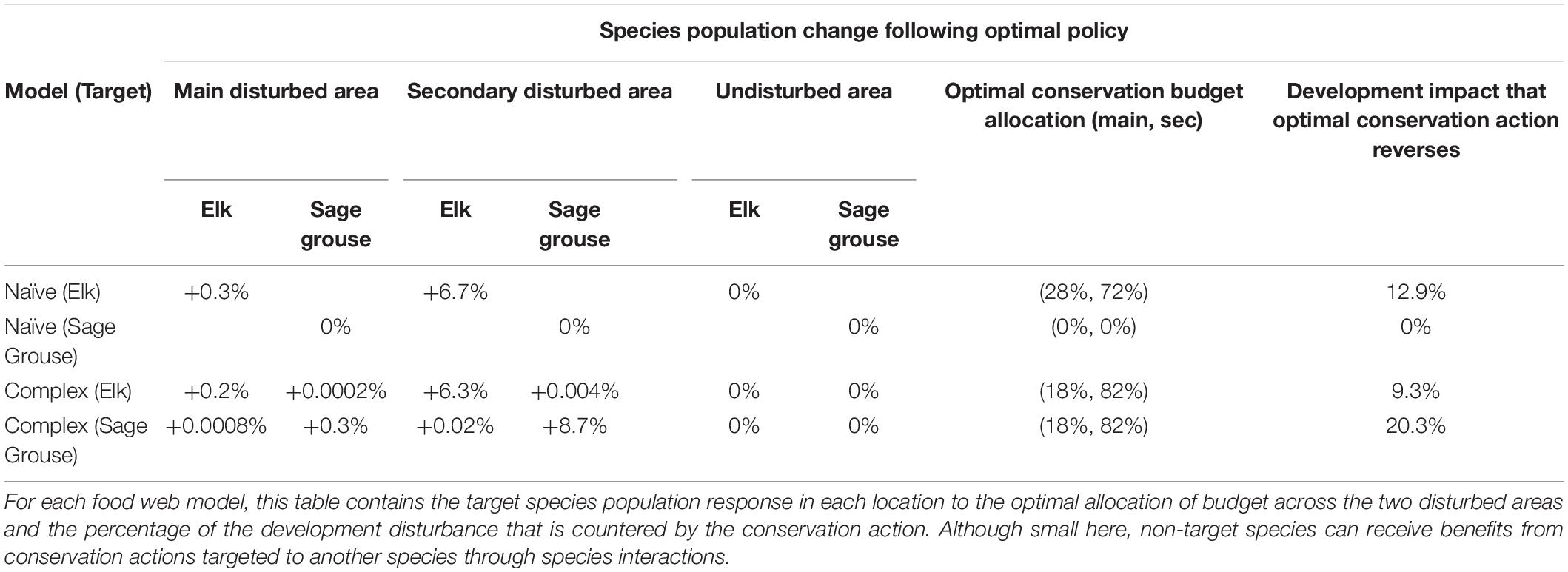
Table 2. Impact on the species populations of conservation actions that reduce stress.

Explanation

In the naïve model, any conservation action causes sage grouse to overcrowd the now-improved disturbed areas in search of less scarce food. The new sage grouse offspring that result from lower stress in the disturbed areas quickly increase the scarcity of shrub forage, which more than compensates for the conservation action’s reduced stress. In this case, sage grouse grazing overwhelms the shrubs’ growth and sage grouse do not benefit from the conservation actions. In the complex model, conservation actions do not induce such overcrowding and the conservation actions have a positive impact on the population. If the naïve (2-species) model’s optimal conservation action – here, no conservation action – is applied to the complex (12-species) setting, no conservation gains accrue. That finding implies that using the naïve model to determine policy misses the opportunity to capture the 20.3% reduction in development impact that the conservation plan from the complex model achieves (Table 2, row 4). Ignoring the species interactions by basing decisions on the naive model leads to too little conservation action to mitigate development impact.

Interpretation and meaning

The naïve model over-emphasizes the role of crowding disturbed areas due to that framework’s lack of other species interactions, leading to missed opportunities for conservation.

Elk as the Target Species

Results

Unlike the sage grouse naïve model, the optimal conservation based on both the naïve and complex models allocate conservation actions to both disturbed areas (Table 2, row 1). The naïve model’s optimal allocation of conservation funding puts the majority of the budget, 72%, into conservation actions in the secondary disturbed area (Table 2, row 1). Similarly, the complex model finds an optimal allocation that even further emphasizes the secondary area (82%), which counters 9.2% of development’s impact on elk (Table 2, row 3). The emphasis on the secondary disturbed area comes from its relatively small size, which allows conservation actions to have a larger impact per unit of spending there. Both the naïve and complex models’ optimal conservation actions lead to increases of the elk population in both disturbed areas, no long run impact on elk population in the undisturbed area, and increases in the elk population overall.

Explanation

In the naïve model, the conservation actions do not cause elk to overcrowd the disturbed areas because the available grass can sustain a larger population of elk. In both models, the optimal conservation action lowers stress in the disturbed areas, which increases the net energy elk accumulate and translates into a higher population. Elk do not disperse from the undisturbed area to the now-improved disturbed areas because the potential gains are not large enough to compensate for the dispersal cost. In both naïve and complex models, the conservation actions allow the total elk population to grow due to reduced stress in both disturbed areas. The complex model’s optimal conservation reduces the population cost of disturbance by 9.2% but using the naïve model’s conservation allocation in the presence of multiple species interactions reduces that population cost by only 8.9%. Therefore, using the naïve model to define policy misallocates conservation funding and misses 3% of potential conservation gains.

Interpretation and meaning

The naïve and complex model lead to different conservation budget allocations. If the complex system holds but the naïve model’s allocation of conservation spending occurs, the planner overspends in the main disturbed area and generates fewer conservation benefits. The central difference between the naïve and complex models’ conservation response comes from the complex model’s inclusion of grazing pressure from grass-eaters other than elk.

Conservation Action Impact on Non-target Species

Conservation actions on a target species may indirectly benefit other species that also experience development stress and that interact with the target species through the food web (Table 2). For example, conservation actions in a disturbed area directed at elk raise grazing pressure on grass, which lowers the density of the preyed plant (grass) and opens space for competitor plants (shrubs). Other species that prey on the competitor plant (shrubs) indirectly benefit from increased abundance of their prey plant, despite the conservation actions being aimed at other species. In contrast, species that compete over the same plant species with the target species can find that increased competition due to the increase in competitor species leaves them worse off following the conservation. For example, when elk is the target species, conservation actions make mule deer and sage grouse better off (see Table 2, rows 3 and 4). In the complex food web case, the impact of conservation actions targeted at sage grouse have little impact on the populations of the other stressed species in the disturbed areas (elk and mule deer) because biomass consumption of sage grouse is small relative to the consumption of ungulates. The optimization of conservation actions using a simple food web ignores key mechanisms behind the predator-prey relationships. Because oversimplified species models ignore species interactions, they cannot be used to identify the positive or negative impact of conservation actions on non-target species.

Discussion

Differences across the food web models arise because the more complex model assess inter- and intra-species competition over resources. Development disturbances that affect sage grouse lead to declines in that species population in the complex model but the naïve model predicts that sage grouse populations increase following development because it ignores species competition for forage. Optimal conservation actions to mitigate the development disturbance also differ across the two models, which generates lower conservation outcomes when applying the naïve model’s policies to a system that contains more species as in the complex food web. In contrast, the models predict similar populations and similar conservation actions when elk are the target species, although again the naïve model’s policy wastes conservation spending if applied in a setting with broader species interactions. Although simple predator-prey models are common in economics and in management, their inability to reflect disturbance- and conservation-induced changes in the broader food web and species interactions limits their usefulness in describing disturbance impact on metacommunities and in establishing efficient conservation policy.

The Impact of Costly Dispersal on Conservation Actions and Outcomes

Species adjust to development activities that generate heterogeneity across the landscape – here, a main and secondary disturbed area and an undisturbed area – by altering their behavior, experiencing stress, and dispersing to other locations to access resources. Because dispersal decisions reflect energy balances, the long run species population response reflects the size of the energy costs that dispersal imposes. Species disperse as a function of their stress levels, metabolic rate, and cost of dispersal, all of which vary across species. Here, three species – elk, sage grouse, and mule deer – experience stress from development and have incentives to disperse from disturbed areas. Coyotes do not experience stress but will disperse given low enough dispersal costs and in reaction to their dispersing prey, mule deer. Other food web species are connected to the stressed species through plants but are not directly affected by disturbance.

To establish a baseline and to understand the impact of dispersal costs on metacommunities, we show how different initial dispersal costs alter the distribution of species across the landscape when a disturbance is introduced into the ecosystem. Next, we explore the impact of conservation actions that reduce the cost of dispersal for all species, revealing circumstances in which the reduction of dispersal costs leads to undesired results for the target species due to species interactions. Last, we describe the case where the conservation actions cannot target a specific species and instead reduce dispersal costs for all species.

Impact of Dispersal Costs on Metacommunities

Results

The naïve food web models predict no difference in species population distribution across dispersal costs. In the complex model, the impact of the level of dispersal costs on population distributions varies across species. Due to their stress response to development, sage grouse, mule deer, and elk disperse across the landscape at higher rates than other species at all dispersal costs. A very high dispersal cost (1.25) implies that no species disperse given a moderate level of development stress; a very low dispersal cost (0.01) denotes an ecosystem where coyotes disperse; and an even lower dispersal cost allows small species, such as jackrabbits and prairie dogs, to disperse. All 3 stressed species disperse for dispersal costs below 0.75; mule deer and sage grouse also disperse for dispersal costs between 0.75 and 1.0; and mule deer disperse for dispersal costs between 1.0 and 1.25. Across all levels of dispersal costs, at higher dispersal costs, sage grouse populations are lower in disturbed areas but larger in the undisturbed area and in total on the landscape (Figure 4). In contrast, at higher dispersal costs, elk populations are higher in disturbed areas and lower in undisturbed and in total on the landscape (Figure 4).

FIGURE 4

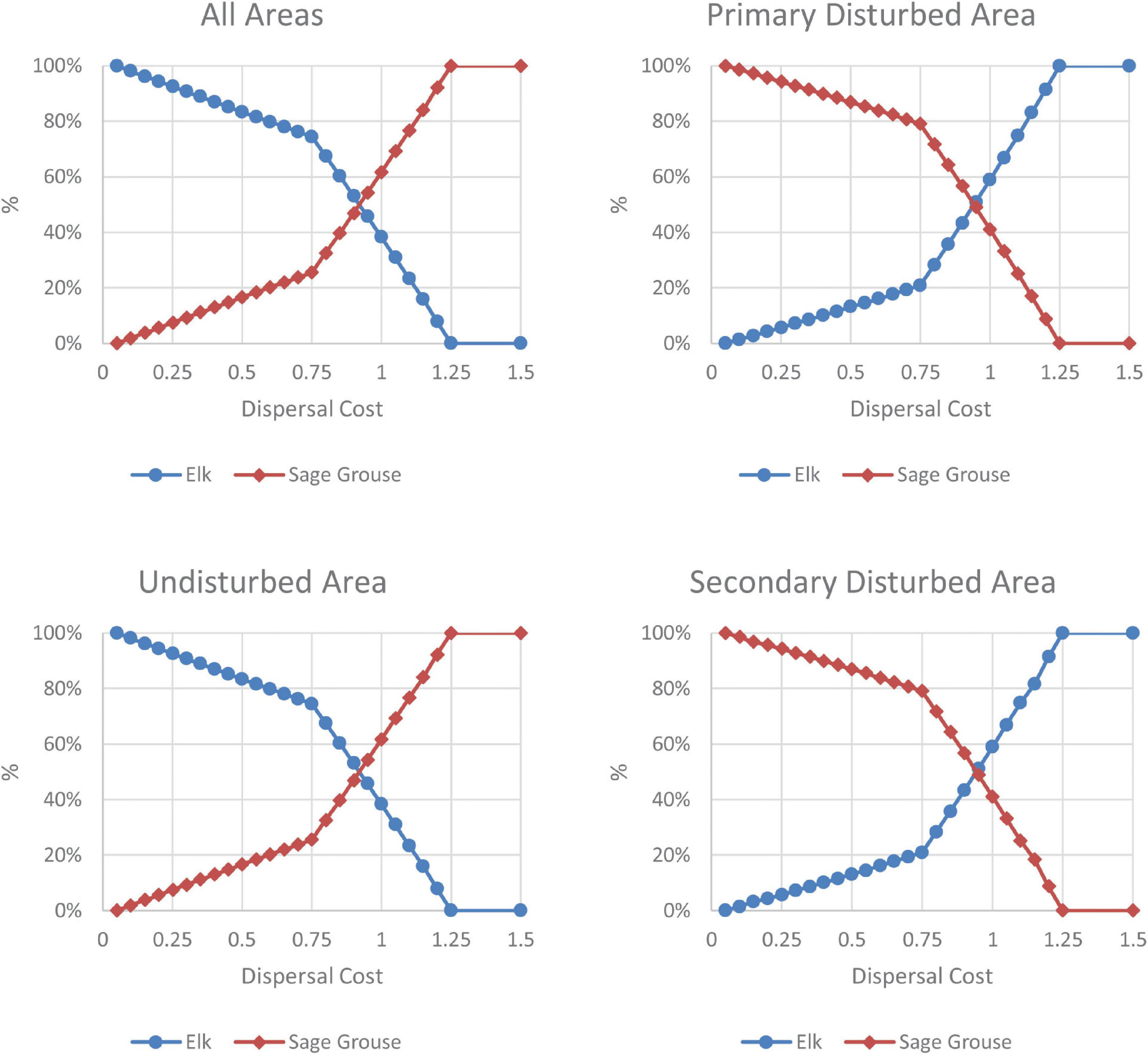
Figure 4. Population distribution after development across dispersal costs. For the landscape and each sub-area, the graphs depict the percentage of the maximum population for elk and sage grouse at the post-disturbance steady state across dispersal costs in the complex model. The graphs are normalized such that 100% is the highest possible population and 0% is the lowest possible population at the post-development steady state in each area for that species. This normalization relates to the highest and lowest possible populations in each location; it does not imply that a species population goes to zero in an area nor does it imply that species population is not hurt by development.

Explanation

In the complex food web model, dispersal costs combine with species interactions between dispersing and non-dispersing species to determine the populations across the landscape following development. At dispersal costs below the level that prevents dispersal (1.25), the development-stressed species that disperse from the disturbed areas to the undisturbed areas change the species competition and resulting populations in all areas. At low dispersal costs when all development-stressed species disperse (below 0.75), the mule deer and sage grouse’s impact on shrubs dominates outcomes: enough shrub-eaters disperse from the disturbed areas to the undisturbed area that they overgraze shrubs in the undisturbed area, allowing grass and grass-eaters like elk to thrive in the undisturbed areas. Sage grouse that remain in the disturbed areas gain from the reduced competition for shrubs there. At high dispersal costs with no elk dispersing (above 0.75), resident elk in the undisturbed area no longer face competition with dispersing elk. Although sage grouse and mule deer disperse, higher dispersal costs mean fewer individuals disperse, which limits the intra-species competition in the undisturbed areas and sage grouse do well there. At high enough dispersal costs (at and above 1.25), no species disperse, which means that species in the undisturbed area face no new inter- or intra-species competition and the impact of development accrues only to the individuals in the disturbed areas.

Interpretation and meaning

The dispersal cost determines which type of species (grass- vs. shrub- eater) is most negatively affected by development after species disperse and interact in each portion of the landscape. Here, total landscape elk populations are more profoundly affected by development when dispersal costs are high and total landscape sage grouse populations are most affected when dispersal costs are low due to the levels of dispersal of all species and the resulting competition for food. In contrast, individual elk in the disturbed area are least negatively affected by development when dispersal costs are high, while the opposite holds for sage grouse in the disturbed areas. The complex food web model and the naïve model predict different responses to dispersal costs because the naïve model does not consider the species interactions that differ across dispersal cost levels.

Impact of Conservation Actions to Reduce Dispersal Costs

Because dispersal costs stem from energy losses due to searching for new resources or expending energy to surmount barriers, some types of conservation actions like watering holes and wildlife bridges can reduce the dispersal costs that all species face. In contrast to the above conservation actions that occur long after disturbance, here, the dispersal cost-reducing conservation actions occur at the time of disturbance.

Results

Policies to reduce dispersal costs have no impact in either of the target species cases for the naïve food web model because those models contain no species interactions that drive the impact of dispersal costs. In the complex model, sage grouse do not benefit from any reductions in dispersal costs from initial levels of such costs above negligible levels.

In the complex model, elk populations gain from conservation actions that decrease dispersal costs for all species, with three ranges of emphasis across disturbed areas (Figure 5). For the target species elk in the complex model, reducing dispersal costs from initial dispersal cost levels below 0.75 (0.01–0.55, range 1, Figure 5) leads to increases in the elk population from an optimal distribution of conservation efforts across the disturbed areas that emphasizes conservation in the secondary disturbed area. At initial dispersal costs in the next highest range (0.55–0.82, range 2, Figure 5), conservation actions to reduce dispersal costs have a high marginal impact on elk populations from a distribution of conservation actions that focuses on the main disturbed area. Reducing dispersal costs from that range of initial dispersal costs encourages dispersal of sage grouse and mule deer without dispersal from elk, which leads to overgrazing of shrubs in the undisturbed areas and benefits to resident elk there. At still higher dispersal costs (0.82–1.25 and above, range 3 Figure 5), elk populations respond positively to conservation actions to reduce dispersal costs that are increasingly balanced across the disturbed areas but do not reduce costs enough to induce elk to disperse. At the highest level of initial dispersal costs (1.25), the optimal allocation of conservation is 59% in the secondary disturbed area and 41% in the primary disturbed area. At very low dispersal costs (below range 1), the optimal conservation policy for target species elk is to not allocate any resources to reduce dispersal costs in either disturbed area.

FIGURE 5

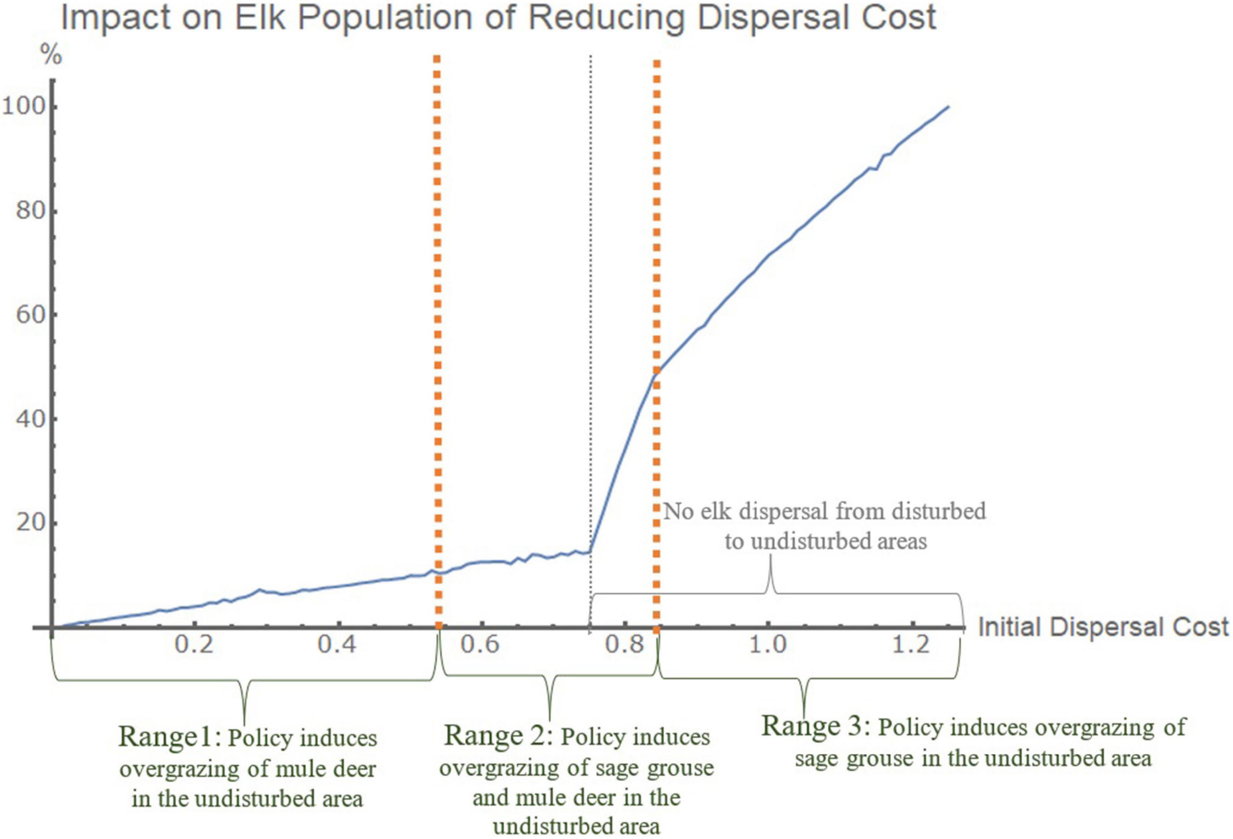
Figure 5. Conservation actions that reduce the dispersal cost of all species (Complex Model, target Elk). The graph shows the impact of optimal conservation budget allocations on elk populations (vertical axis) for the complex model across different initial dispersal costs (horizontal axis). The graphs are normalized such that 100% is the highest possible impact and 0% is the lowest possible impact for this dispersal cost conservation policy. The x-axis is the initial dispersal cost but the response of the elk population is to the optimal policy reduction in those dispersal costs from that initial dispersal cost.

Explanation

Because species respond to stress and dispersal costs differently, the outcomes from conservation actions at the time of disturbance that reduce dispersal costs depend on the initial dispersal costs. For example, for dispersal costs above 0.75, actions to reduce dispersal costs promote the dispersal of sage grouse and mule deer but dispersal costs still prevent dispersal of elk. In that range, the dispersal of sage grouse and mule deer to the undisturbed areas increases pressure on shrubs, which increases grass and elk populations in the undisturbed areas, while elk remaining in the disturbed areas are slightly worse off. Even though no elk disperse, the overall population of elk is better off due to the other species’ dispersal and the resulting species interactions that produce energy gains for elk in the undisturbed area. Because elk do not disperse, they do not cause overgrazing of grasses in the undisturbed area that would lead to declines in the total elk population. At lower initial dispersal costs (below 0.75), however, more species and individuals disperse without conservation interventions, including elk as the target species. In these cases, conservation actions in the secondary disturbed area provide total elk population increases, even though elk in the main disturbed area may not disperse away from that disturbance. Reducing dispersal cost to very low levels (below range 1) leads to a decline in overall elk population because the damages from increased foraging move beyond the disturbed area to other areas.

Interpretation and meaning

Due to species interactions, total landscape populations of elk are higher when elk do not disperse from disturbed areas to impose costs on elk in undisturbed areas. If they disperse, the dispersal makes non-dispersing individuals better off in the disturbed areas but the dispersers make the individuals in undisturbed areas worse off. Optimal budget allocations for conservation contain the overgrazing of elk by preventing their dispersal while encouraging other species to disperse. The dispersal of those species alters species competitions in disturbed and undisturbed areas that favor elk populations overall. Because the landscape is in energy equilibrium prior to the disturbance², dispersal from the disturbed area has a negative impact on the undisturbed area; the impact of the disturbance spreads from the disturbed area through species dispersal and species competition in the undisturbed area. Dispersal costs that are too low cause a negative externality from development in the disturbed area to the undisturbed areas that operates through elk dispersal at low dispersal costs.

Discussion of Dispersal Costs

In general, the lack of inter-species competition causes dispersal costs to have no impact on the predictions of the naïve model. Policies to mitigate the impact of disturbance by encouraging the movement of species away from disturbed areas by lowering dispersal costs cannot rely on naïve models of food webs.

Many bio-economic frameworks consider species dispersal without capturing species decisions about dispersal, including those based on dispersal costs. Because some species respond to disturbance and dispersal costs differently from others, the types of species interactions that occur on the landscape differ across dispersal cost levels. Standard models that ignore such dispersal costs lead to more homogeneous distributions of species and to different metacommunities than those that reflect such costs. As above, we also find important differences between the species populations and distributions between the naive and complex model because the naïve models’ species populations and distributions do not vary across dispersal costs. In the complex models, actions that reduce dispersal costs for all species can improve populations in some cases. No dispersal cost reductions improve sage grouse populations but particular ranges of those reductions can help elk populations. In a counter-intuitive result, higher elk populations occur when reductions in dispersal costs lead to dispersal of other species while elk remain in the disturbed areas. Managers can consider thresholds that induce dispersal across species and investigate the system response to the species interactions following dispersal to determine where and how much to reduce dispersal costs to induce species dispersal and interactions that benefit their target species.

High enough dispersal costs keep species from adjusting to disturbance by dispersing. That lack of dispersal means that the negative impact of the disturbance is contained in the disturbed area. Dispersal itself can act as a mechanism to extend the impact of disturbance to other areas of the landscape, here by intensifying grazing in undisturbed areas. Frameworks that ignore dispersal costs likely overstate the impact of this negative externality while frameworks that assume species do not spread from disturbed areas understate that impact.

Conclusion

This analysis explores the impact of two common simplifications used in spatial bioeconomic analysis to determine conservation policy: simple food webs and zero species dispersal costs. In both cases, we find that decisions made with these simplifications lead to policy that misses conservation opportunities. Species interactions within disturbed and undisturbed portions of a heterogeneous landscape following dispersal drive the distributions and levels of species populations and can be leveraged to generate conservation.

First, comparing the metacommunities from a naïve 2-species food web model to those from a more complex 12 species food web model, we find that analysis based on naïve and complex food web models lead to different conservation policies. Applying policy derived from the naïve model to a landscape with complex metacommunities misses opportunities to achieve higher target species population levels. In this framework, because the naïve model ignores the indirect impact of overgrazing from other species and individuals, using it to define optimal conservation leads to wasteful allocation of conservation budget across disturbed areas. Using food web models that reflect species interactions improves conservation outcomes because they predict the responses of all species, including dispersal and forage competition, that determine the outcome for the target species and all metacommunities on the landscape.

Second, novel conservation actions include those that ease dispersal of species across a landscape, such as wildlife bridges, but choosing such actions requires analysis of the response of metacommunities to dispersal costs. We define the impact on species populations and distributions across a heterogenous landscape in response to different dispersal costs, which identifies that the naïve food web model’s populations do not vary across dispersal costs. Because species vary in their response to disturbance and to dispersal costs, managers can use conservation actions that reduce dispersal costs enough to cause some species to disperse but not enough to induce much dispersal from other species in order to leverage species interactions; here, dispersal cost reductions that induce sage grouse and mule deer to leave disturbed areas while elk do not disperse leads to species interactions in all areas of the landscape that increase total elk populations. In addition, dispersal of species from a disturbed area to undisturbed areas widens the area of impact of the initial disturbance; species dispersal acts as a mechanism to create a spatial externality from the original disturbance. Basing policy on frameworks that ignore dispersal costs misses opportunities to improve conservation outcomes and ignores relevant spatial ecosystem externalities.

These analyses raise concern about overly simple frameworks for making conservation decisions for heterogenous landscapes of metacommunities of species that interact within locations and across locations through dispersal. Still, our complex system has only 12 species, which raises questions about the appropriate degree of simplification of these systems. In one consideration, the framework used here, GEEM, is simple enough to be tractable for policy analysis. In another consideration, the results here depict the importance of incorporating enough species to reflect competition for space by the prey species – here, grass and shrubs – to discern how predator populations – here, elk and sage grouse – interact through that prey competition. For example, in this system, the impact of elk overgrazing in an area leads to shifts in the prey species that support the other predator species, sage grouse. While no one level of complexity will prove appropriate in all policy settings, these analyses suggest that identifying and including the primary species interactions in a location and across locations improves conservation policy.

Data Availability Statement

The original contributions presented in the study are included in the article/Supplementary Material, further inquiries can be directed to the corresponding author/s.

Author Contributions

HA and AC-P conceptualized the analysis, evaluated the results, developed insights, and shared writing responsibilities. JT built GEEM and contributed insight. AC-P augmented the simulation code in Mathematica and performed all computational work. HA identified questions. All authors contributed to the article and approved the submitted version.

Conflict of Interest

The authors declare that the research was conducted in the absence of any commercial or financial relationships that could be construed as a potential conflict of interest.

Publisher’s Note

All claims expressed in this article are solely those of the authors and do not necessarily represent those of their affiliated organizations, or those of the publisher, the editors and the reviewers. Any product that may be evaluated in this article, or claim that may be made by its manufacturer, is not guaranteed or endorsed by the publisher.

Acknowledgments

We dedicate this work to our co-author JT.

Supplementary Material

The Supplementary Material for this article can be found online at: https://www.frontiersin.org/articles/10.3389/fevo.2021.707375/full#supplementary-material

Footnotes

1. ^ Grass is comprised of Idaho fescue (Festuca idahoensis), prairie junegrass (Koeleria macrantha), bluebunch wheatgrass (Pseudoroegneria spicata), Thurber’s needlegrass (Achnatherum thurberianum), needle and thread (Hesperostipa comata), squirreltail (Elymus elymoides), and Sandberg bluegrass (Poa secunda). Shrubs are comprised of Artemisia tridentata Nutt. from the Wyoming big sagebrush and the mountain big sagebrush ecosystems (Davies et al., 2010, p. 462–464).
2. ^ An underlying assumption of GEEM is that the undisturbed ecosystems have allocated resources and species in the most efficient way through mechanisms of species evolution, which means that species cannot move to improve the population outcomes in undisturbed areas.

References

Albers, H. J., Kroetz, K., Sims, C., Finnoff, D., Horan, R., Rongsong, L., et al. (2021). Integrating economics and ecology for seasonal migratory species conservation. Rev. Environ. Econ. Policy (in review).

Google Scholar

Albers, H. J., Preonas, L., Capitan, T., Robinson, E. J. Z., and Madrigal, R. (2020). Optimal siting, sizing, and enforcement of marine protected areas. Environ. Resour. Econ. 77, 229–269. doi: 10.1007/s10640-020-00472-7

CrossRef Full Text | Google Scholar

Ando, A., Camm, J., Polasky, S., and Solow, A. (1998). Species distributions, land values, and efficient conservation. Science 279, 2126–2128. doi: 10.1126/science.279.5359.2126

PubMed Abstract | CrossRef Full Text | Google Scholar

Bauer, D. M., Swallow, S. K., and Paton, P. W. C. (2010). Cost-effective species conservation in exurban communities: a spatial analysis. Resour. Energy Econ. 32, 180–202. doi: 10.1016/j.reseneeco.2009.11.012

CrossRef Full Text | Google Scholar

Blickley, J., Blackwood, D., and Patricelli, G. (2012). Experimental evidence for the effects of chronic anthropogenic noise on abundance of Greater Sage-Grouse at leks. Conserv. Biol. 26, 461–471. doi: 10.1111/j.1523-1739.2012.01840.x

PubMed Abstract | CrossRef Full Text | Google Scholar

Bonte, D., Van Dyck, H., Bullock, J., Coulon, A., Delgado, M., Gibbs, M., et al. (2012). Costs of dispersal. Biol. Rev. 87, 290–312.

Google Scholar

Cisneros-Pineda, A., Aadland, D., and Tschirhart, J. (2020). Impacts of cattle, hunting, and natural gas development in a rangeland ecosystem. Ecol. Modell. 431:109174. doi: 10.1016/j.ecolmodel.2020.109174

CrossRef Full Text | Google Scholar

Davies, K. W., Bates, J. D., and Nafus, A. M. (2010). Vegetation characteristics of mountain and Wyoming big sagebrush plant communities in the Northern Great Basin. Rangel. Ecol. Manag. 63, 461–466. doi: 10.2111/rem-d-09-00055.1

CrossRef Full Text | Google Scholar

Duke, J. M., Dundas, S. J., and Messer, K. D. (2013). Cost-effective conservation planning: lessons from economics. J. Environ. Manag. 125, 126–133. doi: 10.1016/j.jenvman.2013.03.048

PubMed Abstract | CrossRef Full Text | Google Scholar

Finnoff, D., and Tschirhart, J. (2008). Linking dynamic economic and ecological general equilibrium models. Resour. Energy Econ. 30, 91–114. doi: 10.1016/j.reseneeco.2007.08.005

CrossRef Full Text | Google Scholar

Finnoff, D., and Tschirhart, J. (2011). Inserting ecological detail into economic analysis: agricultural nutrient loading of an estuary fishery. Sustainability 3, 1688–1722. doi: 10.3390/su3101688

CrossRef Full Text | Google Scholar

Hannon, B. (1976). Marginal product pricing in the ecosystem. J. Theor. Biol. 56, 253–267. doi: 10.1016/s0022-5193(76)80073-2

CrossRef Full Text | Google Scholar

Hannon, B. (1979). Total energy cost in ecosystems. J. Theor. Biol. 80, 271–293.

Google Scholar

Hebblewhite, M. (2011). “Effects of NGD on ungulates,” in NGD and Wildlife Conservation in Western North America, ed. D. E. Naugle (Washington, DC: Island Press), 71–94.

Google Scholar

Hoekstra, J., and van den Bergh, J. (2005). Harvesting and conservation in a predator-prey system. J. Econ. Dyn. Control 29, 1097–1120. doi: 10.1016/j.jedc.2004.03.006

CrossRef Full Text | Google Scholar

Hussain, A. M., and Tschirhart, J. (2013). Economic/ecological tradeoffs among ecosystem services and biodiversity conservation. Ecol. Econ. 93, 116–127. doi: 10.1016/j.ecolecon.2013.04.013

CrossRef Full Text | Google Scholar

Kauffman, M. J., Meachem, J. E., Sawyer, H., Steingisser, A. Y., Rudd, W. J., and Ostlind, E. (2018). Wild Migrations: Atlas of Wyoming’s Ungulates. Corvallis, OR: Oregon State University Press.

Google Scholar

Margules, C. R., and Pressey, R. L. (2000). Systematic planning conservation. Nature 405:253.

Google Scholar

Powell, J. (2003). Distribution, habitat use patterns, and elk response to human disturbance in the Jack Marrow Hills, Wyoming. Ph. D dissertation. Laramie, WY: University of Wyoming.

Google Scholar

Sanchirico, J., and Wilen, J. (1999). Bioeconomics of spatial exploitation in a patchy environment. J. Environ. Econ. Manag. 37, 129–150. doi: 10.1006/jeem.1998.1060

CrossRef Full Text | Google Scholar

Sanchirico, J. N., and Wilen, J. E. (2001). A bioeconomic model of marine reserve creation. J. Environ. Econ. Manag. 42, 257–276. doi: 10.1006/jeem.2000.1162

CrossRef Full Text | Google Scholar

Sawyer, H., Kauffman, M., Middleton, A., Morrison, T., Nielson, R., and Wyckoff, T. (2012). A framework for understanding semi-permeable barrier effects on migratory ungulates. J. Appl. Ecol. 50, 68–78. doi: 10.1111/1365-2664.12013

CrossRef Full Text | Google Scholar

Sawyer, H., Nielson, R. M., Lindzey, F., and Mcdonald, L. L. (2006). Winter habitat selection of mule deer before and during development of a natural gas field. J. Wildlife Manag. 70, 396–403. doi: 10.2193/0022-541x(2006)70[396:whsomd]2.0.co;2

CrossRef Full Text | Google Scholar

Solow, A. R., and Beet, A. R. (1998). On lumping species in food webs. Ecology 79, 2013–2018. doi: 10.1890/0012-9658(1998)079[2013:olsifw]2.0.co;2

CrossRef Full Text | Google Scholar

Thomson, J. L., Schaub, T. S., Culver, N. W., and Aengst, P. C. (2006). “Wildlife at a crossroads: Energy development in Western Wyoming. Greater Yellowstone Public Lands: A Century of Discovery, Hard Lessons, and Bright Prospects,” in Proceedings of the 8th Biennial Scientific Conference on the Greater Yellowstone Ecosystem. October 17–19, 2005, Mammoth Hot Springs Hotel, Yellowstone National Park, ed. A. Wondrak Biel (Yellowstone National Park, WY: Yellowstone Center for Resources), 198–217.

Google Scholar

Tschirhart, J. (2000). General equilibrium of an ecosystem. J. Theor. Biol. 203, 13–32. doi: 10.1006/jtbi.1999.1058

PubMed Abstract | CrossRef Full Text | Google Scholar

Tschirhart, J. (2009). Integrated ecological-economic models. Annu. Rev. Resour. Econ. 1, 381–407. doi: 10.1146/annurev.resource.050708.144113

CrossRef Full Text | Google Scholar

U.S. Bureau of Land Management (2007). Record of decision: Environmental impact statement for the Atlantic Rim Natural Gas Field Development Project, Carbon County, WY. (Technical Report). Cheyenne, WY: U.S. Bureau of Land Management.

Google Scholar

Van Dyke, F., Fox, A., Harju, S. M., Dzialak, M. R., Hayden-Wing, L. D., and Winstead, J. B. (2012). Response of elk to habitat modification near natural gas development. Environ. Manag. 50, 942–955. doi: 10.1007/s00267-012-9927-1

PubMed Abstract | CrossRef Full Text | Google Scholar

Walker, B. L., Naugle, D. E., and Doherty, K. E. (2007). Greater sage-grouse population response to NGD and habitat loss. J. Wildlife Manag. 71, 2644–2654. doi: 10.2193/2006-529

CrossRef Full Text | Google Scholar

Wyckoff, T., Sawyer, H., Albeke, S., Garman, S., and Kauffman, M. (2018). Evaluating the influence of energy and residential development on the migratory behavior of mule deer. Ecosphere 9:e02113.

Google Scholar

Zhang, Y., Liu, Y., Fu, J., Phillips, N., Zhang, M., and Zhang, F. (2016). Bridging the “gap” in systematic conservation planning. J. Nat. Conserv. 31, 43–50. doi: 10.1016/j.jnc.2016.03.003

CrossRef Full Text | Google Scholar