Toward Efficient Bayesian Approaches to Inference in Hierarchical Hidden Markov Models for Inferring Animal Behavior

The study of animal behavioral states inferred through hidden Markov models and similar state switching models has seen a significant increase in popularity in recent years. The ability to account for varying levels of behavioral scale has become possible through hierarchical hidden Markov models, but additional levels lead to higher complexity and increased correlation between model components. Maximum likelihood approaches to inference using the EM algorithm and direct optimization of likelihoods are more frequently used, with Bayesian approaches being less favored due to computational demands. Given these demands, it is vital that efficient estimation algorithms are developed when Bayesian methods are preferred. We study the use of various approaches to improve convergence times and mixing in Markov chain Monte Carlo methods applied to hierarchical hidden Markov models, including parallel tempering as an inference facilitation mechanism. The method shows promise for analysing complex stochastic models with high levels of correlation between components, but our results show that it requires careful tuning in order to maximize that potential.

1. Introduction

In a crucial moment for the environment, while climate is rapidly changing and putting flora and fauna under great threat, it is important to investigate the evolution of ecological populations, in order to estimate demographic parameters and forecast their future developments.

The study of individuals of the same species and their behaviors, how they constitute the populations in which they exist and how such populations evolve is called population ecology (King et al., 2010). Behavioral models can be employed in population ecology to reflect the patterns in animal behaviors and movements, enabling the analysis and identification of different modes over time.

Hidden Markov Models (HMMs) and associated state-switching models are becoming increasingly common time series models in ecology, since they can be used to model animal movement data and infer various aspects of animal behavior (Leos Barajas et al., 2017). Indeed, they are able to model the propensity to persist in such behaviors over time and to explain the serial dependence typically found, by enabling the connection of observed data points to different underlying ecological processes and behavioral modes.

Many publications in the field of statistical ecology have benefited from the versatility of HMMs for the analysis of animal behaviors (Schliehe-Diecks et al., 2012), including to assist in dissecting movement patterns of single or multiple individuals into different behavioral states (Langrock et al., 2012). Other approaches have also been identified (Joo et al., 2013; Patin et al., 2020), however HMMs remain the approach of choice. In fact, HMMs have a great interpretive potential that allows to deal with unmeasured state processes and identify transitions in “hidden” states, even if such transitions are not evident from the observations (Tucker and Anand, 2005). By formally extricating state and observation processes based on manageable yet powerful mathematical properties, HMMs can be used to interpret many ecological phenomena, as they facilitate inferences about complex system state dynamics that would otherwise be intractable (McClintock et al., 2020). Thus, the success of applying HMMs in ecological systems lies in the combination of biological expertise with the use of sophisticated movement models as generating mechanisms for the observed data (Leos Barajas and Michelot, 2018).

Nevertheless, many extensions of basic HMMs have been investigated only recently in statistical literature, implying that HMMs for modeling animal movement data have not been recognized yet to their full extent in ecological applications (Langrock et al., 2012). For example, the so-called hierarchical HMMs used herein have been already employed in order to distinguish between different handwritten letters, but also to recognize a word, defined as a sequence of letters (Fine et al., 1998). The framework proposed in Leos Barajas et al. (2017) paves the way to the application of such an extension of HMMs for the simultaneous modeling of animal behavior at distinct temporal scales, in the light of the idea that adding hierarchical structures to the HMM opens new opportunities in the sphere of animal behavior and movement inference.

Considering a sequence of latent production states—and associated observations—as the manifestation of some behavioral processes at a cruder temporal scale, the concept of HMM can be extended to build a hierarchical process with multiple time scales (henceforth referred to as multi-scale behaviors). By jointly modeling multiple data streams at different temporal resolutions, corresponding models may help to draw a much more comprehensive picture of an animal's movement patterns, for example with regard to long-term vs. short-term movement strategies (Langrock et al., 2012).

The modeling framework used in this paper was proposed and applied to the same collection of data by Leos Barajas et al. (2017). Data were assumed to stem from two behavioral processes, operating on distinct temporal scales: a crude-scale process that identifies the general behavioral mode (e.g., migration), and a fine-scale process that captures the behavioral mode nested within the large-scale mode (e.g., resting, foraging, traveling). Intuitively, the former may persist for numerous consecutive dives, whereas the latter agrees to the more nuanced state transitions at the dive-by-dive level, given the general behavioral mode (Leos Barajas et al., 2017; Adam et al., 2019). Hence, a behavior occurring at the crude time scale can be connected to one of the finite internal states, such that each internal state generates a distinct HMM, the internal states of which in turn are linked to the actual observation at a specific point in time.

This paper aims to devise a successful strategy for the analysis of movement data related to a harbor porpoise through a Bayesian approach, dealing with the correlations frequently inherent between the varying processes (Touloupou et al., 2020) through the use of parallel inference schemes that can avoid associated computational issues. Although it follows the modeling structure of Leos Barajas et al. (2017), the two studies differ in the type of inference method adopted. In fact, the main purpose of this research is constructing a Bayesian framework for the stochastic problem addressed in Leos Barajas et al. (2017), as opposed to the frequentist investigation therein. Various MCMC algorithms will be implemented on the basis of requirements posed by either the data or the design of the study, with the conclusions reached through the Bayesian approach compared to the previous results.

2. Materials and Methods

2.1. Basic Hidden Markov Models

A basic Hidden Markov Model is a doubly stochastic process with observable state-dependent processes ${\left\{Y_t\right\}}_{t=1}^T$ controlled by underlying state processes ${\left\{S_t\right\}}_{t=1}^T$, through the so-called state-dependent distributions ${\left\{f_i\right\}}_{i=1}^N$ (Leos Barajas and Michelot, 2018).

Under the assumption of a time-homogeneous process, i.e., Γ^(t) = Γ, and that the latent production state at time t, namely S_t, can take on a finite number N ≥ 1 of states as generated by the corresponding f_i, the evolution of states over time is governed by a Markov chain with t.p.m. Γ = (γ_i,j), where γ_i,j = P(S_t = j|S_t−1 = i) for i,j = 1, …, N. Hence, the distribution of the production state S_t is fully determined by the previous state S_t−1.

It should be further assumed that any observation Y_t is conditionally independent of past and future observations and production states, given the current production state S_t. In this way, the production states effectively select which of the finitely many possible distributions each observation belongs.

The state-dependent distributions for Y_t can be represented in terms of conditional probability density (or mass) functions f(y_t|S_t = i) = f_i(y_t), for i = 1, …, N, often also called emission probabilities (Yoon, 2009). For multivariate observations, in which case Y_t = (Y_1t, …, Y_Rt), the options are to either formulate a joint distribution f_i(y_t) or assume contemporaneous conditional independence by allowing the joint distribution to be represented as a product of marginal densities, $f_i(y_y)=f_i^1(y_{1t})f_i^2(y_{2t})\dots f_i^R(y_{Rt})$ (Leos Barajas et al., 2017).

Furthermore, defining the initial state distribution π⁽¹⁾ as the vector with entries ${\pi }_n^{(1)}=P(S_1=n)$, for n = 1, …, N, π⁽¹⁾ is usually taken to be the stationary distribution, solving π Γ = π (Leos Barajas and Michelot, 2018).

The likelihood of the observations can be obtained by marginalizing their joint distributions. In a basic HMM, this requires the summation over all possible production state sequences s_t,

$\begin{array}{ll}{L}_p={\displaystyle \sum _{s_t=1}^N}{\displaystyle \sum _{s_t=1}^N}{\pi }_{s_1}{\displaystyle \prod _{t=2}^T}\gamma s_{t-1},s_t{\displaystyle \prod _{t=1}^T}{f}_{s_t}(y_t).& (1)\end{array}$

According to Zucchini et al. (2016), Equation (1) can be also written explicitly as a matrix product,

$\begin{array}{ll}{L}_p={\pi }^{T}P(y_1)\Gamma P(y_2)...\Gamma P(y_T)1^T={\pi }^{T}P(y_1){\displaystyle \prod _{t=2}^T}\Gamma P(y_t)1^T,& (2)\end{array}$

for an initial distribution π, a N × N matrix P(y_t) = diag(f₁(y_t), …, f_N(y_t)), and a column vector of 1's 1^T (Langrock et al., 2012). This amounts to applying the forward algorithm to the hidden process model, a more efficient method than calculating the full likelihood.

2.2. Hierarchical Hidden Markov Models

For a hierarchical Hidden Markov Model, two types of latent states (production states and internal states) are assumed to occur at different temporal scales. The production state S_t is taken to be generated depending on which of K possible internal states is active during the current time frame. Therefore, a fine-scale sequence of observations, y_m = (y_1,m, …, y_T,m) -with one such sequence for each m = 1, …, M- can be thought as produced by a sequence of production states, S_1,m, …, S_T,m during a given time frame (namely the m-th of M time frames) (Leos Barajas et al., 2017). See Figure 1 for dependency structures.

FIGURE 1

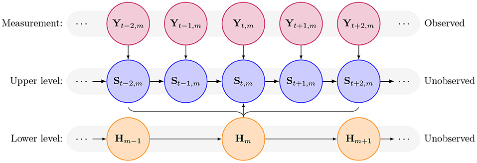
Figure 1. Diagram of dependence structure in the hierarchical hidden Markov model, showing the observed measurement layer, the high-resolution upper states, and the lower-resolution lower states, the latter two of which are unobserved latent states to be inferred.

The length of the sequence of the production states produced by the k-th internal state can be chosen according to the data collection process or dictated by the analysis. The corresponding K-state internal state process, ${\left\{H_m\right\}}_{m=1}^M$, is such that H_m serves as a proxy for a behavior occurring at a cruder time scale, namely throughout the m-th time frame (Leos Barajas and Michelot, 2018).

Assuming a Markov chain at the time frame level, then the m-th internal state is conditionally independent of all the others given the internal state at the (m − 1)-th time point, i.e., P(H_m|H_m−1, …, H₁) = P(H_m|H_m−1). Thus, the K × K t.p.m. for the internal states ${\left\{H_m\right\}}_{m=1}^M$ examines both the persistence in the internal states and the transitioning between them (Leos Barajas et al., 2017).

Defining the likelihood for the production states as in Equation (2), the conditional likelihood for a production state given the k-th internal state can be written as L_p(y_m|H_m = k), for k = 1, …, K. Denote by π^(I) a K-vector of initial probabilities for the internal states and by Γ^(I) the K × K t.p.m. for the internal state process. Then, the marginal likelihood for a hierarchically structured HMM can be expressed as

$\begin{array}{ll}{L}_{p,m}={\pi }^{(I)⊺}{P}^{(I)}(y_1){\displaystyle \prod _{m=2}^M}{\Gamma }^{(I)}{P}^{(I)}(y_m)1^T,& (3)\end{array}$

where $P^{(I)}(y_m)=diag(L_p(y_m|H_m=1),\dots ,L_p(y_m|H_m=K))$ is a K × K matrix (Leos Barajas et al., 2017).

2.3. Bayesian Inference

Markov chain Monte Carlo (MCMC) methods are simulation techniques that perform Monte Carlo integration using a Markov chain to generate observations from a target distribution. The Markov chain is constructed in such a way that, as the parameters are updated and the number of iterations t increases, the distribution associated with the t-th observation gets closer to the target distribution. Once the chain has converged to the stationary distribution π, the sequence of values taken by the chain can be used to obtain empirical (Monte Carlo) estimates of any posterior summary, including posterior distributions for parameters and latent variables. Therefore, MCMC algorithms are designed so that the Markov chain converges to the joint posterior distribution of the parameters given the model, the data, and prior distributions. Many different samplers have been created to construct Markov chains with the desired convergence properties and the efficiency of the resulting sample generation can vary drastically depending on the choice of algorithm and the tuning of parameters there-in.

The Gibbs sampler is an MCMC algorithm for generating random variables from a (marginal) distribution directly, without having to calculate the density. It is useful when the joint distribution of the parameters is not known explicitly or is difficult to sample from directly, but it is feasible to sample from the conditional distribution of each parameter. Given the state of the Markov chain at the t-th iteration, the Gibbs sampler successively draws randomly from the full posterior conditional distributions of θ_p.

The Metropolis-Hastings (henceforth MH) algorithm is a MCMC method for generating a sequence of states from a probability distribution from which it would be difficult to sample directly. The principle of the algorithm is to sample from a proposal (or candidate) distribution q, which is a crude approximation of the (posterior) target distribution h (Brooks et al., 2011). New parameter are subsequently drawn from the proposal distribution, often a symmetric distribution centered on the current parameter value, and hence exhibiting random walk (henceforth RW) behavior. Proposed parameter values are accepted with probability proportional to the ration of the posteriors, normalized by the ratio of the proposal densities. This induces a Markov process that asymptotically reaches the unique stationary distribution π(θ), such that π(θ) = h(θ|x).

2.4. Parallel Tempering

MH algorithms might get stuck in local maxima, especially in high-dimensional problems or multimodal densities. A feasible solution is trying to run a population of Markov chains in parallel, each with possibly different, but related stationary distributions. Information exchange between distinct chains enables the target chains to learn from past samples, improving the convergence to the target chain (Gupta et al., 2018).

Parallel tempering (PT) is a method that attempts periodic swaps between several Markov chains running in parallel at different temperatures, in order to accelerate sampling. Each chain is equipped with an invariant distribution connected to an auxiliary variable, the temperature β, which scales the “shallowness” of the energy landscape, and hence defines the probability of accepting an unsuitable move (Hansmann, 1997; Gupta et al., 2018). Following Metropolis et al. (1953), the energy of a parameter θ is defined as E[θ] = −logL[θ] − logp[θ], where L and p are the likelihood and the prior probability, respectively.

The algorithm is derived from the idea that an increase in the temperature smooths the energy landscape of the distribution, easing the MH traversal of the sample space. In fact, high temperature chains produce high density samples that accept unfavorable moves with a higher probability, thus exploring the sample space more broadly. As a result, switching to higher temperature chains allows the current sampling chain to circumvent local minima and to improve both convergence and sampling efficiency (Chib and Greenberg, 1995).

The Parallel Tempering algorithm for a parameter vector θ can be illustrated as follows:

• For s = 1, …, S swap attempts

1. For j = 1, …, J chains

I. For t = 1, …, T_MCMC iterations

i Propose a new parameter vector θ^*

ii Calculate the energy E[θ^*]

iii Set ${\theta }_{t+1}={\theta }^{*}$ with probability $min(1,e^{-{\beta }_j\Delta E_j})$, where $\Delta E_j=E_j\left[{\theta }^{*}\right]-E_j\left[{\theta }_{t-1}\right].$ Otherwise, set θ_t+1 = θ_t.

II. Record the value of the parameters and the energy on the final iteration

2. For each consecutive pair of chains (in decreasing order of temperature)

I. Accept swaps with probability min(1, e^−ΔβΔE), where ΔE = E_j − E_j−1 and Δβ = β_j − β_j−1.

The algorithm is similar to the standard Metropolis-Hastings algorithm, aside from the scaling of the acceptance ratio by the temperature parameter β_c and the additional swapping steps at regular intervals. If β_c = 1, then the exact posterior distribution of interest is being sampled; for values of β_c < 1, a higher temperature posterior is sampled, allowing acceptance of parameter moves further away from the current parameter value and facilitating moves outside of local modes. Ultimately, samples of the chain where β_c = 1 are retained and summary statistics calculated, with other chains used for improving convergence and subsequently discarded.

2.5. Data

The data relate to the harbor porpoise (Phocoena phocoena) dives presented in Leos Barajas et al. (2017). So as to build the hierarchical structure for the Hidden Markov Model, dive patterns were inferred at a crude scale K-state Markov process that identifies the general behavioral mode, and at a fine scale for state transitions at a dive-by-dive resolution, given the general behavior. Hence, a behavior occurring at a crude time scale can be connected to one of the K internal states, such that each internal state generates a distinct HMM, with the corresponding N production states generating the actual observation at a specific point in time (Leos Barajas et al., 2017). The production states are thus used to identify and categorize behavioral states, whilst internal states analyse patterns of changes in such behavioral states.

The crude time scale, hereafter also referred to as lower level, was built based on the notion that a dive pattern is typically adopted for several hours before switching to another one. For this purpose, observations recorded per second were grouped into hourly intervals, allowing each segment to be connected to one of the K = 2 HMMs with N = 3 (dive-by-dive upper level) states each.

Across the two dive-level HMMs, the same state-dependent distributions but different t.p.m.s were employed. This implied that any of the three types of dive (originating each from one of the three different production states) could occur in both lower level behavioral modes, but should not manifest equally often, on average, due to the different Markov chains active at the upper level. Moreover, supposing M time frames per individual, differences observed across y_m, for m = 1, …, M, were explained by considering the way in which a porpoise switches among the K internal states, while still modeling the transitions among production states at the time scale at which the data were collected (Leos Barajas et al., 2017).

The initial state distributions, for both the internal and the production state processes, were assumed to be the stationary distributions of the respective Markov chains.

The raw data was processed using the R package DIVEMOVE (Luque, 2007) and transformed into measures of dive duration, maximum depth, and dive wiggliness to characterize these Cetaceans' vertical movements at a dive-by-dive resolution, where dive wiggliness refers to the absolute vertical distance covered at the bottom of each dive (Leos Barajas et al., 2017). Such measures were considered to be the variables characterizing the model at the upper level, consisting of the observable fine-scale sequences y_m = (y_1,m, y_2,m, …, y_T,m) for m = 1, …, M.

Furthermore, in order to construct a relatively simple yet biologically informative model, gamma distributions, and contemporaneous conditional independence were assumed for the three variables. Hence, for any given dive, the observed variables were considered conditionally independent, given the production state active at the time of the dive (Leos Barajas et al., 2017).

2.6. Parameters

The parameters to be estimated through Bayesian inference are the ones defining the gamma distributions of the variables for all production states, with an additional point mass on zero for the dive wiggliness to account for null observations.

In principle, variables could be included both in the state-dependent processes, where they determine the parameters of the state-dependent distributions, and in the state processes, where they affect the transition probabilities (Langrock et al., 2012). However, in ecology the focus is usually on the latter, as the interest lies in modeling the effect of variables on state occupancy. Therefore, it is of interest to estimate also the transition probabilities matrices Γ (see section 2.1), and the corresponding initial distributions, for all the production states. The probabilities γ_ij at time t can be expressed as a function of some predictor η_ij(x_t) that in turn depends on a Q-dimensional vector containing the variables at time t x_t = (x_1,t, …, x_Q,t) (Langrock et al., 2012), where Q = 3.

In order to ensure identifiability when estimating the entries of Γ, the “natural” parameters γ_ij were transformed into “working” ones, η_ij (Leos Barajas et al., 2017). The γ_ij values were mapped by row onto the real line with the use of the multinomial logit link, to guarantee that 0 < γ_ij(x_t) < 1 and $\sum _{j=1}^N{\gamma }_{ij}(x_t)=1$ for ∀i, and the diagonal entries of the matrix were taken as the reference categories:

${\gamma }_{ij}=\frac{exp\left({\eta }_{ij}\right)}{{\displaystyle {\sum }_{k=1}^{N}exp\left({\eta }_{ij}\right)}},\text{ where }{\eta }_{ij}=\{\begin{array}{l}{\beta }_{ij}\text{\hspace{0.17em}\hspace{0.17em}\hspace{0.17em}\hspace{0.17em}\hspace{0.17em}\hspace{0.17em}if\hspace{0.17em}}i\ne j;\\ 0\text{ \hspace{0.17em}\hspace{0.17em}\hspace{0.17em}\hspace{0.17em}\hspace{0.17em}\hspace{0.17em}\hspace{0.17em}\hspace{0.17em}otherwise.}\end{array}$

For the sake of interpretability, the working parameters were eventually translated to their corresponding natural values.

Since HMMs lie within the class of mixture models, the lack of identifiability due to label switching i.e., a reordering of indices that can lead to same joint distribution, should be taken into account during the implementation of the algorithm and the interpretation of the corresponding results (Leos Barajas and Michelot, 2018).

As defined in section 2.1, the production state space is assumed to comprise N possible values, modeled as a categorical distribution. This implies that for each of the N possible states that a latent variable at time t can take, there is a transition probability from this state to each of the N states at time t + 1, for a total of N² transition probabilities. Since any one transition probability can be determined once the others are known, there are a total of N(N − 1) transition parameters to be identified (Zhongzhi, 2011). The same reasoning applies to the internal state space (see section 2.2), where for K possible states, once any one transition probability has been estimated, there are only K(K − 1) transition probabilities to determine.

Since each row of a t.p.m. has to add up to 1, the individual parameters of each row are connected and therefore there is fewer distinct parameters than there would appear. The first K − 1 elements were sampled independently of any constraint, whereas the last element of each set was estimated as the difference of 1 and the sum of the other estimates in the same set, according to section 2.6.

2.7. Prior Distributions

In ecological applications, prior distributions are a convenient means of incorporating expert opinion or information from previous or related studies that would otherwise be ignored (King et al., 2010). However, in the absence of any expert prior information, an uninformative prior Unif(0, 1) was specified for the proportion of observed zeros for the variable dive wiggliness. Constraining the means of the variables to be strictly positive, Log-Normal(log(100),1) distributions were taken as priors for their estimation, whereas Inv-Gamma(10⁻³, 10⁻³) were considered for their standard deviations.

Different prior distributions were specified for the transition matrix parameters. The first K − 1 or N − 1 entries of each row of the transition probability matrices were assumed to have a Beta(0.5, 0.5) prior, with the final element constrained by the sum of the other elements.

2.8. Implementation

The initial values for the estimation of parameters by the MH algorithm were obtained rounding to one decimal place the maximum log-likelihood estimates computed via direct numerical likelihood maximization (using the R function NLM, as in Leos Barajas et al., 2017). The transition probability matrices and the corresponding stationary distributions were kept fixed to their approximated values.

In this paper, proposal variances throughout the analyses were tuned adaptively to give an acceptance fraction between 25 and 40%, where the acceptance fraction is the simplest heuristic proxy statistic for tuning, defined as the ratio between the accepted proposed moves over the total number of iterations. Such range was considered throughout the implementation of all the different versions of the MH algorithm. The procedure was automated in order to perform an adjustment on the standard deviations δ of the RW every 100 iterations during burn-in and were then fixed for the RW updates of all the following iterations.

To further avoid correlations between parameters, two different approaches to block updating were devised for the MH algorithm. In the first case, the blocks were built bringing together the parameters of each variable across the three production states in order to update them simultaneously state-wise. For each variable, the means were updated first, followed by the corresponding standard deviations. Conversely, in the second scheme, parameters were still updated simultaneously state-wise, but the way blocks were arranged changed. The means for all the variables were updated first, and then the standard deviations were considered in the same order. In both cases, the proportions of null values observed for the variable maximum depth were studied separately, by simultaneous update.

For the parallel tempering algorithm, a Markov chain with a temperature value β = 1 was used to sample the true energy landscape, while three higher temperature chains with values of β equal to 0.75, 0.50, and 0.25 were employed to sample shallower landscapes. The acceptance probability was based on the difference in energy between consecutive iterations, scaled by the chain temperature, i.e., $min(1,e^{-{\beta }_c\Delta E_c})$, for c = 1, …, 4. Every T = 100 iterations a swap to the higher temperature chains was attempted, for a total of S = 160 swaps. Pilot tuning was performed on the first 6,000 iterations. The FOREACH and DOPARALLEL packages in R were used to parallelize such algorithm by allocating it to different cores (Weston and Calaway, 2019). As many clusters as the number of desired temperatures, and thus chains, were created and each allocated to a core, bearing in mind that it is recommended not to use all the available cores on the computer.

3. Results

3.1. Metropolis-Hastings and Variants

Employing the single-update MH algorithm, the fitted (dive-level) state-dependent distributions displayed in Figure 2 suggest three distinct dive types (see Figure 3 for the associated MCMC convergence diagnostics). Thresholds for the interpretation of variables in the three production states were identified as the 2nd and the 98th percentiles of the corresponding distribution.

1. Production state 1 captures the shortest (lasting <20.6 s), shallowest (between 1.2 and 7.9 m deep) and smoothest (<5.7 m absolute vertical distance covered) dives with small variance;

2. Production state 2 captures moderately long (7.6–77.5 s), moderately deep (4.1–28.5 m), and moderately wiggly (1–36.3 m) dives with moderate variance;

3. Production state 3 captures the longest (38–215.7 s), deepest (9.7–93.4 m), and wiggliest (8.2–120.7 m) dives with high variance.

FIGURE 2

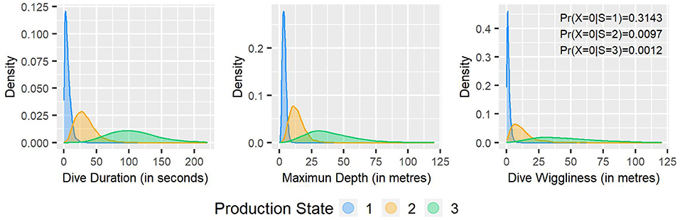
Figure 2. Fitted state-dependent distributions for dive duration, maximum depth, and dive wiggliness.

FIGURE 3

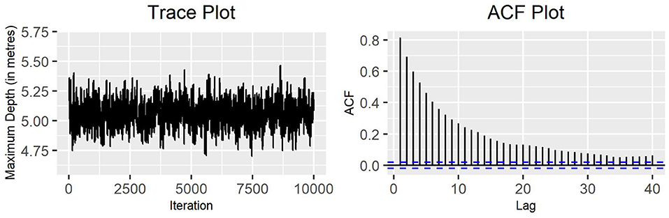
Figure 3. Single-update MH algorithm: trace plot and ACF plot of the standard deviation of the variable maximum depth for production state 2 (10,000 iterations).

From visual inspection of the trace plots of both the block-update MH algorithms, the first approach appeared to have slightly less autocorrelated chains with better mixing properties, allowing a broader traverse of the parameter space (see Figures 4, 5 for a specimen).

FIGURE 4

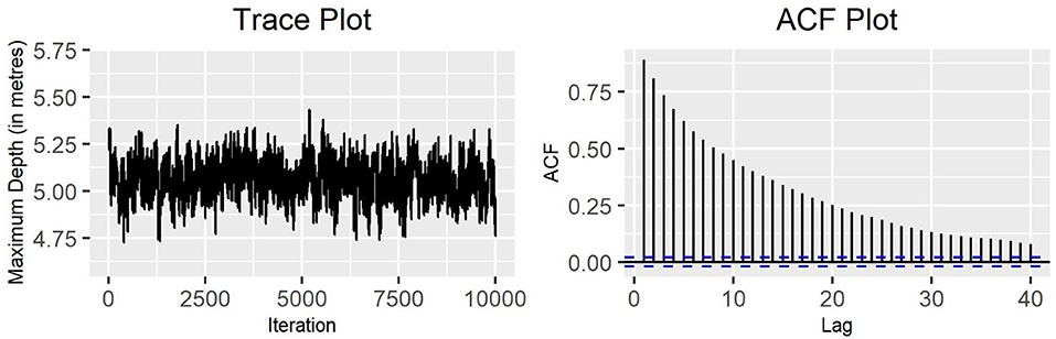
Figure 4. Block-update MH algorithm: trace plot and ACF plot of the standard deviation of the variable maximum depth for production state 2 (10,000 iterations) with blocks arranged by variable.

FIGURE 5

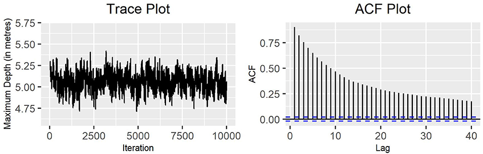
Figure 5. Block-update MH algorithm: trace plot and ACF plot of the standard deviation of the variable maximum depth for production state 2 (10,000 iterations) with blocks arranged by parameter.

The fact that a change in the autocorrelation values happened when altering the order of the blocks might suggest that it could have been worth it to reconsider the original single-update algorithm, varying the order in which parameters were updated. As a consequence, both algorithms were modified accordingly, relaxing the constraint of simultaneous update for the three production states. However, such strategy did not seem to perform much differently from the original MH algorithm nor from the respective block-wise update ones (see Supplementary Material for corresponding plots). In particular, multi-parameter algorithms performed slightly worse than the corresponding single-update versions. This could be due to the fact that, by updating multiple parameter at the same time during block-wise sampling, a move might have been rejected through being “poor” for some parameters, whilst it might have been “good” for the others (King et al., 2010).

It should also be noticed that for multiple parameter moves, the proposed changes are relatively small compared with the current values, as the proposal variance δ is smaller than for single-parameter updates, leading to a narrower exploration of the support of h (King et al., 2010).

3.2. Parallel Tempering

Looking at the trace plots and the ACF plots for the implemented MH algorithm, this strategy performs in a similar way to the single-update MH algorithm, with a good mixing in the chain and a slowly decreasing autocorrelation in the values. Figure 6 shows the behavior of the standard deviation of the variable maximum depth for production state 2, when performing parallel tempering with four temperature chains.

FIGURE 6

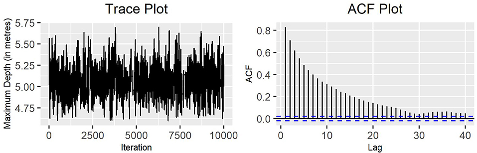
Figure 6. Trace plot and ACF plot of the standard deviation of the variable maximum depth for production state 2, obtained running four chains for parallel tempering on the MH algorithm (10,000 iterations).

Due to the high computational effort required by such an alternative, a different strategy was adopted to implement the MH algorithm with parallel tempering.

Considering again the standard deviation of the variable maximum depth for production state 2 (see Figure 7), it can be observed that employing a larger number of temperature chains for parallel tempering generates a better mixing and a roughly smaller autocorrelation between consecutive values.

FIGURE 7

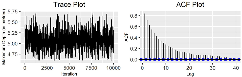
Figure 7. Trace plot and ACF plot of the standard deviation of the variable maximum depth for production state 2, obtained running seven chains for parallel tempering on the MH algorithm (10,000 iterations).

The main benefit of parallel tempering is its ability to explore multimodal distributions. This is can be seen in Figures 6, 7 as the range of parameter values visited by the algorithm is wider than any of the single MH algorithms. This suggests that there may be a multimodal nature to the parameter marginal distributions that the MH algorithm alone is not able to explore.

3.3. Prior Sensitivity Analysis

Prior sensitivity analysis was performed on the hyperparameters of the Beta distributions for the proportion of observed null values for the variable dive wiggliness. The MH algorithm with parallel tempering was rerun with Beta priors having both shape parameters either higher (α = β = 2) or lower (α = β = 0.5) than those specified in section 2.7. There was no evidence of significant changes in parameter estimates under varying priors, nor in the performance of the algorithm itself, as reflected in the almost unaffected acceptance rate of proposed moves.

3.4. Estimation of Transition Probabilities

In order to proceed with the estimation of the complete collection of parameters, one of the MH algorithms previously implemented was extended to estimate the transition probability matrices and the corresponding stationary distributions. The original single-update MH algorithm was selected, since it was the one that appeared to perform best. Figure 8 illustrates the behavior of the standard deviation of the variable maximum depth. It shows good mixing speed and the gradient of the autocorrelation function is not excessively shallow. A similar behavior can be observed for most of the other parameters (see Supplementary Material). It should be also mentioned that the acceptance fraction for the transition probabilities appeared to be quite high, ranging from nearly 36% to roughly 90% (see Supplementary Material).

FIGURE 8

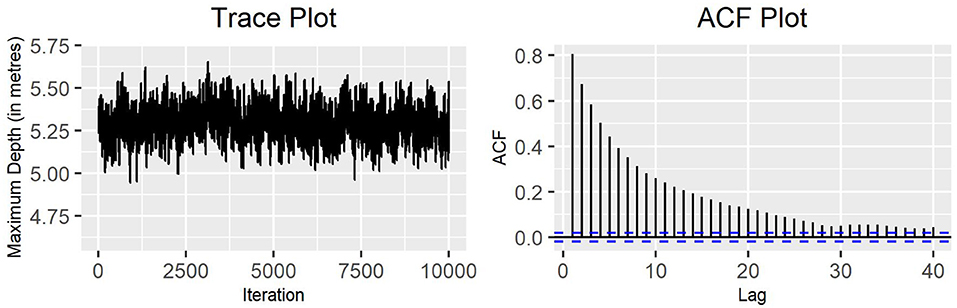
Figure 8. Single-update MH algorithm for the complete parameter set: trace plot and ACF plot of the standard deviation of the variable maximum depth for production state 2 (10,000 iterations).

4. Discussion

4.1. Interpretation of Results

According to the ACF plots for all the variables of the implemented MH algorithm, the means and the standard deviations present relatively high autocorrelation, even for larger values of l. In principle, such an issue was partially handled during the pilot tuning, by adjusting the standard deviation δ of the RW for the parameters of interest (see Table 1). However, pilot tuning alone proved itself inadequate to reduce the autocorrelation sufficiently. In order to improve the performance of the algorithm, different strategies were considered, such as block updates and parallel tempering.

TABLE 1

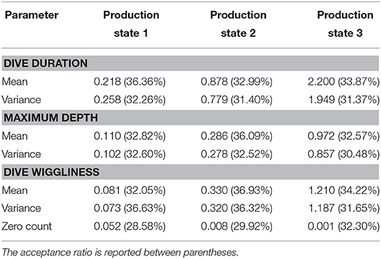
Table 1. Values obtained for the standard deviations δ of the Random Walk for each parameter after pilot tuning on 6,000 iterations.

Initially, the focus was on estimating the parameters of the gamma distributions of the variables for all production states, with an additional point mass on zero for the dive wiggliness to account for null observations.

For some parameters, the acceptance fraction fell outside the chosen thresholds, causing a fairly slow decrease in their autocorrelation functions and a non-optimal mixing speed for the corresponding chains. Thus, pilot tuning was conducted on the standard deviations of the random walk used for the proposal distributions, resulting in an overall improvement of the performance, yet insufficient to yield a significant reduction in the autocorrelation.

Conjecturing the presence of correlation between parameters, block-wise sampling was employed for simultaneous updates across the three production states. In the first case, the means for the three production states of all the variables were updated first, each followed by the corresponding standard deviations. In the second, all the means were updated first, followed by all the standard deviations, according to the same order in the variables. Although the first approach appeared to have less autocorrelated chains with better mixing properties than the second, the global performance turned out not to be better than the single-update one. In fact, the simultaneous update of multiple parameters might have caused the rejection of some moves through being inadequate for some parameters, whilst it might have been suitable for the others. Moreover, having a closer look at the trace plots and the ACF plots, a modest difference in their autocorrelation values was visible, hinting that the order in which parameters were updated might have had some influence on the performance.

Turek et al. (2016) considered block updating for MCMC algorithms to HMM and found improved performance compared to general algorithms within the NIMBLE software environment. However, the examples used were of a simpler nature to the one fitted here, which may explain why our results suggested careful adaptive tuning of proposals offered better results than block updating. In many cases it was necessary to make relatively small moves for the parameters to be accepted, leading to a narrower exploration of the support of the target distribution. For other parameters, instead, the acceptance rate turned out to be especially high. Indeed, the selection of non-ideal values for the standard deviations δ was mirrored in sub-optimal behavior of the chains, underlining a strong dependence on the choice of the proposal standard deviations. In fact, even if the chains exhibited good mixing speed, the autocorrelation values were still quite high even for large lags, especially for the production state 1. This suggested that an appropriate implementation of pilot tuning might have been instrumental in ameliorating the overall performance.

Therefore, a new MH algorithm involving parallel tempering was implemented. Different chains were run in parallel, each linked to an auxiliary temperature value that enabled to sample from a distinct energy landscape. At regular intervals, the behavior of the different chains was analyzed and a swap between temperature chains allowed, according to an acceptance probability that depended on the difference in both temperature and energy between different temperature chains. This facilitated the traverse of the sample space, exploiting the concept that higher temperature chains explore the sample space more broadly and are able to circumvent local minima. In the light of the fact that distributions on neighboring temperature levels need to have a considerable overlap, the number of temperatures was increased from four to seven. Running several chains from distinct points, as in parallel tempering, ensures the exploration of multimodal distributions. In fact, the posterior density plots for parallel tempering were globally unimodal, whereas for most of the other algorithms, many distributions showed some gentle spikes (see Supplementary Material). However, this strategy seemed to perform in a similar way to the single-update MH algorithm, with good mixing in the chain and a fairly high autocorrelation even for quite large lags. In particular, the performance of the MH algorithm with more temperature chains improved only to a limited extent with respect to the one with fewer chains. In practice, to have a reasonable acceptance rate, the temperatures need to be chosen carefully, and checked through preliminary runs. Moreover, the distributions on neighboring temperature levels need to have a considerable overlap (Hogg and Foreman-Mackey, 2018), suggesting that it would be appropriate to consider temperature values which are relatively close and possibly evenly spaced. For this purpose, the energy landscape was subsequently explored with a larger number C of chains, with temperatures β taking values equal to 1, 0.857, 0.714, 0.571, 0.429, 0.286, 0.143.

4.2. Comparison of Frequentist and Bayesian Results

The estimates found through Bayesian inference did not differ considerably from the ones obtained in Leos Barajas et al. (2017) using maximum likelihood estimation. This does not alter significantly the understanding of the ecological process, suggesting that the two methods might be equally effective in terms of interpreting the behavior of a harbor porpoise.

The first HMM might be indicative of a foraging behavior, particularly due to the extensive wiggliness characterizing the dives, which often indicates prey-chasing (van Beest et al., 2018). Conversely, the second HMM could represent a resting and/or a traveling behavior, due to the prevalence of relatively short, shallow and smooth dives.

Furthermore, it could be worthwhile to look at the estimates returned by the single-update MH algorithm, both when the t.p.m.s and their invariant distributions were kept constant (see Supplementary Material) and when instead they were included in the estimation process (see Table 2). Although one might expect the estimates for the first algorithm to be closer to the MLEs, as the hierarchical structure is more stable, the ones from the second algorithm are actually more similar to the frequentist results. In fact, while in the first case the transition probabilities and the stationary distributions are kept fixed to a very loose approximation of the classical estimates, in the second they will gradually converge to their actual estimates, easing the convergence of the whole set.

TABLE 2

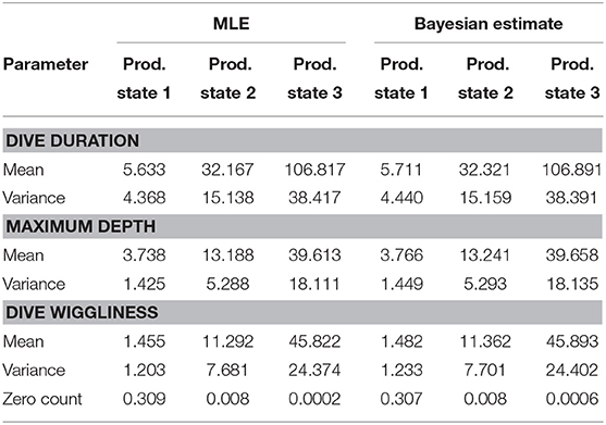
Table 2. Parameter estimates for the three production states, found through Maximum Likelihood Estimation and Bayesian Inference (on the complete collection of parameters).

The estimates of the single-update algorithm for the partial set of parameters could be also be compared to the ones obtained when employing parallel tempering (see Table 3). Even if they are roughly the same, the second algorithm is slightly closer to the values for the complete collection of parameters, using both classical and Bayesian inference. This is linked to the fact that employing parallel tempering enhances the sampler, by handling multimodality and conducting a wider exploration of the sample space.

TABLE 3

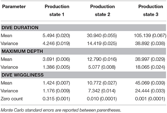
Table 3. Parameter estimates for the hyperparameters obtained through the MH algorithm with parallel tempering using seven chains.

5. Conclusions

The implemented algorithms appear to perform satisfactorily and to provide a sensible insight on behavioral modes connected to the analyzed movement data.

In such a way, a more robust structure might be constructed for block sampling, by specifying a suitable multi-dimensional proposal distribution, as recommended by King et al. (2010). Doing so, a more efficient strategy for pilot tuning could be devised as well. For instance, following the suggestions provided by Andrieu and Thoms (2008), the adjustment of the standard deviations δ of the RW updates could be performed automatically also for the transition probabilities. If possible, it would also be advisable to perform parallel tempering on the complete collection of parameters, or at least run multiple chains starting from overdispersed points in order to study the convergence of the chains.

Another important issue that may arise in the context of movement modeling is that the computational effort required to calculate the likelihood might be noticeably large compared to that of the simulation for the model of interest. In fact, for complex models, such as hierarchical HMMs—deriving an analytical formula for the likelihood function might be elusive or computationally expensive. Approximate Bayesian Computation methods are simulation-based techniques useful to infer parameters and choose between models, bypassing the evaluation of the likelihood function (Beaumont, 2010; Sunnåker et al., 2013). Following the results of Ruiz-Suarez et al. (2020), for this particular stochastic problem it could be worthwhile to employ a likelihood-free method based on the measure of similarity between simulated and actual observations. In fact, while the likelihood function is quite intractable due to the complicated relationship between parameters, simulating the movement of an harbor porpoise appears to be more straightforward. Therefore, through the simulation of dives from the HMM, relying on independent draws combined with data observed at regular time intervals, it would be possible to estimate the posterior distributions of model parameters (Sunnåker et al., 2013).

In animal movement modeling, estimation of the latent state sequence is not the primary focus, but rather a convenient byproduct of the HMM paradigm (Leos Barajas and Michelot, 2018). Estimated state-dependent distributions should be connected to biologically meaningful processes, though state estimation can help one visualize the results of the fitted models. The Viterbi algorithm (Viterbi, 1967) can be used for global state decoding, i.e., finding the sequence of the most likely internal and production states, respectively, given the observations.

Bayesian inference has proven to be a valid statistical instrument for modeling animal movement data according to a hierarchical HMM, providing an effective framework to infer drivers of variation in movement patterns, and thus describe distinct behaviors. Estimates of uncertainty in parameters and other summary statistics are also readily available as a direct outcome of the inference. The results highlight that parallel tempering, in particular, is beneficial in terms of building more realistic credible regions.

Although the computational times related to Bayesian inference tend to be larger than for the frequentist context, working in such a framework provides tools to circumvent issues common in statistical ecology and widens the opportunities for further analysis. For example, while there is no guarantee that a maximum likelihood procedure is really finding all the modes in a distribution, some Bayesian techniques enable the identification of multimodality, which is a frequent problem in mixture models and hidden Markov models. Indeed, different Bayesian algorithms return very similar point estimates, but some, such as a basic Metropolis Hastings sampler—fail to explore areas of the posterior space that are still consistent with the data, hinting to multimodality. The tuned MH algorithm will tend to focus in on local modes to optimize acceptance rates, rather than learning about additional modes away from the current area of high probability. Conversely, parallel tempering allows the sampling of the full parameter space more readily, improving the overall estimation of uncertainty and credible regions. Another prerogative of the Bayesian framework is incorporating in the MCMC algorithm biological a priori knowledge, which might provide a considerable benefit in terms of the estimation, particularly in data sparse examples. HMMs can be used to model many other types of ecological data, including mark-recapture data (Turek et al., 2016), and similar approaches could also be developed for these models.

Keeping in mind that different algorithms and computational methods are usually complementary—not competitive, the tools available to the Bayesian paradigm provide a powerful and flexible framework for the analysis of complex high-dimensional stochastic processes.

Data Availability Statement

Publicly available datasets were analyzed in this study. This data can be found at: https://static-content.springer.com/esm/art%3A10.1007%2Fs13253-017-0282-9/MediaObjects/13253_2017_282_MOESM1_ESM.rdata.

Author Contributions

BS was responsible for initiating the idea for the paper, while GS conducted the majority of the analyses and wrote the code under BS's supervision. The manuscript content was written by GS with considerable editing and contributions from BS.

Conflict of Interest

The authors declare that the research was conducted in the absence of any commercial or financial relationships that could be construed as a potential conflict of interest.

Supplementary Material

The Supplementary Material for this article can be found online at: https://www.frontiersin.org/articles/10.3389/fevo.2021.623731/full#supplementary-material

Supplementary figures and parameter estimates can be found in the Supplementary Material. Code for running the analyses is available at https://github.com/giada-sacchi/Towards-efficient-Bayesian-approaches-to-inference-in-HHMM-for-animal-behaviour.

References

Adam, T., Griffiths, C. A., Leos-Barajas, V., Meese, E. N., Lowe, C. G., Blackwell, P. G., et al. (2019). Joint modelling of multi-scale animal movement data using hierarchical Hidden Markov Models. Methods Ecol. Evol. 10, 1536–1550. doi: 10.1111/2041-210X.13241

CrossRef Full Text | Google Scholar

Andrieu, C., and Thoms, J. (2008). A tutorial on adaptive MCMC. Stat. Comput. 18, 343–373. doi: 10.1007/s11222-008-9110-y

CrossRef Full Text | Google Scholar

Beaumont, M. (2010). Approximate bayesian computation in evolution and ecology. Annu. Rev. Ecol. Evol. Syst. 41, 379–406. doi: 10.1146/annurev-ecolsys-102209-144621

CrossRef Full Text | Google Scholar

Brooks, S., Gelman, A., Jones, G., and Meng, X. (2011). Handbook of Markov Chain Monte Carlo. Boca Raton, FL.

Google Scholar

Chib, S., and Greenberg, E. (1995). Understanding the metropolis-hastings algorithm. Am. Stat. 49, 327–335. doi: 10.1080/00031305.1995.10476177

CrossRef Full Text | Google Scholar

Fine, S., Singer, Y., and Tishby, N. (1998). The hierarchical Hidden Markov Model: analysis and applications. Mach. Learn. 32, 41–62. doi: 10.1023/A:1007469218079

PubMed Abstract | CrossRef Full Text | Google Scholar

Gupta, S., Hainsworth, L., Hogg, J. S., Lee, R. E. C., and Faeder, J. R. (2018). “Evaluation of parallel tempering to accelerate bayesian parameter estimation in systems biology,” in 26th Euromicro International Conference on Parallel, Distributed and Network-Based Processing (Cambridge). doi: 10.1109/PDP2018.2018.00114

PubMed Abstract | CrossRef Full Text | Google Scholar

Hansmann, U. H. (1997). Parallel tempering algorithm for conformational studies of biological molecules. Chem. Phys. Lett. 281, 140–150. doi: 10.1016/S0009-2614(97)01198-6

CrossRef Full Text | Google Scholar

Hogg, D. W., and Foreman-Mackey, D. (2018). Data analysis recipes: using Markov Chain Monte Carlo. Astrophys. J. Suppl. 236:11. doi: 10.3847/1538-4365/aab76e

CrossRef Full Text | Google Scholar

Joo, R., Bertrand, S., Tam, J., and Fablet, R. (2013). Hidden Markov Models: the best models for forager movements? PLoS ONE 8:e71246. doi: 10.1371/journal.pone.0071246

PubMed Abstract | CrossRef Full Text | Google Scholar

King, R., Morgan, B. J. T., Gimenez, O., and Brooks, S. P. (2010). Bayesian Analysis for Population Ecology. Boca Raton, FL: Chapman & Hall/CRC.

Google Scholar

Langrock, R., King, R., Matthiopoulos, J., Thomas, L., Fortin, D., and Morales, J. M. (2012). Flexible and practical modeling of animal telemetry data: Hidden Markov Models and extensions. Ecology 93, 2336–2342. doi: 10.1890/11-2241.1

PubMed Abstract | CrossRef Full Text | Google Scholar

Leos Barajas, V., Gangloff, E., Adam, T., Langrock, R., van Beest, F., Nabe-Nielsen, J., et al. (2017). Multi-scale modeling of animal movement and general behavior data using Hidden Markov Models with hierarchical structures. J. Agric. Biol. Environ. Stat. 22, 232–248. doi: 10.1007/s13253-017-0282-9

CrossRef Full Text | Google Scholar

Leos Barajas, V., and Michelot, T. (2018). An introduction to animal movement modeling with Hidden Markov Models using Stan for bayesian inference. arXiv 1806.10639.

Luque, S. (2007). Diving behaviour analysis in R. R News 7, 8–14. Available online at: https://www.r-project.org/doc/Rnews/Rnews_2007-3.pdf (accessed August 20, 2020).

Google Scholar

McClintock, B. T., Langrock, R., Gimenez, O., Cam, E., Borchers, D. L., Glennie, R., et al. (2020). Uncovering ecological state dynamics with Hidden Markov Models. Ecol. Lett. 23, 1878–1903. doi: 10.1111/ele.13610

PubMed Abstract | CrossRef Full Text | Google Scholar

Metropolis, N., Rosenbluth, A. W., Rosenbluth, M. N., Teller, A. H., and Teller, E. (1953). Equation of state calculations by fast computing machines. J. Chem. Phys. 21, 1087–1092. doi: 10.1063/1.1699114

CrossRef Full Text | Google Scholar

Patin, R., Etienne, M. P., Lebarbier, E., Chamaillé-Jammes, S., and Benhamou, S. (2020). Identifying stationary phases in multivariate time series for highlighting behavioural modes and home range settlements. J. Anim. Ecol. 89, 44–56. doi: 10.1111/1365-2656.13105

PubMed Abstract | CrossRef Full Text | Google Scholar

Ruiz-Suarez, S., Leos-Barajas, V., Alvarez-Castro, I., and Morales, J. M. (2020). Using approximate bayesian inference for a “steps and turns” continuous-time random walk observed at regular time intervals. PeerJ 8:e8452. doi: 10.7717/peerj.8452

PubMed Abstract | CrossRef Full Text | Google Scholar

Schliehe-Diecks, S., Keppeler, P., and Langrock, R. (2012). On the application of mixed Hidden Markov Models to multiple behavioural time series. Interface Focus 2, 180–189. doi: 10.1098/rsfs.2011.0077

PubMed Abstract | CrossRef Full Text | Google Scholar

Sunnåker, M., Busetto, A. G., Numminen, E., Corander, J., Foll, M., and Dessimoz, C. (2013). Approximate bayesian computation. PLoS Comput. Biol. 9:e1002803. doi: 10.1371/journal.pcbi.1002803

CrossRef Full Text | Google Scholar

Touloupou, P., Finkenstädt, B., and Spencer, S. E. F. (2020). Scalable bayesian inference for coupled Hidden Markov and Semi-Markov Models. J. Comput. Graph. Stat. 29, 238–249. doi: 10.1080/10618600.2019.1654880

PubMed Abstract | CrossRef Full Text | Google Scholar

Tucker, B. C., and Anand, M. (2005). On the use of stationary versus Hidden Markov Models to detect simple versus complex ecological dynamics. Ecol. Modell. 185, 177–193. doi: 10.1016/j.ecolmodel.2004.11.021

CrossRef Full Text | Google Scholar

Turek, D., de Valpine, P., and Paciorek, C. J. (2016). Efficient Markov Chain Monte Carlo sampling for Hierarchical Hidden Markov Models. Environ. Ecol. Stat. 23, 549–564. doi: 10.1007/s10651-016-0353-z

CrossRef Full Text | Google Scholar

van Beest, F. M., Teilmann, J., Dietz, R., Galatius, A., Mikkelsen, L., Stalder, D., et al. (2018). Environmental drivers of harbour porpoise fine-scale movements. Mar. Biol. 165:95. doi: 10.1007/s00227-018-3346-7

PubMed Abstract | CrossRef Full Text

Viterbi, A. (1967). Error bounds for convolutional codes and an asymptotically optimum decoding algorithm. IEEE Trans. Inform. Theory 13, 260–269. doi: 10.1109/TIT.1967.1054010

CrossRef Full Text | Google Scholar

Weston, S., and Calaway, R. (2019). Getting Started With doParallel and Foreach. Vignette, CRAN. Available online at: http://users.iems.northwestern.edu/~nelsonb/Masterclass/gettingstartedParallel.pdf

Google Scholar

Yoon, B. J. (2009). Hidden Markov Models and their applications in biological sequence analysis. Curr. Genomics 10, 402–415. doi: 10.2174/138920209789177575

PubMed Abstract | CrossRef Full Text | Google Scholar

Zhongzhi, S. (2011). Advanced Artificial Intelligence. Signapore: World Scientific Pub. Co. Inc.

Zucchini, W., MacDonald, I. L., and Langrock, R. (2016). Hidden Markov Models for Time Series: An Introduction Using R. Boca Raton, FL: Chapman & Hall/CRC.

Google Scholar